rspa.royalsocietypublishing.org
Research
Article submitted to journal
Subject Areas:
Nonlinear mechanics, Astrophysics
Keywords:
Foucault pendulum, Berry geometric phases, pendulum tilt, syzygies, two-form, gyroscopic effects
Author for correspondence:
R. Verreault
e-mail: [email protected]
Gyroscopic theory of the Foucault pendulum:
New Berry phases and sensitivity to syzygies
R. Verreault 1
1 Department of Fundamental Sciences, University of Quebec at Chicoutimi, Saguenay (Quebec) Canada 0000-0003-4638-1892
The normal way of exploiting a Foucault pendulum is by considering the total precession angle described during a complete cycle and to cumulate those elementary precession increments in order to yield a macroscopic precession angle. Said precession angle has been shown by Hanney to constitute a geometric phase in the sense described by Berry in 1984. The above precession increments per cycle have also been described by Berry as the result of a mathematical two-form corresponding to a pair of orthogonal pendulum circular oscillation states. In this article, the pendulum is analyzed on a half-cycle basis, as a pair of contra-rotating gyroscopes spinning about a horizontal axis. During two consecutive half-cycles, these two gyroscopes, acting in sequence, describe equal precession angles about the vertical axis, but in opposite directions, when the horizontal axis is forced by gravity to change its orientation in free space as the Earth is revolving. That gives rise, within each complete cycle, to a novel 8-shaped orbit. The cumulative precession angle difference over many complete cycles constitutes a new geometric phase of the Berry type. It can be described by a new two-form corresponding to the spin states of the two contra- rotating gyroscopes. Instead of evaluating the effect of the two-form after each complete oscillation cycle, the new two-form is assessed after each half cycle and the difference between the half-cycle effects is cumulated.
The new geometric phase is related to the tilt rate of the local vertical in free space. Thanks to an 18-hour- duration pendulum experiment, evidence of the novel 8-shaped orbit is given. The Foucault pendulum is no longer considered in its geocentric environment, but in the barycentre frame of different celestial bodies.
Sensitivity to syzygies between pendulum and said celestial bodies is discussed.
c The Authors. Published by the Royal Society under the terms of the Creative Commons Attribution License http://creativecommons.org/licenses/
by/4.0/, which permits unrestricted use, provided the original author and source are credited.
2
rspa.ro y alsocietypub lishing.org Proc R Soc A 0000000 .. .. .. .. .. .. .. .. .. .. .. .. .. .. .. .. .. .. .. .. .. .. .. .. .. .. .. .. ..
1. Introduction
Several experimenters have reported all sorts of perturbations affecting Foucault pendulum behavior [1,2]. On the other hand, since the early days of the Foucault pendulum, many theoreticians have also tried to describe that highly nonlinear system using the pendulum Hamiltonian and perturbation theory. In particular, the following four milestones in Foucault pendulum evolution are worth mentioning.
• As soon as 1840, G.B. Airy [3] addressed the problem of elliptic orbits for the spinning balls of speed governors of steam engines, which are equivalent to a spherical pendulum oscillating almost in a circular mode (the so-called Bravais pendulum). His conclusion was that such a circular mode is unstable and evolves into an almost circular elliptic mode where the major axis undergoes a precession at the rate 3ωαβ/8; (α and β are the major-axis and minor-axis angular amplitudes, respectively). Eleven years later, Airy [4]
obtained a similar result for a Foucault pendulum when the bob trajectory is a narrow ellipse.
• In 1879, in his doctoral thesis under the incitation of Gustav Kirchhoff, Heike Kamerlingh Onnes [5] applied perturbation methods used for celestial mechanics to the Hamiltonian of the Foucault pendulum in the 2-dimensional (2D) linear oscillator approximation. He could demonstrate the onset of elliptical bob orbits due to anisotropy of the crossed- knives suspension of his pendulum.
• From 1954 to 1960, thanks to a series of 7 one-month-duration experiments involving 3 pendulum launches per hour, the French physicist Maurice Allais [6, 7] established significant correlations between the position of the Moon and systematic azimuth fluctuations of the anisotropy axes of his paraconical pendulum (the so-called periodic or general Allais effect). Up to now, no conventional theory has provided a quantitative explanation of that effect.
• More recently in 2013, Maya et al. [8], using perturbation theory, generalized the Airy effect for the ideal spherical pendulum (ISP) with arbitrary ellipse axis ratios β/α and included a spin-orbit coupling precession contribution to Airy precession for the physical spherical pendulum (PSP). So, the experimental spin-orbit coupling data observed by Allais in 1955 [9], but not described as such by himself, have been explained for the first time. In fact, the onset of clockwise (cw) Foucault precession right from the start is accompanied by an opposite, counter-clockwise (ccw) spin of the bob in order to maintain the initial zero angular momentum about the vertical in the rotating laboratory frame.
When an elliptical orbit develops somewhat later due to suspension anisotropy, part of the spin momentum is converted into a precession contribution that adds up to the ISP Airy precession. Those authors have proposed the name Allais precession for that Airy-like precession of the PSP.
In 1984, Michael Berry [10,11] has shown via parallel transport of vectors along a curved hypersurface that the state of a relativistic particle with spin is described not only by the dynamic phase of the cyclic motion, but also by a geometric phase that is totally independent of the spin degree of freedom, depending only on the curved path described by the particle along a geodesic. One year later, John Hannay [12] extended that theory to the case of periodic classical systems described by action-angle variables, such as the Foucault pendulum, where a virtual two-form made of two non-degenerate orthogonal circular oscillation states is shown to generate a cumulative Berry phase in the form of precession of the oscillation azimuth of the resultant rectilinear oscillation. In this paper, a new kind of two-form made of the spin states of two contra-rotating gyroscopes is shown to generate a new set of differential Berry phases.
It has been customary to speak of the spin of a pendulum as the rotation of the bob about
its axis of symmetry passing through the suspension point. Spin-orbit coupling arises from the
invariance of the total vertical component of angular momentum [6,13]. However, the ISP made
3
rspa.ro y alsocietypub lishing.org Proc R Soc A 0000000 .. .. .. .. .. .. .. .. .. .. .. .. .. .. .. .. .. .. .. .. .. .. .. .. .. .. .. .. ..
up of a point mass revolving about a suspension point via a massless inextensible wire has no spin degree of freedom in the sense just described. Nevertheless, its general elliptic orbit can be thought of as the superposition of a circular orbit with angular amplitude β and a rectilinear orbit with angular amplitude (α − β). This latter component can be represented by two contra-rotating spinning gyroscopes.
In the following, two measuring systems of pendulum motion (or alidades) that are appropriate for the proposed motion analysis are described. Then a numerical integration of the gyroscopic differential equation is performed within a half-cycle of oscillation, instead of being averaged over a complete cycle as it is often the case in perturbation theory. Finally, the feasibility of the method for detecting and/or measuring anomalies caused by the motion of neighboring celestial bodies is discussed.
2. Materials and Methods
(a) The alidades
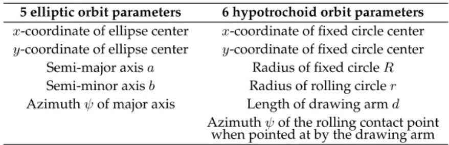
A word must be said about typical experimental setups suitable for demonstrating the phenomena of interest. It is customary to represent the general trajectory of the Foucault pendulum bob over one oscillation cycle by its projection on a horizontal plane in the form of an ellipse whereas five parameters are necessary for its complete determination. However, at the level of precision needed for the forthcoming analysis, that ellipse must be replaced by a more exact and more general mathematical curve, namely the hypotrochoid. The parameters to be determined in each case are listed in Table 1. More details are shown in Appendix A.
Table 1.
Parameters needed to characterize the elliptic and hypotrochoid orbits of the bob.
5 elliptic orbit parameters 6 hypotrochoid orbit parameters x-coordinate of ellipse center x-coordinate of fixed circle center y-coordinate of ellipse center y-coordinate of fixed circle center
Semi-major axis a Radius of fixed circle R Semi-minor axis b Radius of rolling circle r Azimuth ψ of major axis Length of drawing arm d
Azimuth ψ of the rolling contact point when pointed at by the drawing arm
In the experiments conducted by the author between 2001 and 2010, video imaging of optically
observable alidades has been used. A set of retro-reflecting markers (2 mm dia.) was attached to
the pendulum bob and to the surrounding alidade fixed to the floor [14], in accordance with a
remote sensing technology developed in the 1980’s [15,16]. An interesting feature of recording
bob motion in that way is the creation of a large amount of redundancy which can be taken
advantage of for reducing experimental uncertainties. As an example, the barycenter of the light
intensity distribution of a marker image in Reference [14] could be determined to ±0.1 pixel in
each dimension. With a 1.8-mm size pixel on the floor alidade and a 17.4-m long pendulum,
that means a precision of angular determination of 10
−5rad in each video image. In such an
experiment, one half-orbit is composed of 126 video images from which 6 parameters must be
determined. There remains 120 degrees of freedom for reducing statistical uncertainty. So, the
instantaneous tilt angle of the pendulum line when passing near the bottom rest point (i.e. the
angular semi-minor axis β if the orbit was an ellipse) can be determined with a precision of the
order of 10
−6rad (18 µm on the floor). If one is dealing with slowly varying tilt over a time scale
of say 10 hours, a 3-hour running average comprising ~2500 half-cycles leaves a tilt statistical
measuring error of 2 · 10
−8rad .
4
rspa.ro y alsocietypub lishing.org Proc R Soc A 0000000 .. .. .. .. .. .. .. .. .. .. .. .. .. .. .. .. .. .. .. .. .. .. .. .. .. .. .. .. ..
Another type of alidade that also has the potential of detecting tilt angle is based on a pattern of light beams disposed at various azimuths and centered on the pendulum rest point. Timings of disappearance and reappearance of the consecutive light beams at sub-microsecond resolution are combined to yield precession angle for each half cycle. Further experimentation is still necessary with that system in order to enable an assessment of its ultimate precision. However, preliminary experimentation with that alidade shows that the precision should be comparable with that of video imagery.
(b) Gyroscopic effects
The idea of considering the gyroscopic effects of the swinging motion is not necessary new [17].
However, to the author’s knowledge, no quantitative results are given and the alleged effects are sometimes highly hypothetical. It could be argued that many quantitative treatments using perturbation methods with action-angle variables [18] or Euler angles [8] do implicitly include the gyroscopic effects. It must be pointed out, though, that those methods generally imply parameter averaging over one complete cycle, contrary to the approach put forward in the present article.
In fact, over one complete cycle, the alleged gyroscopic effects cancel out and turn out to be unmeasurable.
The essential feature of the method consists of considering the back and forth motion within a rectilinear oscillation as equivalent to a pair of opposite gyroscopes acting in sequences of one half-cycle duration each. Hannay [12] does include an action-angle treatment of the Foucault pendulum where the tilting pendulum axis describes a conical surface about the earth axis. But that construction is only used to define the so-called Hannay angle (the solid angle of the cone) which merely equals the total precession (or direct precession) angle of the pendulum after one cycle of Earth rotation.
During an infinitesimal time interval dt, a pendulum swinging in a vertical plane about a horizontal axis can be seen as a gyroscope for that time interval. Since the horizontal gyroscope axis (spin axis) is forced to remain horizontal through the action of Earth gravity on the bob, the vertical oscillation plane undergoes precession in a given sense during the first half-cycle. For the second half-cycle, the gravitational torque on the spin axis remains the same but the reversed angular momentum of the reversed gyroscope causes a precession in the same amount, but opposite sense, to take place, thus cancelling the effect of the first half-cycle. Instead of evaluating, as usual, the effect of the gyroscopic two-form after each complete oscillation cycle, that new two- form is assessed after each half-cycle and the difference between the half-cycle precession angles is cumulated in the form of a geometric phase. This new geometric phase is in fact related to the total tilt angle of the pendulum’s vertical in free space after time t. The traditional Foucault effect, which is based on the two-form consisting of the two non-degenerate rotation velocity components about the vertical for the two orthogonal circular oscillations in the laboratory frame, is maximal at the poles and null at the equator. On the contrary, the new two-form effect sensitive to tilt rate is null at the poles and maximal at the equator. This new effect conveys information that is not available in the traditional Foucault effect. For any given latitude, the sum of the half-cycle precession angles describes the local rotation velocity of the horizontal surface about the vertical, while their difference describes the tilt rate of the vertical as the pendulum travels through space.
(c) Free space environment
The traditional Foucault pendulum has been quantitatively analyzed in a geocentric environment
where any possible tidal perturbation, introduced in the form of external forces or accelerations
originating from the Moon and the Sun [12,19], was evaluated in terms of possible changes that
it could cause in precession rate and in ovalization rate (rate of growth of minor axis). Tilt rate
is merely brushed aside [20] since, from experiment, the tilt rate of the vertical at the equator
generates no net precession. As a matter of fact, in a geocentric frame, a tilt of the vertical refers
to the angle subtended by the ellipsoid center and the center of curvature of a gravitational
5
rspa.ro y alsocietypub lishing.org Proc R Soc A 0000000 .. .. .. .. .. .. .. .. .. .. .. .. .. .. .. .. .. .. .. .. .. .. .. .. .. .. .. .. ..
equipotential referred to the pendulum site. However, for a pendulum at a given site, that tilt angle is constant. So, there is no tilt rate in a geocentric frame.
The new attempt to address pendulum anomalies in this article takes the Earth translation through space into account. The accelerations and decelerations of a Foucault pendulum in free space along its geodesic must translate into changes in tilt angle that can be detected to first order only by the new two-form.
Since there are several different time scales involved, typical calculations of Moon effects over a time scale of a few days can be performed by analyzing the influence of the Moon in an inertial frame attached to the Earth-Moon barycenter. In that frame, the pendulum suspension point S describes a sort of complicated helico-hypotrochoid in free space. One may have a rough idea of that orbit shape by imagining a torus supporting a sort of skewed slinky that comes back into a path close to the preceding one after 27.32 days. That defines a geodesic along which the accelerations and decelerations applied to a spherical pendulum are analyzed in terms of varying tilt rate, whence the need for an approach sensitive to tilt rate like the one described in this article.
It has been argued by Allais [19] that a calculation based on tidal acceleration differences at the scale of a pendulum swing that could induce a precession torque about the vertical axis yields, in the laboratory frame, values 10
8times smaller than those of some observed anomalies. Applying Pippard’s [26] perturbation formalism to that problem leads to the same conclusions. On the other hand, it was also considered by Allais that tilt angle has no effect on precession torque, since a constant lateral acceleration does not affect precession rate. The author agrees with that opinion about tilt angle. However, that statement completely ignores the gyroscopic effects that are in fact proportional to tilt rate instead of tilt angle. For studying gyroscopic effects and the property of fixity in space of the spin axis, it is necessary to revert from the laboratory frame toward an inertial frame in free space. Once the results about orbit shape are obtained, it then becomes pertinent to look back at that orbit in the laboratory frame, where pendulum motion measurements are normally made.
3. Quantitative results
(a) The spherical pendulum in an inertial frame
Let us first consider the ISP (point mass) in an inertial reference frame SX
0Y
0Z
0, hence without Foucault effect and without any spin degree of freedom of the extensionless bob about the pendulum line. One of the known solutions of the equations of motion is the elliptical orbit of figure [1]. According to standard textbooks [21], during the time interval dt, pendulum motion about the suspension point S can be described through Euler angles θ, ϕ, ψ, as shown in Appendix B. Of course, in usual pendulum operation, the nodes will never be reached by the bob, but if the examined motion during the time interval dt would go on without recall torque, the bob would go up to the ascending node and come back down from the descending node, and so on. During the time increment dt under study, bob motion along the orbit is a tiny arc of an instantaneous revolution (spin angle) about the suspension point in the XY -plane with angular velocity ϕ ˙ generating the instantaneous angular momentum vector L along the SZ-axis. The inertial horizontal axes X
0Y
0at the suspension point are reported onto the laboratory floor to show the horizontal projection of the bob orbit. The angle ψ measures the precession of the line of nodes as time elapses. Note that ON is parallel to the incremental orbit arc at all times. Gravity along the vertical OZ
0-axis generates a torque ~ τ =
dLdtwhere dL lies in a horizontal plane and is perpendicular to the vertical plane containing the angle γ, in such a way that
sin
2γ = sin
2(π/2 − θ) + sin
2ϕhttps : //f r.overleaf.com/project/ (3.1)
The momentum increment dL, which is always horizontal, is not in general perpendicular
to the spin axis SZ, so that, unlike the spinning-top approximation, |L| is not constant. The
successive vectors dL generate the elliptic hodograph of L as shown. The height L
Z0of the
hodograph above (or below, for cw orbits) the suspension point is the constant vertical angular
6
rspa.ro y alsocietypub lishing.org Proc R Soc A 0000000 .. .. .. .. .. .. .. .. .. .. .. .. .. .. .. .. .. .. .. .. .. .. .. .. .. .. .. .. ..
momentum component identified as the orbital angular momentum. It becomes zero for a rectilinear bob oscillation in a vertical plane. In this situation, L simply oscillates in magnitude along a perpendicular to the oscillation plane through S.
Figure 1.
Geometry of the spinning pendulum in the inertial frame SX
0Y
0Z
0(non-rotating Earth) during the time
interval dt . Euler angles θ, ϕ, ψ are the same as those of the spinning top. During that time increment, bob motion
along the orbit is part of an instantaneous revolution (spin) about the suspension point in the XY -plane (in red) with
angular velocity ϕ ˙ generating the instantaneous angular momentum vector dL (in red) along the spin axis SZ . The
inertial horizontal axes X
0Y
0at the suspension point are reported onto the laboratory floor alidade to show the horizontal
projection of the bob orbit. The line of nodes ON (not shown at the suspension point for clarity) is the intersection line of
the horizontal plane with the XY -plane attached to the spinning pendulum. The angle ψ measures the precession of that
XY -plane with respect to the OX -axis. Gravity along the vertical OZ
0-axis generates a torque ~ τ = dL/dt where dL
lies in a horizontal plane and is perpendicular to the vertical plane containing the angle γ . Note that dL has a component
along SZ so that, unlike in the spinning-top approximation, |L| is not constant. The successive vectors dL generate the
elliptic hodograph of L . Therefore, the projected orbit ellipse and the ellipse of the hodograph of L are both horizontal
ellipses with the same ellipticity but with orthogonal major axes. The height L
Z0of the hodograph above (or below, for cw
orbits) the suspension point is the constant orbital angular momentum. It becomes zero for a rectilinear bob oscillation in
the projection plane, say along OX
0. In that situation, L simply oscillates in magnitude along the SY
0-axis. The elliptical
orbit is due to a two-fold action of gravity: (a) gravity generates a recall torque along OZ for the swing angle ϕ in the
XY -plane; (b) its tendency (horizontal torque component normal to OZ ) to bring the OZ -axis toward a horizontal plane
generates a precession of the XY -plane about the vertical, hence the well-known elliptic orbit of the bob which, in fact,
is the result of gyroscopic precession of the XY -plane over one oscillation cycle.
7
rspa.ro y alsocietypub lishing.org Proc R Soc A 0000000 .. .. .. .. .. .. .. .. .. .. .. .. .. .. .. .. .. .. .. .. .. .. .. .. .. .. .. .. ..
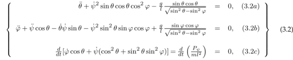
From the Lagrangian of the spherical pendulum in Appendix B, the respective equations of motion for the generalized coordinates θ, ϕ and ψ are
θ ¨ + ˙ ψ
2sin θ cos θ cos
2ϕ −
gl√
sinθcosθsin2θ−sin2ϕ
= 0, (3.2a)
¨
ϕ + ¨ ψ cos θ − θ ˙ ψ ˙ sin θ − ψ ˙
2sin
2θ sin ϕ cosϕ +
gl√
sinϕcosϕsin2θ−sin2ϕ
= 0, (3.2b)
d
dt
[ ˙ ϕ cos θ + ˙ ψ(cos
2θ + sin
2θ sin
2ϕ)] =
dtd Pψ
ml2
= 0, (3.2c)
(3.2)
It follows from the last equation that the angular momentum conjugated to the precession angle is a constant of the motion. Its magnitude corresponds to the height of the momentum hodograph above (or below) the suspension point S, in Figure [1]. However, unlike the spinning- top approximation, the spin angular momentum of the pendulum is not a constant of the motion.
It is subject to acceleration due to a gravitational recall torque.
Figure 2.
Projection of the orbit on the horizontal alidade showing the pedal curve described by the orthogonal projection P of the ellipse center onto a XY -plane tangent to the ellipse at the instantaneous bob position B . The XY -plane subtends the tilt angle ϑ at the suspension point. P acts as the instantaneous origin for ϕ in the XY -plane. With four passages at zero over one pendulum cycle, ϕ shows a strong second harmonic component, except for the circular orbit ( ϕ = 0 ) and for the rectilinear orbit [ ϕ = α cos (ωt − ϕ
0) ].
In the usual operation of the spherical pendulum at small amplitude, the following approximations hold:
|ϕ| =
xl1; |γ| 1;
π2− θ 1.
cos θ =
π2− θ
; sin θ = sin
2θ = 1; cos
2θ = 0;
sin ϕ = ϕ; sin
2ϕ = 0; cos ϕ = cos
2ϕ = 1.
(3.3)
Since the nutation angle θ is not especially relevant when speaking of spherical pendulum, let us define as the tilt angle of the swing plane XY
ϑ ≡ π 2 − θ
. (3.4)
8
rspa.ro y alsocietypub lishing.org Proc R Soc A 0000000 .. .. .. .. .. .. .. .. .. .. .. .. .. .. .. .. .. .. .. .. .. .. .. .. .. .. .. .. ..
The small-amplitude equations of motion become
ϑ ¨ + g l − ψ ˙
2ϑ = 0, (3.5a)
¨ ϕ +
g l − ψ ˙
2ϕ = − ϑ ˙ ψ ˙ − ψϑ, ¨ (3.5b)
˙
ϕϑ + ˙ ψγ
2= C = (3.5c)
˙
ϕ
oγ
o+ ˙ ψ
oγ
2o= P
ψ,
(3.5)
since ϑ
o= γ
oin usual launch conditions. Moreover, the angular momentum P
ψabout the inertial axis OZ
0is zero before launch, as the bob is attached to a fixed post. Therefore, C = 0 .
At first glance, it is obvious that the zero-order solutions for ϑ and for ϕ involve the same periodicity. The tilt angle ϑ appears to be described by a constant plus a pure sine wave. This seems logical since the general elliptical orbit is a particular case of a hypotrochoid (Appendix B).
However, the oscillation of ϕ, within the XY -plane undergoing precession, is definitely nonlinear, as can be inferred by the non-vanishing second member of [3.5b]. Most of that nonlinearity shows up in the form of a second-harmonic content that can be visualized in a Wikipedia animation [22]
of the geometry of Figure [2]. The new variables ϑ, ϕ, ψ, and γ are connected together through the pedal curve of the elliptic orbit, as described by the projection P of the ellipse center on a parallel to the line of nodes ON that is tangent to the ellipse. Finally, the third equation [3.5c]
states that the momentum component conjugated to the Euler angle ψ is a constant of the motion.
It corresponds graphically to the height of the hodograph of L above or below the suspension point in Figure [1].
It is interesting to note that the solution is particularly simple in two limiting cases. In the first case (constant non-zero tilt angle), one has the so-called Bravais pendulum [23] (here in an inertial frame, though) whose particularity is a launch with such initial transverse velocity that the orbit is circular. Then,
γ = γ
o= ϑ
o;
ω
o2= (ω
o+ ˙ ψ)(ω
o− ψ), ˙ . ψ ˙ = ±ω
o≡ ± r g
l . (3.6)
The XY -plane undergoes precession at the constant rate ±ω
oor, said in other words, the tangent to the circular orbit rotates at that constant speed. In the ϕ-equation, the right hand side vanishes and the absence of recall torque (zero frequency) means that there is no oscillation of ϕ within the XY -plane. Yet the solution is ϕ ˙ = C
ϕ, a constant. Indeed, the start impulse that initiates the motion of the bob into a horizontal circle would, if the precession was blocked, initiate a rotation of the bob in the XY -plane. But the fact that the spin axis OZ rotates about the precession axis OZ
0induces the steady reverse spin velocity ϕ ˙ = C
ϕ= − ϕ ˙
othat keeps the bob exactly at the circle’s height.
It is also interesting to solve Equations [3.5 (a) and (b)] in the case of a small non-vanishing second member in [3.5b]. Under such a perturbation, ϕ ˙
2≈ ω
o2, so that small oscillations in nutation and spin take place at the frequency
ω
+= (ω
o+ ˙ ψ) ≈ 2ω
o, (3.7)
while the nutation wave undergoes a slow precession at the rate
ω
−= (ω
o− ψ). ˙ (3.8)
Therefore, the gyroscopic approach confirms the result already obtained by Airy [3] in 1840 concerning the oscillation and precession of the pair of centrifugal balls under gravity used for stabilizing the speed of steam engines.
The second example is the rectilinear oscillation, where the nutation angle θ = π/2. In fact,
the rectilinear orbit is the limiting case of the elliptic orbit when the minor axis β → 0. In a
very elongated elliptic orbit, the precession velocity is essentially zero for the complete cycle
9
rspa.ro y alsocietypub lishing.org Proc R Soc A 0000000 .. .. .. .. .. .. .. .. .. .. .. .. .. .. .. .. .. .. .. .. .. .. .. .. .. .. .. .. ..
(note that OX
0Y
0Z
0is inertial), except at each end of the major axis where a short precession impulse changes ψ by ±π for ccw or cw ellipses respectively. Moreover, ϑ = 0 implies γ = ϕ.
The ϑ-equation is trivial. In the ϕ-equation, the right-hand side vanishes. The well-known linear oscillator solution is described by the spin angle ϕ. In the usual launch procedure by the burnt-thread method, P
ψ= 0. The ψ-equation [3.5c] confirms that ψ ˙ = 0.
(b) The standard Foucault pendulum
Let us now consider the OX
0Y
0Z
0as a laboratory frame attached to the rotating Earth, OZ
0being the local vertical defined by the same direction, but opposite sense, as that of the apparent gravitational acceleration g
0(denoted g in this paper for simplicity). The initial condition with the bob attached to a fixed post corresponds to a static singular point of the orbit where
ϕ = ˙ ϕ = 0; ϑ = a
l ; C = P
ϕ= 0.
a/l is the planned angular oscillation amplitude. However, more proper initial conditions can be defined at an infinitesimal time after the retaining thread has been burnt. Then
ϑ
o= 0; ϕ
o= a
l ; ϕ ˙
o= 0; P
ψ= 0.
The most significant pseudo-force needed to make OX
0Y
0Z
0behave as an inertial frame at the latitude λ is the well-known Coriolis force that takes into account the rotation about the OZ
0-axis at the angular velocity Ω sin λ. With the above initial conditions, the Coriolis acceleration acts as a first order perturbation for the tilt angle. Then the equations of motion take the form
ϑ ¨ + g l − ψ ˙
2ϑ = 2Ω ϕ ˙ sin λ, (a)
¨ ϕ + g
l − ψ ˙
2ϕ = − ϑ ˙ ψ ˙ − ψϑ, ¨ (b)
˙
ϕϑ + ˙ ψγ
2= C = (c)
˙
ϕ
oγ
o+ ˙ ψ
oγ
o2= P
ψ,
(3.9)
The tilt angle solution can be written ϑ = ϑ
(0)+ ϑ
(1). Then the first-order equation is
ϑ ¨
(1)+ ω
21ϑ
(1)= −2Ω sin λϕ
oω
osin ω
ot = A sin ω
ot. (3.10) The value of ϕ ˙ in the perturbation term has been substituted by the zero-order solution of
¨
ϕ
(0)+ ω
o2ϕ
(0)= 0
Considering the initial conditions, Equation [3.10] has the analytical textbook solution [24], ϑ
(1)= −At cos ω
ot
2ω
o= ϕ
oΩt ω
ocos ω
ot; ω
1= ω
o(3.11)
Incidentally, it may be interesting to note here that the tilt angle amplitude change with time,
under the influence of a perturbation proportional to sin ω
ot, is analogous to the amplitude change
of a 1D-pendulum under damping proportional to bob velocity. In that case also [25], first-order
perturbation theory gives the amplitude change, but not the frequency change. The frequency
change is a second order effect. As a matter of fact, it is worth mentioning that the gyroscopic
approach for the equations of motion [3.9] already includes the second-order frequency change
in the tilt-angle and the swing-angle equations. The square of the new frequency is simply the
10
rspa.ro y alsocietypub lishing.org Proc R Soc A 0000000 .. .. .. .. .. .. .. .. .. .. .. .. .. .. .. .. .. .. .. .. .. .. .. .. .. .. .. .. ..
product of the two eigen-frequencies:
ω
22= ω
o2− ψ ˙
2= (ω
o+ ˙ ψ)(ω
o− ψ). ˙ (3.12) From Equation [13], the precession angle after the first half-cycle in the northern Earth hemisphere is given by,
ψ(T /2) = [ϑ(T /2) − ϑ(0)]
ϕ
o= −(Ω sin λ) T 2 , ω
2= ω
o1 − Ω sin λ ω
o. (3.13)
For the second half-cycle, one has
ψ(T /2) = [ϑ(T ) − ϑ(T /2)]
ϕ
o= −(Ω sin λ) T 2 ,
So, the direct precession angle sums up to −2π(Ω sin λ)/ω
oper cycle of oscillation.
The above results have been derived for the situation of Figure [1], which corresponds to a ccw orbit with its corresponding hodograph of angular momentum lying above the suspension point. For hodographs of L below the suspension point, θ > π/2, ϑ < 0, all the terms of Equation [3.2a] change sign, together with the tilt angle ϑ causing the recall acceleration. Accordingly, the reversed gravitational torque generates a cw orbit, and one still has
ω
22= (ω
o+ ˙ ψ)(ω
o− ψ) ˙ (± for cw/ccw ellipses respectively, in the Northern hemisphere).
This enables one to stipulate that, under the hypothesis that the rotation of the Earth is taken account of by considering that the laboratory frame rotates about the local vertical, as defined by the direction of g
0, the exact orbits of the Foucault pendulum are described by a family of hypotrochoids such that, with the definitions of Appendix A,
2r = R(1 ± ψ/ω ˙
o), −(R − r) ≤ d ≤ (R − r).
In the case of non-precessing elliptic orbits with semi-axes a, b (Foucault pendulum at the equator),
2r = R; 0 < d < r; a = r + d; b = r − d.
Launching the pendulum at the North pole by the burnt-thread method implies that the bob has an initial transverse velocity Ωa. In an inertial frame, the orbit is a fixed ellipse with semi- minor axis
b = Ωϕ
ol Z
π/20
sin ωtdt = Ω
ω ϕ
ol = Ω ω a.
Of particular interest for the next sub-section, among all the possible precession trajectories of the bob, let us mention the zero-central-offset rosette that can be observed at the Earth poles. Indeed, if the pendulum is launched at the North pole of a rotating Earth with the susppension point exactly above the Pole and with an initial westward velocity of the bob –Ωa in the laboratory frame, the inertial orbit is a straight segment centered on the North pole but, in the laboratory frame, the orbit describes a zero-central-offset rosette that can be seen as the superposition of 1) a cw ellipse with semi-minor axis −Ωa/ω and 2) a cw Spirograph pattern that misses the pole by an offset +Ωa/ω.
(c) The tilted spherical pendulum
All the mathematical descriptions of the Foucault pendulum in the above-cited literature study
in a more or less sophisticated manner the response of the spherical pendulum (ideal or physical)
to the component Ω sin λ of Earth rotation velocity along the local vertical, taken as constant in
the laboratory frame. In order to understand the influence of the swaying of the pendulum axis
11
rspa.ro y alsocietypub lishing.org Proc R Soc A 0000000 .. .. .. .. .. .. .. .. .. .. .. .. .. .. .. .. .. .. .. .. .. .. .. .. .. .. .. .. ..
around the Earth on a conical surface - half-cone angle (π/2 − λ) - at the rate of one revolution per sidereal day, the following 3-stage Gedankenexperiment is proposed.
In a first stage, let us imagine a small-amplitude spherical pendulum oscillating in the North- South direction in an equatorial laboratory. At this stage, the easterly-moving laboratory frame in space is made inertial, with the X-axis pointing North and the Y -axis pointing West, all that because the Earth is not yet rotating. Indeed, for the short time interval of at least one pendulum cycle, the entire Earth is imagined as having only translation in a straight line through space in the easterly direction (as seen from the laboratory) at the constant linear speed Ω(R + l) , where Ω is the present-day Earth rotation speed, R is the Earth radius and l the pendulum length.
The pendulum bob position is measured against an alidade on the floor via an inertial video camera near the suspension point S. The height difference between bob and alidade is considered negligible. In that first stage situation, the bob orbit in the camera image will appear as a straight line superimposed on the X -axis.
Now for the second stage, the Gedankenexperiment per se is initiated by some magic at time t = 0. As the bob passes momentarily at its maximum elongation x = a, the Earth center is suddenly stopped while the Earth sphere starts rotating at its normal angular velocity Ω. During that perturbation, the speed of the suspension point S remains unchanged. However, the bob, momentarily at rest with respect to the alidade, will suddenly be seen by the inertial camera as having an initial velocity y ˙ = −Ωl relative to the alidade since, due to Earth rotation, the alidade stays centered on the line connecting the suspension point and the Earth center. If then at a time t = 0 + ε, where ε T = 2π/ω, the Earth stops rotating and resumes its former translation, the laboratory is left with a constant tilt of the vertical, as seen from the inertial camera, such that the suspension point is still on the new vertical but, at the alidade level, the attraction center lies behind the bob at y = +Ωlε. For the rest of that cycle, the vertical maintains a constant tilt. Applying Pippard’s [26] perturbation equations, the orbit relative to the alidade is an ellipse around the new attraction center with a semi-minor axis b = −Ωl/ω, irrespective of the semi-major axis value (the minus sign stands for a cw ellipse).
Figure 3.
Bird’s eye view of the trajectory of the pendulum bob responding to tilt rate at the equator of the Earth, as seen from an inertial camera travelling at the same velocity as that of the suspension point. The trace of the vertical at the same x -value as the bob at the alidade level (thin full black line) has the wavelength Λ and is represented by y = (Λ/2π) arccos (lΩt/a) . Contrary to an elliptic orbit (dashed line) which crosses the vertical plane at y = 0 and y = Λ/2 , the new orbit (thick full red line) crosses the vertical plane at y = 0 , y = Λ/4, y = Λ/2 , and y = 3Λ/4 .
For the third stage of the experiment, suppose that the operation of stage 2 is repeated for
a complete pendulum cycle while the laboratory frame is always maintained inertial. The same
bob initial velocity relative to the alidade marks then the beginning of a new perturbed orbit to
be determined.
12
rspa.ro y alsocietypub lishing.org Proc R Soc A 0000000 .. .. .. .. .. .. .. .. .. .. .. .. .. .. .. .. .. .. .. .. .. .. .. .. .. .. .. .. ..
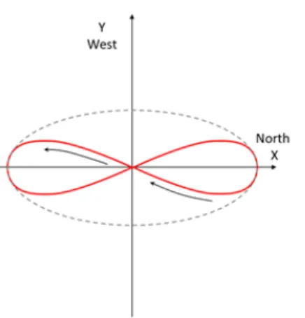
Figure 4.
In a steadily tilting camera together with the laboratory frame, the orbit shape looks like a lemniscate. The trace of the vertical at the same x -value as the bob is superimposed with the X -axis. The angles between the orbit and the X-axis at the origin are the respective peak precession angles for the first half and the second half of the pendulum cycle respectively. So the precession angle is described by a cosine function. Similarly, the extreme curvatures of the orbit are those of a tangent ellipse at both ends, but with alternate senses. There follows a sinusoidal behaviour of the ellipticity, or of the axis ratio b/a , thus in quadrature with the precession oscillation.
However, in the image coordinates of the inertial camera at the ceiling, the center of attraction at the alidade level constantly recedes westward from the bob, resulting in an ever increasing torque applied to the pendulum. In order to calculate that gravitational torque, note that the extremity of the horizontal component of the gravitational acceleration parallel to the Y -axis describes an inverse-cosine trajectory as a function of the x-coordinate of the bob (Figure [3]).
The first order perturbation equation for the tilt angle reads ϑ ¨
(1)+ ω
12ϑ
(1)= gΩt
l = ω
o2Ωt, (= ω
o2Ωt cos λ) for the latitude λ. (3.14) The particular solution of the differential equation, considering the initial conditions, is
ϑ
(1)= Ωt, After t = T /4,
lϑ
(1)(T /4) = Ωl ω
o(π/2) ≈ 1.57|b|,
It is seen that the ever increasing lateral acceleration due to tilt deflects the oscillation plane toward the positive Y -values by more than the negative b-value of the constant-tilt situation. The inertial trajectory in free space becomes the cuspid zigzag of Figure [3]. This can be compared to the inertial view of the ellipse generated by constant tilt (dashed black curve). The closing action of this third stage of the experiment consists in letting the laboratory follow the Earth rotation velocity Ω for the subsequent cycles. The open trajectory of Figure [3] is then transformed into the closed orbit of Figure [4].
This equatorial experiment shows that the (in general elliptic) orbit type generated by a
constant tilt angle belongs to the usual family of trochoid curves describing the spherical
pendulum. The orbit as a whole undergoes no precession, as one normally expects for a Foucault
pendulum at the equator. However, a spherical pendulum at the equator is characterised not by a
constant tilt angle, but by a constant rate of change of tilt angle. Consequently, a drastic departure
from the ellipse is induced by the rate of change of tilt angle. A new orbit type not belonging to the
trochoid family is generated. It turns out to be the pedal curve of a family of elongated hyperbolas
with foci on the X-axis and with the scale of the Y -axis multiplied by ω/Ω. A special case of
13
rspa.ro y alsocietypub lishing.org Proc R Soc A 0000000 .. .. .. .. .. .. .. .. .. .. .. .. .. .. .. .. .. .. .. .. .. .. .. .. .. .. .. .. ..
such a pedal curve with hyperbolic asymptotes at 90
◦to each other is the well-known Bernouilli lemniscate (see animation on Wikipedia [27]).
A practical way of interpreting that orbit type may be as follows. Note that the scale of the Y- axis in Figure [4] has been greatly exaggerated for the sake of clarity: in fact, the pedal curve is very elongated along the X -axis. Near the end of the swing where ϑ rapidly increases to its maximum value a/l, ϕ ≈ 0 and ϕ ˙ ≈ 0. The corresponding focus of the pedal curve practically coincides with the focus of an ellipse, so that the arc of the new orbit is very close to an ellipse arc at the end of its semi-major axis. Once that extremal arc has been described, as the bob passes past the focus of the very elongated asymptotic ellipse, one already has ϑ ≈ 0. The ever receding attraction point initiates the inward departure from the ellipse in the direction of the ellipse center, which is reached after one quarter-cycle. As the center is crossed, the attraction direction is reversed, thus creating an inflection point at the origin and the onset of the second quarter-cycle symmetrically to the first one, but in reverse order. Contrary to the elliptic orbit, the asymptotic ellipse arc at the other extremity of the swing is described in the reverse sense, preparing the second half-cycle centrally symmetric to the first one.
(d) New Berry phases
According to the above mathematical treatment, the alternating precession angle (and alternating precession rate) within an oscillation cycle is the immediate consequence of the rate of tilt. Its amplitude amounts to half the angular difference between the two tangents to the orbit of Figure [4] crossing at the origin. It is also worth mentioning that the amount of alternating precession is a consequence of the gravitational torque applied to the tilted pendulum. But the scale of the Y -axis of that figure is directly proportional to the duration of the period. Hence the amount of alternating precession per cycle is directly proportional to the period and also to cos λ, as mentioned in Equation [3.14]. So, considering the constant tilt rate Ω of the vertical at the equator, in free space, the half-cycles separately cumulate the geometrical phases −π rad and +π rad respectively. The algebraic sum of the half-cycle precession angles cumulates zero geometrical phase at the equator, in accordance with the observed Foucault pendulum behaviour and with Hannay’s result [12].
At the equator, a normal gyroscope whose axis parallel to the equator would be re-positioned parallel to the equatorial plane after each infinitesimal time increment would tend to cumulate, in the precession angle ψ, a geometric phase of 2π rad per Earth revolution. If the gyroscope axis is parallel to the polar axis, it is the spin angle ϕ that cumulates the geometric phase 2π. With a pendulum oscillating in the North-South direction, one half-cycle gyroscope would cumulate a precession angle of π rad, since it is active for half the Earth-revolution time, while the other one would cumulate −π rad. So,
the cumulative algebraic difference of the two half-cycle geometric phases for each cycle constitutes a novel geometric phase that amounts to 2π rad per Earth revolution.
At a given latitude λ, that cumulative geometric phase difference between the two elementary gyroscopes sums up to 2π cosλ. In analogy with the standard Berry phase of the Foucault pendulum, which has been described as the result of the elementary phase increments accumulated by a two-form corresponding to the two orthogonal circular eigenstates of the pendulum [10,12], it can similarly be argued that the Berry phase due to the tilt rate of the vertical can be represented by a two-form corresponding to the normal states of two contra-spinning gyroscopes acting alternately during each complete pendulum cycle.
So far, the above treatment of the gyroscopic effects of tilt rate of the Foucault pendulum at the equator has been made for a tilt rate direction perpendicular to the N-S swinging azimuth.
Note that the precession angle ψ of the tangent plane to the orbit of Figure [1] simply becomes
the swing azimuth when the orbit is rectilinear or very slightly elliptic. However, due to the fast
flip of 180
◦at the end of each half-cycle, ψ discriminates between the odd- and even half-orbit
azimuths. Since there is no net precession per cycle at the equator, a pendulum with azimuth
14
rspa.ro y alsocietypub lishing.org Proc R Soc A 0000000 .. .. .. .. .. .. .. .. .. .. .. .. .. .. .. .. .. .. .. .. .. .. .. .. .. .. .. .. ..
ψ mod 180
◦still accumulates the Berry phase 2π cos ψ, while a single gyroscope would become unstable once its axis has become perpendicular to the equator. Then, the Berry phase is no longer cumulated in ψ, but in ϕ, which causes no gyroscopic effect.
Out of the equator, Foucault precession ensures a steady variation of ψ. So, the tilt-rate Berry phase per cycle is time dependent through the the time dependence of ψ. The net precession rate in each half-cycle is given by the two expressions
Ψ ˙
evenodd
= Ω
2 (− sin λ ± cosλ cos ψ) , (3.15)
Their sum gives the Foucault rate and their difference gives the peak-to-peak alternating rate. For a typical latitude of 35
◦and a N-S swinging azimuth, the peak-to-peak alternating rate reaches 140% of the Foucault rate.
Figure [5] shows the odd (red) and even (blue) half-cycle precession rates of the Gifu pendulum, together with their algebraic sum (in green). Despite the obvious occurrence of numerous perturbations in tilt rate, the nature of the pedal orbit of figure [4] is confirmed by the neatly separated precession rates of each half-cycle of oscillation. The gyroscopic tilt-rate effect effectively turns out to be of the same order as the Foucault effect itself for that latitude of 35.43
◦N. In particular, approximately every 6 hours (or every 45
◦in azimuth), the combined precession angle of the cycle is totally provided by the odd half-cycle precession alone.
Figure 5.
Half-cycle precession rates (red and blue) for an 18-hour Foucault pendulum experiment at Gifu University, Gifu, Japan, during a solar eclipse on July 21, 2009. Eclipse maximum corresponds to the elapsed time 5.4h. The total precession angle per cycle (green) is also given. The large-scale and rather smooth variations of the total precession rate are satisfactorily explained by conventional classical theories on pendulum anisotropy (Kamerlingh Onnes) and on nonlinear response to finite amplitudes (Airy). On the contrary, the differential precession rate showing the gyroscopic effects appears to reveal a
very significant first order structure that cannot be attributed to any known varying tilt rateor, equivalently, to any known changes in horizontal acceleration components. The dashed curves show the expected values from gyroscopic theory for the latitude of Gifu.
(e) Experimental evidence of the novel pedal-curve orbit
Among several meticulous Foucault pendulum experiments conducted by the author since 2001
[14], few have been completely exploited, due to the lack of programming facility, in those years,
to address the many technical difficulties related to data streams involving several millions of
high definition video frames filling a 1.5-terabyte hard disk. However, the Japanese expedition
of July 2009 has been sufficiently processed so far to enable the elaboration of Figure [5]. The
physical setup consisted of an 8 m long, 1 mm diameter piano wire attached to a concrete beam
at the ceiling of a concrete bunker and supporting a 12 kg low drag lenticular bob. Bob motion
was indeed recorded via a high-definition camera placed near the suspension point, thanks to a
15
rspa.ro y alsocietypub lishing.org Proc R Soc A 0000000 .. .. .. .. .. .. .. .. .. .. .. .. .. .. .. .. .. .. .. .. .. .. .. .. .. .. .. .. ..
pattern of small retroreflecting stickers on the bob and on the surrounding fixed alidade. A small 5-volt LED flashlight next to the camera provided so much brightness from the retroreflecting markers that the ambient lighting appeared black through the small lens-aperture setting used [16]. At the post-processing stage, 60 bob positions per second were imported into an EXCEL file where the various orbit parameters were computed. The values of the major and minor axes could be determined to ±15 µm and the azimuths to ± meridian pass20" of arc at the beginning and ±5’ of arc at the end. The bob was launched at the amplitude of 145 mm (0.018 rad) by the burnt-thread method from a post at the geographic azimuth 305
◦, hence with the odd half-cycles running roughly in the NW-SE direction. It was planned that the Foucault precession rate would bring the swinging azimuth along the local meridian after 6 hours, namely by the time of eclipse meridian passage in Gifu (11 minutes before eclipse maximum). The achieved level of precision allowed dependable data to be recorded even after 18 hours, as the swinging amplitude was merely 10 mm. By that time, the swinging azimuth had rotated by 180
◦.
It is also worth mentioning, in accordance with the above-presented gyroscopic theory of the Foucault pendulum, that the tilt effect should affect the precession angle ψ most markedly when the direction of tilt-rate change is orthogonal to the swing azimuth, while it should be non observable when the direction of tilt change is parallel to the swing azimuth. In this latter case, indeed, the geometrical Berry phase is applied to the spin angle ϕ instead of the precession angle ψ. As a matter of fact, considering the launch azimuth and the unexpected precession acceleration due to anisotropy and nonlinearity, the swing direction has become meridian after 5.4 hours, then zonal or East-West 10.6 hours later. Accordingly, the separation of the odd and even curves is maximal at 5.4 hours while it is essentially zero 16 hours after launch.
During the first hour, a decaying transient alternating precession rate starting at twice the theoretical value seems to be the result of the unavoidable initial high-frequency nodding oscillation. Nodding is due to the retaining thread not being perfectly aligned with the center of mass of the bob-wire assembly before the starting burn out. Since that frequency is not commensurable with the pendulum frequency, some residual nodding rate is left over in the same direction for a sequence of several half-cycles while the swinging motion changes direction.
Therefore, even if that nodding does not influence the total precession rate on the average, it is nevertheless sharply detected as a tilt-rate perturbation.
Finally, in so far as gyroscopic theory of the pendulum is concerned, the result of Equation [3.15] for the Gifu pendulum is shown as the red (lower dashed) sine curve for the odd half-cycle and the blue (upper dashed) sine curve for the even half-cycle. However, the very significant higher-frequency structure of the differential precession rate in Figure [5], as compared to the theoretical periodicity of Equation [3.15], could be an indication that alternating precession rate is not merely governed by the revolution of the Earth, but might also be due to other causes that still need proper investigation.
4. Discussion
Right away, it is interesting to note that, at such mid-latitude, as long as the swing azimuth lies in a grossly N-S direction, the alternating precession rate is of the same order as the Foucault rate. For this particular case in the Northern hemisphere, Foucault precession essentially turns out to be only provided by the odd half-cycle. Obviously, that would be less the case when approaching the pole. On the contrary, near the equator, the half-cycle separation would increase to a maximum whereas the Foucault rate approaches zero.
It is customary that experimenters who use the Foucault pendulum to demonstrate effects
related to celestial bodies (eclipse effects, tide effects, syzygies) look for anomalies in precession
rate that are not explicable by known pendulum theories. It is beyond the scope of the present
article to expose in detail how the particular pendulum used in this work complies with those
16
rspa.ro y alsocietypub lishing.org Proc R Soc A 0000000 .. .. .. .. .. .. .. .. .. .. .. .. .. .. .. .. .. .. .. .. .. .. .. .. .. .. .. .. ..
theories.
1Suffice it to say that the changes in total precession rate that are implied from those theories are very smooth. They are at most responsible for the broad structure of the total precession rate (green) in Figure [5].
As mentioned above, this 18-hour experiment was performed as an attempt to verify an eventual Foucault pendulum response to a solar eclipse. The pendulum was launched six hours and eleven minutes before eclipse maximum, which was partial at 81% in Gifu. Oddly enough, Figure [5] shows a grossly time symmetrical deviation pattern from Equation [3.15] centered around the timestamp 5.4h, which is the time of meridian passage of the eclipse. The maximum deviations from theory occur at 2.2 hours before and after meridian passage. Of course, the two contrarotating gyroscopes react in opposite directions, so that a mere second order unbalance proves observable as an eventual eclipse effect in conventional total precession, albeit hardly emerging above noise level. Indeed, the very weak indentations at elapsed times 4h and 7h could be claimed as anomalies, in as much as their signal level stands above noise.
It is not clear whether the initial transient is really due to nodding or if it would be an influence of swing amplitude upon alternating precession rate amplitude. More research needs to be done in order to ascertain any effect of swing amplitude on the alternating precession rate. From looking at Figure [5], it seems feasible to admit a decaying time constant of the order of 2h for that transient. So, if one makes abstraction of that decaying phenomenon, it becomes more and more evident that another pair of anomalous deviations occur at about 4.4h before and after meridian passage.
Finally, a similar anomaly is observable 2.2h before anti-meridian passage, namely at 15.2h, but in the opposite sense with respect to the theoretical curve. Moreover, contrary to the case of meridian passage where the peak-to-peak alternative precession rate, apart from a small offset, is exactly as predicted by the gyroscopic theory, there is a sharp anomalous peak in alternating precession rate exactly at the time of anti-meridian passage (17.4h) while gyroscopic theory predicts nearly zero alternating precession rate. In case this could be of any interest for future research, it may be noted that, for July 21, the Sun-Moon zenith angle in Gifu is 15.4
◦southwards at meridian passage (syzygy Earth-Pendulum-Moon-Sun) and 129.2
◦northwards at anti-meridian passage (syzygy Pendulum-Earth-Moon-Sun).
On the other hand, it is expected that the tilt rate of the the local vertical should not be constant when considering the trajectory of the pendulum in free space. Since the pendulum bob, contrary to its suspension point, is not rigidly attached to the Earth surface, it is subject to the laws of inertia in such a way that the linear accelerations and linear decelerations of the Earth center along its translation around the Sun, due to its rotation about the Earth-Moon barycenter, are translated into varying tilt rates for the pendulum. The order of magnitude of those tilt-rate variations is
271of the Earth rotation tilt rate. Consequently, deviations of the order of 3 % from the cosine law of equation [3.15] should be detectable in alternating precession rate, if the noise level is low enough.
This low noise condition does not seem to be fulfilled in the present case.
Incidentally, it might be interesting to note that Latham and Last have already measured the precession rate fluctuations of a high performance gyro-compass during a solar eclipse in Peru [30,31]. They did observe a pseudo-periodical pattern similar to that of Figure [5], with gross periodicities around 1.2h and 6h, but with compensating torque amplitudes of only ~10
−4times the compensating torque required by Earth rotation. They also simultaneously measured the variations in direction of g’. These add up to about 0.6%, weakly correlated with the gyro-compass torque, while the noise level stands at about 0.3%.
For the time being, it is not yet clear whether the large deviations observed in Figure [5] are a form of low-frequency noise or the result of some cosmological phenomenon. The apparent regularity of the time sequence pattern speaks in favor of some organized causal source. If the gyroscopic response of the Foucault pendulum really unveils a cosmological event, the sensitivity
1A companion article is in preparation, where it will be shown how KO theory and Airy theory apply to this particular pendulum implementation, together with a thorough analysis of this and similar experiments with the anisosphere model [29].