HAL Id: ineris-03246714
https://hal-ineris.archives-ouvertes.fr/ineris-03246714
Submitted on 2 Jun 2021
HAL is a multi-disciplinary open access
archive for the deposit and dissemination of
sci-entific research documents, whether they are
pub-lished or not. The documents may come from
teaching and research institutions in France or
abroad, or from public or private research centers.
L’archive ouverte pluridisciplinaire HAL, est
destinée au dépôt et à la diffusion de documents
scientifiques de niveau recherche, publiés ou non,
émanant des établissements d’enseignement et de
recherche français ou étrangers, des laboratoires
publics ou privés.
oxidative potential at a city scale (Grenoble, France) –
Part 1: Source apportionment at three neighbouring
sites
Lucille Joanna S. Borlaza, Samuël Weber, Gaëlle Uzu, Véronique Jacob,
Trishalee Cañete, Steve Micallef, Cécile Trébuchon, Rémy Slama, Olivier
Favez, Jean-Luc Jaffrezo
To cite this version:
Lucille Joanna S. Borlaza, Samuël Weber, Gaëlle Uzu, Véronique Jacob, Trishalee Cañete, et al..
Disparities in particulate matter (PM10) origins and oxidative potential at a city scale (Grenoble,
France) – Part 1: Source apportionment at three neighbouring sites. Atmospheric Chemistry and
Physics, European Geosciences Union, 2021, 21 (7), pp.5415 - 5437. �10.5194/acp-21-5415-2021�.
�ineris-03246714�
https://doi.org/10.5194/acp-21-5415-2021 © Author(s) 2021. This work is distributed under the Creative Commons Attribution 4.0 License.
Disparities in particulate matter (PM
10
) origins and
oxidative potential at a city scale (Grenoble, France) –
Part 1: Source apportionment at three neighbouring sites
Lucille Joanna S. Borlaza1, Samuël Weber1, Gaëlle Uzu1, Véronique Jacob1, Trishalee Cañete1, Steve Micallef4, Cécile Trébuchon4, Rémy Slama5, Olivier Favez2,3, and Jean-Luc Jaffrezo1
1University Grenoble Alpes, CNRS, IRD, INP-G, IGE (UMR 5001), 38000 Grenoble, France 2INERIS, Parc Technologique Alata, BP 2, 60550 Verneuil-en-Halatte, France
3Laboratoire Central de Surveillance de la Qualité de l’Air (LCSQA), 60550 Verneuil-en-Halatte, France 4Atmo Auvergne-Rhônes Alpes, 38400 Grenoble, France
5IAB, Team of Environmental Epidemiology applied to Reproduction and Respiratory Health,
University of Grenoble Alpes, 38000 Grenoble, France
Correspondence: Lucille Joanna Borlaza (lucille-joanna.borlaza@univ-grenoble-alpes.fr) and Jean-Luc Jaffrezo (jean-luc.jaffrezo@univ-grenoble-alpes.fr)
Received: 2 November 2020 – Discussion started: 10 December 2020 Revised: 4 March 2021 – Accepted: 5 March 2021 – Published: 8 April 2021
Abstract. A fine-scale source apportionment of PM10 was
conducted in three different urban sites (background, hyper-center, and peri-urban) within 15 km of the city in Greno-ble, France using Positive Matrix Factorization (PMF 5.0) on measured chemical species from collected filters (24 h) from February 2017 to March 2018. To improve the PMF solution, several new organic tracers (3-MBTCA, pinic acid, phthalic acid, MSA, and cellulose) were additionally used in order to identify sources that are commonly unresolved by classic PMF methodologies. An 11-factor solution was obtained in all sites, including commonly identified sources from primary traffic (13 %), nitrate-rich (17 %), sulfate-rich (17 %), industrial (1 %), biomass burning (22 %), aged sea salt (4 %), sea/road salt (3 %), and mineral dust (7 %), and the newly found sources from primary biogenic (4 %), secondary biogenic oxidation (10 %), and MSA-rich (3 %). Generally, the chemical species exhibiting similar temporal trends and strong correlations showed uniformly distributed emission sources in the Grenoble basin. The improved PMF model was able to obtain and differentiate chemical profiles of spe-cific sources even at high proximity of receptor locations, confirming its applicability in a fine-scale resolution. In or-der to test the similarities between the PMF-resolved sources, the Pearson distance and standardized identity distance
(PD-SID) of the factors in each site were compared. The PD-SID metric determined whether a given source is homogeneous (i.e., with similar chemical profiles) or heterogeneous over the three sites, thereby allowing better discrimination of lo-calized characteristics of specific sources. Overall, the addi-tion of the new tracers allowed the identificaaddi-tion of substan-tial sources (especially in the SOA fraction) that would not have been identified or possibly mixed with other factors, re-sulting in an enhanced resolution and sound source profile of urban air quality at a city scale.
1 Introduction
Atmospheric aerosols, or particulate matter (PM), are com-plex mixtures of particles from direct and indirect emissions (e.g., gas-to-particle conversion processes) that are from nat-ural and anthropogenic sources in the atmosphere (Wilson and Spengler, 1996). The growing interest in ambient aerosol studies is driven by their impacts on health, air quality, and global climate (Colette et al., 2008; Horne and Dab-dub, 2017; McNeill, 2017; Shiraiwa et al., 2017). Numer-ous epidemiological studies have established consistent as-sociations between PM and various health diseases,
espe-cially cardiorespiratory illnesses (Brunekreef, 2005; Fran-chini and Mannucci, 2009; Langrish et al., 2012; Ostro et al., 2011; Willers et al., 2013). Once inhaled, PM notably has the capacity to generate reactive oxygen species (ROS), which leads to pro-inflammatory responses that can ultimately re-sult in apoptosis (Ayres et al., 2008; Jin et al., 2018; Nel, 2005; Piao et al., 2018; Yang et al., 2018). Investigating the PM oxidative potential (OP) in light of its major emission sources in various urban environments can then provide valu-able information to instigate air pollution abatement policies limiting health outcomes. However, spatially resolved PM source apportionment at a city scale remains a challenging task (Dai et al., 2020a, b; Pandolfi et al., 2020).
Receptor models demonstrated their ability to extract in-formation by variable reduction techniques, especially in large datasets, in different branches of scientific research. In particular, the Positive Matrix Factorization (PMF) model is widely used in many studies to determine the contribution of emission sources in PM, based on the characterization of chemical tracers in a series of PM samples (Belis et al., 2014, 2020; Hopke, 2016; Pindado and Perez, 2011; Saeaw and Thepanondh, 2015; Weber et al., 2019). The option of re-fining source profiles by adding constraints have further im-proved the accuracy of identifying sources (Charron et al., 2019; Marmur et al., 2007; Weber et al., 2019; Zhu et al., 2018), especially when specific chemical species and unique tracers are included (Bullock et al., 2008; Wang et al., 2017b; Yan et al., 2017; Zhang et al., 2010). In fact, the PMF model has shown good strengths in both rural and urban environ-ments (Pindado and Perez, 2011; Schauer and Cass, 2000); however, there are limited studies in cities at a fine-scale res-olution that allows the assessment of local variabilities in a metropolitan area.
The city of Grenoble (France), with a complex topography and marked seasonal cycles of particulate pollution, offers interesting opportunities to explore the capability of PMF to resolve both the small spatial and large temporal scales of variabilities of the contribution of PM sources with the possibility of using additional tracers. Specific meteorologi-cal conditions, topography, and lometeorologi-cal sources impact the lo-cal PM chemistry in the atmosphere thereby requiring ad-ditional sources to properly scrutinize these local variations in urban environments. Further, previous works were already conducted in the area using extended PMF (Srivastava et al., 2018b; Weber et al., 2019), providing useful benchmark in-dicators.
The application of PMF requires to accurately consider a wide range of chemical components in PM, particularly for its organic fraction (Seinfeld and Pankow, 2003), consist-ing of complex mixtures especially in urban environments (Schauer and Cass, 2000; Zheng et al., 2004). In fact, around 80 % of organic matter (OM) generally remains unidentified at the molecular level (Chevrier, 2016; Golly et al., 2019) re-sulting in misclassification or several unapportioned sources of PM10. Additionally, the difference in formation pathways
of PM components may limit the identification of sources of PM, especially the secondary organic carbon (SOC) fraction, without the use of relevant organic tracers (Srivastava et al., 2018b; Wang et al., 2017b). Different organic tracers have already been integrated in previous PMF studies, allowing resolution of specific sources of organic aerosols that cannot be easily identified, such as primary biogenic aerosols and products of secondary processes in the atmosphere (Waked et al., 2014; Belis et al., 2019; Golly et al., 2019; Hu et al., 2010; Weber et al., 2019).
In particular, Srivastava et al. (2018b) were able to dif-ferentiate between different types of primary and secondary organic fractions at a Grenoble urban background site, af-ter analysing about 150 organic markers (and selecting 25 of them for the final PMF run). Such studies are highly labour-intensive and often require the use of costly analytical de-vices and methods, whereas some of the missing key molec-ular markers might still be obtained using simpler and/or more targeted techniques. Moreover, the usefulness of these organic tracers in PMF analysis requires extensive method-ological exploration, in terms of their applicability as source tracers considering the much lower variability of their con-centrations compared to other traditional tracers.
In this paper, we present results of a study conducted over 1 year at three sites within 15 km of each other in the Greno-ble metropolitan area within the framework of the Mobil’Air project (available in https://mobilair.univ-grenoble-alpes.fr/, last access: 2 November 2020). The sources of PM10 were
apportioned considering major chemical components con-tributing to the PM mass, including organic and elemental carbon, ions, a condensed set of commonly used organic markers (anhydride monosaccharides, polyols, MSA), and metals. Additional fit-for-purpose tracers, including free cel-lulose and several organic acids, were also added in the PMF input datasets to tackle specific sources that are difficult to discriminate using a traditional PMF dataset only. Results obtained from this improved PMF analysis were then used to investigate the spatial and seasonal variabilities in the source contributions for different urban typologies inside a metropolitan area. The overall outputs of this study could be of interest to policy makers in providing vital informa-tion for designing effective particulate matter control strate-gies including the setup of low emission zones and an op-portunity to acquire more knowledge about the associations of these emissions with other emerging health-based metrics (e.g., OP of PM) at a city scale as presented in the companion paper (Borlaza et al., 2021).
2 Methodology
2.1 PM10sample collection
The metropolitan area of Grenoble, regarded as the capital of the French Alps, has a population of about 440 000
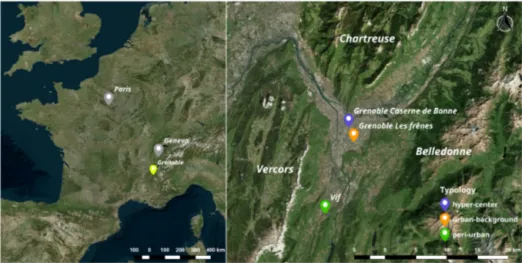
inhabi-Figure 1. Grenoble, the city where the sampling was made, placed on a European map (left), and PM monitoring sites (right): Les Frênes or LF (background), Caserne de Bonne or CB (hyper-center), and Vif (peri-urban). Image credit: Bing™Aerial. © Microsoft.
tants. The city itself presents a low altitude range (between 204 and 600 m a.s.l.) but is located in an alpine environment (Fig. 1), surrounded by several mountain ranges, including Chartreuse (north), Vercors (south and west), and Belledonne (east). These mountains restrict the movement of air heavily affecting the local meteorology and favouring the develop-ment of atmospheric temperature inversions with entrapdevelop-ment of pollutants in the valley, particularly in the winter (Bessag-net et al., 2020). The topography within the Grenoble basin and seasonality of particulate air pollution in the city makes it an ideal location to explore both the small- and large-scale variabilities of PM sources During this study, a PM10
sampling campaign was conducted in the Grenoble area at three sites selected to represent various urban typologies, in-cluding Les Frênes (LF, urban background site, 214 m a.s.l.), Caserne de Bonne (CB, urban hyper-center, 212 m a.s.l.), and Vif (peri-urban area, 310 m a.s.l.). These sites are all within a 15 km range from the city center. LF is a long-standing reference urban background site for the regional air quality monitoring network (Atmo Auvergne Rhône-Alpes), nearby a park at the outer fringe of the city. Vif is a peri-urban site, with suburban housings close to rural areas. However, this site could potentially receive industrial emissions from a nearby chemical industrial area (< 6 km) in the air flux within this north–south valley. Substantial influence of bio-genic emissions could also be expected as this site is in between the foot of Vercors and Belledone national parks. Lastly, while in a pedestrian area, the site of CB is in the hyper-center of Grenoble and exposed to traffic emissions from the nearby boulevards.
The daily (24 h) PM10 sampling collection was
con-ducted from 28 February 2017 to 10 March 2018 (start-ing at 00:00 LT) with an average 3 d sampl(start-ing interval. A total of 125, 127 and 127 samples were collected during this year-long campaign at LF, CB, and Vif, respectively.
The PM10collection was performed using high-volume
sam-plers (Digitel DA80, 30 m3h−1) onto 150 mm-diameter pure quartz fibre filters (Tissu-quartz PALL QAT-UP 2500 diam-eter 150 mm). All filter-handling procedures of filters were strictly under quality control assurance procedures to avoid any possible contamination. In particular, filters were pre-heated at 500◦C for 12 h before use to avoid organic con-tamination. At least 20 field blank filters were collected at each site to determine detection limits (DL) and to check for the absence of contamination during sample transport, setup, and recovery. After particle collection, filter samples were wrapped in aluminium foil, sealed in zipper plastic bags, and stored at < 4◦C until further chemical analysis. Complemen-tary measurements at the sampling sites notably included the total PM10 mass concentration measured using tapered
ele-ment oscillating microbalances equipped with filter dynam-ics measurement systems (TEOM-FDMS) (Grover, 2005). 2.2 Classical set of chemical analyses
Sampled filters were subjected to various chemical analyses for the quantification of the major chemical constituents and specific chemical tracers of sources needed for PMF studies. The carbonaceous fractions (organic carbon (OC) and ele-mental carbon (EC)) were analysed with a Sunset Lab anal-yser (Aymoz et al., 2007; Birch and Cary, 1996) using the EUSAAR2 thermo-optical protocol (Cavalli et al., 2010). To-tal organic matter (OM) in daily ambient aerosols were esti-mated by multiplying the OC mass by a fixed conversion fac-tor of 1.8 based on findings obtained from previous studies (Favez et al., 2010; Putaud et al., 2010).
A solid/liquid extraction was performed on 11.34 cm2 punches soaked in a 10 mL of ultra-pure water under vor-tex agitation for 20 min. The extract was then filtered with a 0.25 µm porosity Acrodisc (Milipore Millex-EIMF) filter. The major ionic components were measured by ion
chro-matography (IC) following a standard protocol described in Jaffrezo et al. (1998) and Waked et al. (2014), using an ICS3000 dual-channel chromatograph (Thermo-Fisher) with AS11HC column for the anions and CS12 for the cations. This technique allowed the quantification of sodium (Na+), ammonium (NH+4), potassium (K+), magnesium (Mg2+), calcium (Ca2+), chloride (Cl−), nitrate (NO−3), sul-fate (SO2−4 ), and methane sulfonic acid (MSA).
Furthermore, anhydro-sugars and saccharides were anal-ysed by high-performance liquid chromatography with pulsed amperometric detection (HPLC-PAD), using a Thermo-Fisher ICS 5000+ HPLC equipped with 4 mm di-ameter Metrosep Carb 2 × 150 mm column and 50 mm pre-column in isocratic mode with 15 % of an eluent of sodium hydroxide (200 mM) and sodium acetate (4 mM) and 85 % water, at 1 mL min−1. This method notably allowed the quantification of anhydrous saccharides (levoglucosan and mannosan), polyols (arabitol and mannitol), and glucose as tracers of biomass burning and primary biogenic aerosols (Samaké et al., 2019b; Waked et al., 2014).
Finally, major and trace elements were analysed after min-eralization of a 38 mm diameter punch of each filter, using 5 mL of HNO3(70 %) and 1.25 mL of H2O2 during 30 min
at 180◦C in a microwave oven (microwave MARS 6, CEM). The analysis of 18 elements (Al, As, Ba, Cd, Cr, Cu, Fe, Mn, Mo, Ni, Pb, Rb, Sb, Se, Sn, Ti, V, and Zn) was per-formed on this extract using inductively coupled plasma mass spectroscopy (ICP-MS) (ELAN 6100 DRC II PerkinElmer or NEXION PerkinElmer) in a way similar to that described by (Alleman et al., 2010).
The procedures for filter sampling and chemical analyses have been performed following the recommendations of re-lated EN standards (i.e., EN 12341, EN 14902, EN 16909, EN 16913) (Favez et al., 2021). Moreover, quality control of the chemical speciation analyses includes chemical mass closure as presented in Sect. S2. It should also be noted that our group successfully participates in regular inter-laboratory comparison exercises for OC and EC within ACTRIS and in EMEP (European Monitoring and Evaluation Programme) for ions analysis.
2.3 Additional set of analyses of organic tracers 2.3.1 Organic acids
The analysis of a large array of organic acids (including pinic and phthalic acids, and 3-MBTCA) was conducted using the same water extracts as for IC and HPLC-PAD analyses. In brief, this was performed by HPLC-MS (GP40 Dionex with a LCQ-FLEET Thermos-Fisher ion trap), with nega-tive mode electrospray ionization. The separation column is a Synergi 4 µm Fusion – RP 80A (250 × 3 mm ID, 4 µm par-ticle size, from Phenomenex). An elution gradient was op-timized for the separation of the compounds, with a binary solvent gradient consisting of 0.1 % formic acid in
acetoni-trile (solvent A) and 0.1 % aqueous formic acid (solvent B) in various proportions during the 40 min analytical run. Col-umn temperature was maintained to 30◦C. Eluent flow rate
was 0.5 mL min−1, and injection volume was 250 µL. Cali-brations were performed for each analytical batch with solu-tions of authentic standards. All standards and samples were spiked with internal standards (phthalic-3,4,5,6-d4 acid and succinic-2,2,3,3-d4acid). The calculation of the final atmo-spheric concentrations was corrected with the concentrations of internal standards and of the procedural blanks, taking also into account the extraction efficiency varying between 76 % and 116 % (depending on the acid).
2.3.2 Cellulose
The concentration of cellulose within PM10 samples was
quantified based on a protocol improving the procedure pro-posed by Kunit and Puxbaum (1996). Cellulose was ex-tracted from the filter in an aqueous solution, which was then processed in several solutions of enzymes in order to break-down the cellulose into glucose units. Resulting glucose con-centration was quantified using an HPLC-PAD technique. To do so, a 21 mm diameter punch was first extracted for 40 min using an ultrasound bath in 3 mL of an aqueous solution with thymol buffer (pH 4.8). Then two enzymes solutions (cellu-lase (Sigma Aldrich, C2730) with 20 µL of an aqueous solu-tion at 70 units g−1) and glucosidase (Sigma Aldrich, 49291), with 60 µL of an aqueous solution at 5 units g−1) are added into the solution. The solution was then incubated at 50◦C for 24 h for the hydrolysis to occur. The hydrolysis is stopped by placing the solution in an oven at 100◦C for 45 min. The solution was then centrifuged (7000 rpm) for 15 min, and carefully extracted out using a syringe before being analysed with an HPLC-PAD instrument. The procedural blanks are greatly improved when the enzymes stock solutions are fil-tered to lower their glucose content. This is performed with a series of cleaning steps (n = 10) by tangential ultrafiltration in a Vivaspin 15R tube at 7000 rpm in Milli-Q water.
The HPLC-PAD (Dionex DX500) is equipped with a Metrohm column (250 mm long, 4 mm diameter), with an isocratic run of 40 min with the eluents A (50 %, 18 mM NaOH), B (25 %, 100 mM NaOH + 150 mM NaAc), and C (25 %, 220 mM NaOH). Column temperature is maintained at 30◦C. Eluent flow rate is 1 mL min−1, and injection vol-ume is 250 µL. Each analytical batch also includes standard glucose solutions as well as standard cellulose solutions (us-ing 20 µm beads, Sigma Aldrich, S3504) that have been pro-cessed like the real samples in order to determine the spe-cific efficiency of the cellulose-to-glucose enzymatic conver-sion for each batch. The final calculation of the atmospheric concentration of the free cellulose takes this conversion effi-ciency into account. It varied according to the batch, gener-ally ranging from 65 % to 80 %. The calculation of the cellu-lose concentration also takes into account the initial concen-trations of atmospheric glucose of each sample, determined
in parallel with the HPLC-PAD analysis of sugars and poly-ols as described above. Finally, field and procedural blanks are also taken into account.
2.4 Source apportionment 2.4.1 PMF input dataset
Source apportionment of PM10 was conducted using the
United States Environmental Protection Agency (US-EPA) software PMF 5.0 (Norris et al., 2014), aiming at the identifi-cation and quantifiidentifi-cation of the major sources of PM10for the
three urban sites in the Grenoble basin. Briefly, PMF is based on the factor analysis technique (Paatero and Tapper, 1994) applying a weighted least-squares fit algorithm allowing the resolution of Eq. (S1) (in the Supplement). In our study, 35 chemical species were used as input variables, namely OC∗, EC, ions (Na+, K+, NH+
4, Mg
2+, Ca2+, NO− 3, SO
2−
4 and
Cl−), trace metals (Al, As, Cd, Cr, Cu, Fe, Mn, Mo, Ni, Pb, Rb, Sb, Se, Sn, Ti, V and Zn) and organic tracers (MSA, levoglucosan, mannosan, polyols (sum of arabitol and man-nitol), pinic acid, 3-MBTCA, phthalic acid, and cellulose), as summarized in Table S1 in the Supplement. We assumed that arabitol and mannitol originated from the same source, and hence combined them into one component labelled as “polyols” (Samaké et al., 2019a). In order to avoid double counting of carbon mass, OC∗ was calculated as the differ-ence between total OC and the quantity of C atoms contained in the different organic markers included in the PMF input data matrix (as detailed in Eq. S2). The uncertainties of the input variables were calculated using Eq. (S3) (Gianini et al., 2012). Finally, the species displaying a signal-to-noise ratio (S/N ) lower than 0.2 were discarded and those with S/N between 0.2 and 2 were classified as “weak” variables (and then down-weighted applying 3-fold uncertainties).
2.4.2 Set of constraints
Since mixing issues between factors are inherent to PMF (i.e., collinearity due to meteorological conditions) and to possible rotational ambiguity in the solution, we applied a set of constraints to the selected best base case solutions thanks to the ME-2 solver (Paatero, 1999). The constraints used were similar to that of Weber et al. (2019), who applied a minimum set of constraints to a large series of data sets within the SOURCE program. We also added specific con-straints for the traffic factor, derived from a previous study in Grenoble dedicated to traffic emissions (Charron et al., 2019), as summarized in Table 1. These constraints were ap-plied similarly to the data sets from the three sites. This al-lows the orientation of the PMF solution towards more stable and environmentally realistic profiles.
2.4.3 Criteria for a valid solution
Solutions with a total number of factors between 7 and 12 were tested for the determination of the base cases. During factor selection, the Q/Qexp ratio (< 1.5), the geochemical
interpretation of the factors, the weighted residual distribu-tion, and the total reconstructed mass were evaluated. Finally, the optimal solutions obtained for each urban site was sub-jected to error estimation to ensure stability and accuracy of the solutions, using displacement (DISP) and bootstrapping (BS) methods. The DISP analysis evaluates that no swap-ping had occurred in any of the factors. Solutions with > 80 out of 100 BS mapped factors were considered appropriate solutions. The final retained optimal solutions after the ap-plication of constraints fulfilled the recommendations of the European guide on air pollution source apportionment with receptor models (Belis et al., 2014). The sensitivity of the so-lutions to the applied constraints was also carefully evaluated by comparison between the base and constrained cases. More information about the source apportionment methodology is provided in the SI.
2.4.4 Similarity assessment
A test of similarity between source profiles, based on their specific chemical relative mass composition at each site, was performed by comparing the Pearson distance (PD) and stan-dardized identity distance (SID). This allows the evaluation of the variability of the solutions across these different ur-ban environments. The PD and SID were calculated using Eq. (S4) (Belis et al., 2015).
The PD metric represents the sensitivity of a chemical pro-file based on the differences in the major mass fractions of PM, whereas the SID represents the sensitivity to all compo-nents (hence taking into account trace species). Homogenous profiles that are stable over different site types are expected to have PD < 0.4 and SID < 1.0 (Pernigotti and Belis, 2018). Conversely, factors outside of this range are considered to have heterogeneous profiles.
2.4.5 Estimation of the contribution uncertainties The BS profiles uncertainties for the obtained solutions are presented in Sect. S3, in the form of mean±std of the 100 BS for all sites. As PMF5.0 does not directly output this to the user, we provided an estimate of the contribution uncertain-ties based on the method presented in Weber et al. (2019). During the BS estimation, both the G and F matrices are available; however, only the F matrix is given back to the user (the G matrix being used internally to map the differ-ent profiles). Hence, the daily contributions of each of the species are estimated using
XBSi =Gref×FBSi, (1)
where FBSi is the profile of the bootstrap i, and XBSi is the
contribu-Table 1. Summary of the applied chemical constraints on source-specific tracers in the PMF factor profiles.
Factor profile Element Type Value
Biomass burning Levoglucosan Pull up maximally (% dQ 0.50)
Biomass burning Mannosan Pull up maximally (% dQ 0.50)
Primary biogenic Levoglucosan Set to zero 0
Primary biogenic Mannosan Set to zero 0
Primary biogenic Polyols Pull up maximally (% dQ 0.50)
Primary biogenic EC Pull down maximally (% dQ 0.50)
MSA-rich MSA Pull up maximally (% dQ 0.50)
MSA-rich Levoglucosan Set to zero 0
MSA-rich Mannosan Set to zero 0
MSA-rich Polyols Pull down maximally (% dQ 0.50)
MSA-rich EC Pull down maximally (% dQ 0.50)
Nitrate-rich Levoglucosan Set to zero 0
Nitrate-rich Mannosan Set to zero 0
Mineral dust Ti Pull up maximally (% dQ 0.50)
Primary traffic Levoglucosan Set to 0 0
Primary traffic Mannosan Set to 0 0
Primary traffic∗ Cu Pull up maximally (% dQ 0.50)
Primary traffic∗ Fe Pull up maximally (% dQ 0.50)
Primary traffic∗ Sn Pull up maximally (% dQ 0.50)
Primary traffic∗ Ca2+ Pull down maximally (% dQ 0.50)
Primary traffic Cu/Fe Set to value 0.046 (% dQ 0.50)
Primary traffic Cu/Sn Set to value 5.6 (% dQ 0.50)
Primary traffic Cu/Sb Set to value 12.6 (% dQ 0.50)
Primary traffic Cu/Mn Set to value 5.7 (% dQ 0.50)
Primary traffic OC∗/EC Set to value 0.44 (% dQ 0.50)
∗Only applied in the Vif (peri-urban) site.
tion Grefand the bootstrap run FBSi. Similarly, the DISP
con-tribution uncertainties are given by the reference concon-tribution G multiplied by the lower and upper limits of the DISP result for each species.
3 Results and discussion
3.1 General evolution of concentrations of PM10and
chemical species
The daily PM10 mass concentrations at the three
measure-ment sites, determined with the TEOM-FDMS for the dates of filter sampling, ranged from 3 to 61 µg m−3with an over-all average of 14 ± 9 µg m−3 during the sampling period. Average PM10 levels were the highest at the urban
hyper-center site (CB) (16 ± 10 µg m−3), followed by the urban background site (LF) (14 ±8 µg m−3), and the peri-urban site (Vif) (13 ± 9 µg m−3). Annual averages of PM10 mass
con-centrations and chemical compositions at all sites and at in-dividual urban sites are shown in Table S2. The sites in this study showed minimal exceedances of the current PM10
Eu-ropean limit value of 40 µg m−3(3.7 %, 1.6 %, and 1.6 % of measurement days at the LF, CB, and Vif sites, respectively). Most of these exceedances occurred during the winter season
indicating the necessity to additionally implement season-specific regulations for PM10 emission reductions. Organic
matter (OM) was the largest contributor in PM10 and
ac-counted for 54 %, 51 %, and 56 % of mass concentration on an annual basis in LF, CB, and Vif, respectively. This was followed by contributions from the major inorganic species (NH+4, NO−3, and SO2−4 ), suggesting strong influence from secondary inorganic aerosol (SIA) that are generally asso-ciated with long-range transport of pollutants or the occur-rence of a small-scale thermal inversion within the Grenoble basin. An extensive description of the PM10chemistry in the
Grenoble basin has already been presented in Srivastava et al. (2018b) for the years 2013–2014 at the LF site. Our re-sults showed notable similarities for most chemical species for the year 2017–2018, especially in terms of seasonal varia-tions and respective contribution of chemical species to PM10
mass concentrations. Therefore, we will only describe these aspects briefly in this paper.
First, the time series analysis of PM10 and its chemical
composition in the Grenoble basin during the sampling pe-riod showed mild to strong seasonal trends. Part of it can be attributed to the atmospheric dynamics in the area given its alpine environment resulting in atmospheric temperature in-versions that are especially common in winter. In the absence of strong winds during the winter season (especially during
anti-cyclonic periods), higher concentrations of air pollutants could be expected. Indeed, PM10concentrations were higher
during the colder months (October to April) with an average of 17±10 µg m−3and lower during the warmer months (May to September) with an average of 10 ± 4 µg m−3.
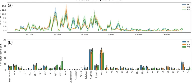
We observed a strong seasonality for some chemical species with higher concentrations during the colder months including OC∗, EC, K+, NO−3, NH+4, levoglucosan, man-nosan, and phthalic acid. These species are commonly asso-ciated with primary emissions during the process of biomass burning (OC, EC, K+, levoglucosan, mannosan) and sec-ondary atmospheric processing (NO−3, NH+4, phthalic acid). Alternatively, specific species with higher concentrations during warmer months include MSA, polyols, 3-MBTCA, and pinic acid. These species are known to be products of a wide range of photochemical reactions in the atmo-sphere partly formed by OH-initiated oxidation (Atkinson and Arey, 1998; Szmigielski et al., 2007) and can be ex-plained by enhanced photochemical production due to an in-crease in temperature-dependent hydroxyl radical (OH) centration. A summary of temporal evolutions of the con-centration for some species including SO2−4 , Cu, cellulose, polyols, 3-MBTCA, pinic acid, and phthalic acid is shown in Fig. 2.
Second, the Pearson correlation coefficients of the tem-poral evolution of each species across sites is presented in Fig. 3. Similarity of temporal trends and strong correlations of PM10 components between our three sites indicates the
influence of large-scale transport processes or possible uni-form distribution of some emission sources in the Grenoble area. Further, the accumulation and removal processes of the PM may be driven by similar season-specific environmen-tal conditions at a local scale. A strong correlation was ob-served in OC∗, EC, ions, polyols, levoglucosan, mannosan, 3-MBTCA, phthalic acid, and pinic acid between sites sug-gesting similar origins and atmospheric processes affecting the concentrations of these species. The three sites seem to be equally impacted by long-range transport since concentration of SO2−4 appears almost identical. We also clearly see rela-tively similar temporal trends for the organic acids (MSA, pinic, and 3-MBTCA). Notably, we also observed an impor-tant episode in phthalic acid in late February 2018 affect-ing all the three sites. An extensive discussion on the forma-tion processes of anthropogenic SOA in high-concentraforma-tion events was already provided in Srivastava et al. (2018b). However, this new observation brings in the hypothesis that these processes may take place specifically due to heteroge-neous chemistry when associated with fog episodes, as can be observed by local web cams over the city (discussed in answers to reviewers). Conversely, cellulose and most metal species showed weak to mild correlations between sites, pos-sibly indicating that the sources of these species are highly localized, with a potential impact that is variable at a city scale. Particularly, cellulose presents similar order of magni-tude at the three sites but presents higher concentration at CB,
Table 2. Summary of PMF-resolved sources and their specific trac-ers.
Identified factors Specific tracers
Biomass burning Levoglucosan, mannosan, K+, Rb, Cl− Primary traffic EC, Ca2+, Cu, Fe, Sb, Sn
Nitrate-rich NO−3, NH+4
Sulfate-rich SO2−4 , NH+4, Se
Mineral dust Ca2+∗, Al, Ti, V
Sea/road salt Na+, Cl−
Aged sea salt Na+, Mg2+
Industrial As, Cd, Cr, Mn, Mo, Ni, Pb, Zn
Primary biogenic Polyols, cellulose
MSA-rich MSA
Secondary biogenic oxidation 3-MBTCA, pinic acid
∗
Vif site did not have high loadings ofCa2+species in this factor.
especially during winter. A few metals only showed strong correlations between LF and CB but not with Vif, such as Al, Cu, Fe, Rb, and Sb, which are tracers of road transport activity or biomass burning emissions. Specifically, Cu con-centrations are similar at the three sites during summer but present significantly lower concentration in Vif compared to the two urban sites of CB and LF during winter.
3.2 PM10source apportionment
In the following sections, a description of the best PMF so-lution obtained after application of constraints is provided for each of the three sites, together with a discussion about the factors that are associated with the added organic trac-ers (MSA, polyols, cellulose, pinic and 3-MBTCA acids). The presentation of error estimations, chemical profiles, and temporal evolutions of the PMF-resolved sources, and the discussion about the more classical factors can be found in Sect. S3.
3.2.1 General description of the solutions
The PMF model was applied independently on the data set of each three sites, using 35 chemical atmospheric compounds in each site. The constrained solutions for each site consist of 11 factors, including common factors such as primary traf-fic, biomass burning, nitrate-rich, sulfate-rich, aged sea salt, sea/road salt, and mineral dust. Also, with the use of biogenic tracer species, we identified a primary biogenic factor and a MSA-rich factor. These factors are similarly determined in Weber et al. (2019) for each of 15 sites in France. We also de-termined a metal-rich factor, identified as an industrial factor, accounting for a very small part of the PM10 mass. Finally,
using new organic proxies (pinic and 3-MBTCA acids), we identified a secondary biogenic oxidation factor that is rarely described in other PMF studies. Table 2 shows a synthesis of the tracers used to identify these 11 PMF-resolved factors that are found at each of the three sites.
Figure 2. Temporal evolutions of (a) phthalic acid, (b) pinic acid, (c) 3-MBTCA, (d) MSA, (e) polyols (arabitol + mannitol), (f) cellulose, (g) SO2−4 and (h) Cu in the three urban sites in the Grenoble basin (LF in orange, CB in blue, and Vif in green).
Figure 3. Concentration time series Pearson correlation coefficient of PM10and its chemical composition between LF and CB (LF-CB), LF and Vif (LF-Vif), and CB and Vif (CB-Vif).
Other solutions with fewer or greater number of factors were also investigated but these solutions were less defined, and factor merging was often observed. The reconstructed PM10 contributions from all sources with measured PM10
concentration showed very good mass closure in all sites (LF: r = 0.99, n = 125, p < 0.05; CB: r = 0.99, n = 126, p <0.05; and Vif: r = 0.99, n = 126, p < 0.05) indicating very good model results.
This result is in line with a previous study in the city of Grenoble (Srivastava et al., 2018b) but with slight improve-ments in the PM10mass closure (from r = 0.93 to r = 0.99).
A complete comparison of the PMF-resolved sources be-tween the two studies is presented and discussed in Sect. S4. The two sets of results are in good agreement, despite the samples being collected 4 years apart. There were several identified sources that are similar in both studies such as biomass burning, primary traffic, mineral dust, aged sea salt, sulfate- and nitrate-rich (identified collectively as secondary inorganics in Srivastava et al., 2018b), and primary biogenic (identified as fungal spores and plant debris in Srivastava et al., 2018b). Additionally, due to a number of differences in the input variables used, there are some sources that are
completely unique to each study. In particular, the sources that we have uniquely identified are industrial, sea/road salt, MSA-rich, and secondary biogenic oxidation sources. Con-versely, Srivastava et al. (2018b) have uniquely identified two SOA sources: biogenic SOA and anthropogenic SOA. It can be argued that the secondary biogenic oxidation source (11 %) in our study and the biogenic SOA (12 %) in Srivas-tava et al. (2018b) are in some way similar, although differ-ent tracers were used to iddiffer-entify them. Particularly, Srivas-tava et al. (2018b) identified the biogenic SOA source with high contributions from α-methylglyceric acid (α-MGA and 2-methylerythritol (2-MT) that are isoprene oxidation ucts and hydroxyglutaric acid (3-HGA), an oxidation prod-uct from α-pinene. On the other hand, our study identified the secondary biogenic oxidation source with high contri-butions from 3-MBTCA and pinic acid (essentially from α-pinene oxidation). While not uniquely identified in our study, the contributions of phthalic acid in several common anthropogenic-derived sources (sulfate- and nitrate-rich) can also mark the potential contributions from anthropogenic SOA sources. Finally, the considerable economic advantage in the specific organic tracers used in our study, in terms of the type of chemical analyses performed, could assist future studies utilizing organic species in PMF.
It is also important to note that, although still in the ac-ceptable range, the sulfate-rich factor obtained in our PMF results yielded the most BS unmapped factors amongst the PMF-resolved factors (up to 25 % for the CB site). This may be the sign of possible mixing of different processes/sources in this factor.
3.2.2 PM10contribution
Biomass burning (17 %–26 %), sulfate-rich (16 %–18 %), and nitrate-rich (14 %–17 %) sources were the highest con-tributors to the total PM10 mass on a yearly average in the
Grenoble basin. Primary traffic (12 %–14 %) and secondary biogenic oxidation (8 %–11 %) sources also contributed a relevant amount. Figure 4 presents a comparison of the source contributions in each site based on mass concentra-tion (in µg m−3). These results are in line with recent studies leading to anthropogenic and SOA sources heavily influenc-ing urban air pollution in western Europe (Daellenbach et al., 2019; Golly et al., 2019; Pandolfi et al., 2020; Srivastava et al., 2018b; Weber et al., 2019). The most notable difference across all sites is the sharp decrease in mineral dust in Vif compared to the other two urban sites, and this is discussed further in Sect. 3.4.1.
3.2.3 MSA-rich
This factor is identified with a high loading of MSA, a known product of oxidation of dimethylsulfide (DMS), commonly described as resulting from marine phytoplankton emissions (Chen et al., 2018; Li et al., 1993). Other chemical species
with significant concentrations in this factor include sulfate and ammonium. Although a very useful tracer of marine bio-genic sources, MSA showed in our series only weak to mild correlations with ionic species from marine aerosols such as Na+(r: 0.2–0.3) and Mg2+(r: 0.3–0.4). This suggests poten-tial emissions originating from terrestrial biogenic sources instead, which has been similarly suggested before (Bozzetti et al., 2017; Golly et al., 2019), and/or from forest biota (Jar-dine et al., 2015; Miyazaki et al., 2012). On an annual scale, this factor accounted for 2 %–4 % of the total mass of PM10
and shows a strong seasonality with highest contributions during summer, reaching up to 53 %, 57 %, 52 % of the total PM10mass on some specific days in LF, CB, and Vif,
respec-tively. The similarity in the temporal distribution across sites, as shown in Fig. S3.8, especially the summer peaks, could be linked to the influence of long-range transport of pollutants in the MSA-rich factor.
3.2.4 Primary biogenic
The primary biogenic factor was identified with high load-ings of both polyols and cellulose (see Fig. 5). Polyols (rep-resented by the sum of arabitol and mannitol) are known as tracers of primary biological aerosols from fungal spores and microbes (Bauer et al., 2002; Igarashi et al., 2019). Poly-ols has been used in several studies as a tracer of biogenic sources, contributing in France within a range of 5 %–9 % of PM10 on a yearly average (Samaké et al., 2019b; Srivastava
et al., 2018b; Waked et al., 2014; Weber et al., 2019). Cellu-lose is a potential macro-tracer for plant debris from leaf litter and seed production (Kunit and Puxbaum, 1996; Puxbaum, 2003) that is very rarely used in source apportionment studies as of today. It can represent a large fraction of the PM mass in the coarse mode (Bozzetti et al., 2016), and it represents up to 6 % during the warm season in the Vif site.
A strong correlation was found in the temporal evolution of polyols across the three sites in our study indicative of large-scale impact of sources for these species (Samaké et al., 2019b). Conversely, cellulose concentrations present only weak correlations across the three sites, possibly indicating that the influence of the sources of this species might be more local. Although polyols and cellulose are both tracers of primary biogenic sources, only a rather mild correlation (r = 0.5) was found between these two tracers, with season-ality of their concentrations being slightly different (Fig. 2). It shows that the processes and the sources are probably dis-tinct for the two sets of chemical species. However, the PMF is not able to separate them, and this factor includes most of the cellulose (58 %, 51 %, and 74 % in LF, CB, and Vif, respectively), and also most of the polyols (99 %, 90 %, and 83 % in LF, CB, and Vif, respectively). The remaining frac-tion of cellulose concentrafrac-tions was included in the mineral dust factor in LF and CB, and in the primary traffic factor in Vif, suggesting the possibility of resuspension processes for this compound (see the SI for details). We can also note that
Figure 4. Factor contributions in µg m−3for the three sites (LF: blue, CB: orange, Vif: green). Bar plots depict the mean annual value and the standard deviation of daily variations.
Figure 5. Primary biogenic factor for the three urban sites. (a) Contribution to PM10given the mean and standard deviation of the 100 BS. (b) Percentage (%) of each species apportioned by this factor (dots refer to the constrained run, bar plots refer to the mean, and error bars refer to the standard deviation of the 100 BS).
the cellulose was not at all apportioned in the biomass burn-ing factor, an indication that it may not be emitted by this source.
Despite their slightly different origins, the PMF analysis captures the combined contribution of polyols and cellulose to a factor that can be termed “primary biogenic sources”. In this study, this factor accounted for 3 %–4 % of the total mass of PM10on an annual scale, and a strong seasonality was
ob-served, with up to 18 % (in LF), 8 % (in CB), and 17 % (in Vif) of the total PM10mass on average in summer, with
spe-cific days reaching up to 60 % of PM10 for example at the
Vif site (see Fig. 5). These temporal variations are consistent with higher biological activity (increased production of fun-gal and fern spores and pollen grains) in this season due to increase in temperature and humidity (Graham et al., 2003; Verma et al., 2018). This may also be attributed to an in-creased plant metabolic activity (production of plant debris
from decomposition of leaves) and the proximity to forested and agricultural areas of the sampling sites (Gelencsér et al., 2007; Puxbaum, 2003). Finally, one can note that the chem-ical profiles also include some fractions of the tracers from secondary biogenic production (3-MBTCA and pinic acid), indicative of some degree of mixing between primary and secondary biogenics.
3.2.5 Secondary biogenic oxidation
The secondary biogenic oxidation factor was identified with high loadings of 3-MBTCA and pinic acids (see Fig. 6). Both tracers of this factor are known to be products of secondary oxidation processes of alpha-pinene from various biogenic origins. As suggested by the nearly identical mass fraction determined in Srivastava et al. (2018b) at the same site, this factor may also contain some PM resulting from the
oxida-Figure 6. Secondary biogenic oxidation factor for the three urban sites. (a) Contribution to PM10given the mean and standard deviation of the 100 BS. (b) Percentage (%) of each species apportioned by this factor (dots refer to the constrained run, bar plots refer to the mean, and error bars refer to the standard deviation of the 100 BS).
tion of isoprene epoxydiols (IEPOX) (Surratt et al., 2010; Zhang et al., 2017) that may present a rather similar season-ality (Budisulistiorini et al., 2013, 2016), but this is still an open question.
The apportionment of such a factor is not commonly achieved in receptor modeling using offline tracers (van Drooge and Grimalt, 2015; Heo et al., 2013; Hu et al., 2010; Srivastava et al., 2018a). On an annual scale in our study, this factor accounted for 8 %–11 % of the total mass of PM10,
but can be as high as 58 % (11 µg m−3) on specific days (see Fig. 6a). The strong correlation between 3-MBTCA and pinic acids suggests similarity of origin of the secondary biogenic oxidation factor in the Grenoble area, despite inter-site corre-lations for 3-MBTCA (older oxidation state of alpha-pinene, hence more homogeneous at the city scale) being larger than that for pinic acid (former oxidation product, less homoge-neous). Although significant portions (56 %–72 %) of these species (3-MBTCA and pinic acids) are in this secondary biogenic oxidation factor, there are still relevant contribu-tions in other factors, including primary biogenic, sulfate-and nitrate-rich, aged sea salt, sulfate-and MSA-rich. Conversely, the presence of phthalic acid contribution in this factor (around 10 % of its concentration), which could be emitted directly from biomass burning or formed during secondary process-ing from anthropogenic emissions (Hyder et al., 2012; Klein-dienst et al., 2007; Wang et al., 2017a; Yang et al., 2016), also suggests that this factor has anthropogenic influence. All of these indicate that the PMF process did not deliver a pure secondary biogenic oxidation factor, either due to data
pro-cessing limitation or because of real mixing of these sources in the PM.
3.3 Re-assignment of factors thanks to the new proxies 3.3.1 Importance of the new proxy for factor
identification
With the use of these additional organic tracers, there are sev-eral added information drawn from the results of the PMF model. First, the notable contributions of phthalic acid in sev-eral sources could further confirm the mixing influence of anthropogenic processes in various sources of PM10such as
sulfate- and nitrate-rich but also with secondary biogenic ox-idation sources. Second, adding 3-MBTCA and pinic acids in the input variables allowed the identification of a significant secondary biogenic oxidation factor that is generally diffi-cult to identify with PMF studies of offline samples. Com-parisons already started with the factors obtained by AMS studies (Vlachou et al., 2018), but more work remains to be done in order to evaluate their proper correspondence. 3.3.2 Comparison with a “classic” PMF solution In order to quantify the added value and the changes brought in by the additional tracers, a reference PMF using a chem-ical dataset (not including cellulose, pinic acid, phthalic acid, and 3-MBTCA) and parameters similar to that in the SOURCES project (Weber et al., 2019) was performed, here-after called “classic”, and the results were compared with those from the present study (called “orga”). Figure 7 shows
Figure 7. Mean annual contribution (µg m−3) of PMF-resolved factors of PM10in the Grenoble basin using a classic set of input variables similar to SOURCES (“classic”) and using additional new organic tracers (“orga”).
the comparison of the yearly average mass contribution of the different factors for these two approaches. A detailed com-parison of chemical profiles between the “classic” and “orga” PMF runs in each site is summarized in Sect. S3. One can see that most observations below are consistent in all three sites. Some factors remain unaffected or only marginally mod-ified: it is the case for the biomass burning source with a percentage increase in contribution, only ranging from 1 % to 14 %, in the “orga” compared to the “classic” PMF run across all sites. The primary biogenic source also posed an interesting case with a minimal decrease in contribution at 0.1 % and 6 % in the LF and CB sites, respectively. However, adding more specific biogenic tracers changed the contribu-tion of the primary biogenic factor in Vif, from 1.1 µg m−3 for the “classic” PMF down to 0.50 µg m−3 for the “orga” PMF run, a value that is much more in line with the contribu-tions observed at the other sites (0.56 and 0.55 µg m−3in CB and LF, respectively). This further highlights the usefulness of the additional organic tracers (e.g., addition of cellulose in the primary biogenic factor), especially for specific site typologies.
Conversely, the most impacted factor is the sulfate-rich one, to a similar extent for the three sites with a much higher mass fraction in the “classic” PMF run in large part due to higher loadings of OC∗. It may indicate possible merg-ing with organic aerosol sources in the “classic” PMF, as presented in a comparison of chemical profiles between the “classic” and “orga” PMF runs in each site summarized in Sect. S3. Figure 7 shows that the differences are really close to the content of the new secondary biogenic oxidation fac-tor. Secondary aerosols, such as the sulfate-rich factor, can be transported over long distances and can remain in the at-mosphere for about a week (Warneck, 2000), allowing them to interact with numerous other species and undergo differ-ent atmospheric oxidation processes. In fact, several studies have investigated various oxidation pathways of sulfate-rich
sources (Barker et al., 2019; Ishizuka et al., 2000; Schnei-der et al., 2001; Ullerstam et al., 2002, 2003; Usher et al., 2002). In the SPECIEUROPE database, several studies have reported sulfate-rich sources influenced by a variety of differ-ent fuel combustion sources (Bove et al., 2014; Pernigotti et al., 2016; Pey et al., 2013). It is, therefore, not surprising that part of the matter in the sulfate-rich source was re-assigned to different other sources upon addition of the organic tracers in the “orga” PMF run. A comparable study in Metz (France) also used another organic tracer (oxalate) to apportion a sec-ondary organic aerosol (SOA) source from PM, ascribing it possibly to both biogenic and anthropogenic emissions (Petit et al., 2019).
We also observed an increase in the contributions of the MSA-rich factor at the three sites, with an increase in con-tributions from specific inorganic species, such as SO2−4 and NH+4 (see Fig. S3.8.1). Conversely, a decrease in contribution from polyols was observed in the chemical profile of primary biogenic factor in Vif (see Fig. S3.7.1). Results show that in the “classic” PMF run, the contribution of polyols was almost completely assigned to the primary biogenic factor (> 94 % of its total mass). On the other hand, the “orga” PMF run re-sulted in a contribution of polyols to the MSA-rich factor of about 10 % of its total mass.
Finally, there is also an observed re-assignment of the Ca2+species that further refined specific factors in Vif. The mineral dust factor is often identified with high loadings of Ca2+; however, this is not the case for Vif, particularly for the “classic” PMF run (less than 1 % of total Ca2+, al-though attached with important uncertainties). It is important to note that Ca2+in an urban environment can come from several sources such as construction activities and global re-suspended dust from various activities (from biomass burn-ing and traffic). Previous studies comparburn-ing measurements at LF and a site close to a highway (2 km apart) showed a 34 % increment of this factor near the highway, supporting
the influence of resuspended dust with traffic (Charron et al., 2019). With the addition of the organic tracers, there was an observed increase in the contribution of Ca2+in the mineral dust factor in Vif (see Fig. S3.11.1), resulting in more than 20 % of the total Ca2+apportioned in this factor (a value is still attached with important uncertainties). Interestingly, the contribution of Ca2+is mainly transferred from the primary traffic factor to the mineral dust factor. This resulted in a de-creased contribution of the primary traffic factor in Vif from 2.4 µg m−3for the “classic” PMF down to 1.8 µg m−3for the “orga” PMF run. Again, this is a value closer to the contri-butions at the other sites (2.0 and 1.8 µg m−3in CB and LF, respectively) (see Fig. S3.2.1).
3.3.3 Decrease in uncertainties
Another advantage of adding specific proxies in the PMF is the lowering of uncertainties associated with some other chemical species in some factors. Indeed, we observed a de-crease in the BS uncertainties, notably for the OC∗and also for some main tracers of sources in several profiles (see in the SI (S3)). The sulfate-rich is the most impacted factor when adding the new organic tracers and the higher uncertainties in the “classic” PMF run provided insights that this profile may have some internal mixing. Splitting this factor, thanks to the new organics, refined the sulfate-rich factor and strengthened the BS stability of this factor, decreasing the BS uncertain-ties.
Concerning the DISP, the range of uncertainties was also narrowed for 74 % of the species in factors when compar-ing the “classic” and “orga” PMF. This decrease in uncer-tainties for the DISP when adding new variables was already observed by (Emami and Hopke, 2017), but our study addi-tionally observed this in the BS error estimation. Overall, on top of being able to identify new factors, the addition of the new specific proxies in the PMF strengthened the confidence we have for all other factors.
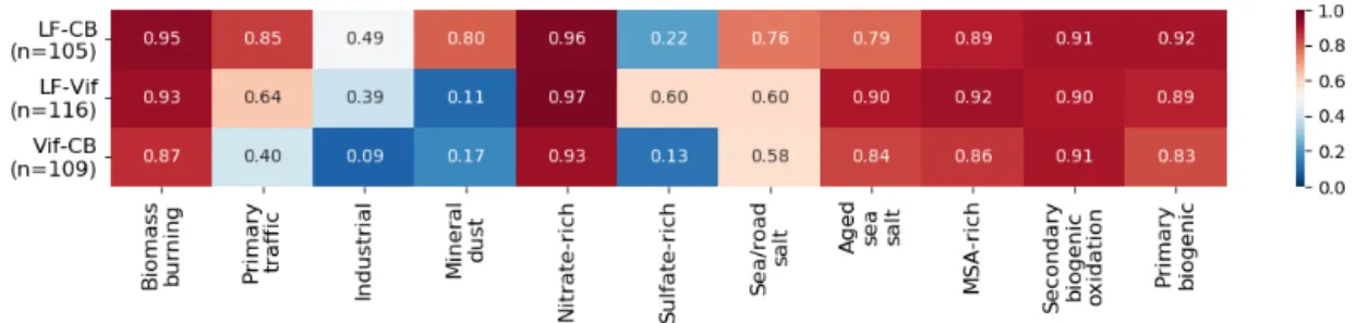
3.4 Fine-scale variability of the temporal contribution Figure 3 indicates correlations of the concentrations for many chemical species across the sites. Additionally, the tempo-ral evolution of the contribution of commonly resolved fac-tors are further investigated in this section. Figure 8 presents the Pearson correlation coefficient of the contributions of the sources for the three pairs of sites. The sources that resulted in consistently strong correlations (r > 0.77) across all sites are biomass burning, nitrate-rich, aged sea salt, MSA-rich, secondary biogenic oxidation, and primary biogenic sources. The sea/road salt factor showed good correlations across the sites with a correlation coefficient ranging from 0.58 to 0.76. Factors with strong seasonality appeared to be highly cor-related between sites (biomass burning, nitrate-rich, MSA-rich, and primary biogenic). This tends to affirm that such factors are dominated either by large-scale transport (i.e.,
nitrate-rich) or by a strong climatic determinant. It is interest-ing to note that the primary biogenic factor presents system-atically a slightly lower correlation than the polyols (LF-CB: rpolyols=0.94 to rprimary biogenic=0.91, LF-Vif: rpolyols=
0.92 to rprimary biogenic=0.88 and Vif-CB: rpolyols=0.87 to
rprimary biogenic=0.82). This may suggest a secondary
pro-cess or a combination of several different primary propro-cesses in the primary biogenic factor affecting the sites at differ-ent rates (Petit et al., 2019; Samaké et al., 2019b). We also clearly see a stronger similarity between the two urban sites (LF and CB) compared to the peri urban one, notably for the primary traffic, mineral dust, and, to a lower extent, the industrial factor. This may be explained not only by the prox-imity of the location of the two former sites within the city, but also by their similarity in typology compared to the peri-urban site type in Vif. However, there are two factors that do not present good correlation between all sites.
One of them is the sulfate-rich factor which presents a sim-ilar contribution when comparing LF and Vif but low to no correlation when compared to CB. A deeper analysis shows that the sulfate-rich, together with the nitrate-rich factor in CB, explains a large part of the winter spike of secondary in-organics (23/24 Feburary 2018), whereas in LF and Vif only the nitrate-rich factor explains most of it. This spike drives the Pearson correlation coefficient to a low value and, with-out it, the correlation increases drastically (see Fig. S5.1 for the full scatterplot). Some PMF solutions of the BS in LF and Vif also had this behavior but were not chosen as the “best” solution. We propose two hypotheses for this differ-ence: (1) during winter, some heterogeneous chemistry may take place in fog episodes in the Grenoble basin (resulting in episodic spikes in the SO2−4 contribution) that may not be spatially homogeneous at a city scale, leading to mixing of secondary sources, and (2) we have reached the limit of the PMF methodology to de-convolute further the secondary in-organics. Both hypotheses may be concurrent.
A further indication of a potential mixing between the sulfate- and nitrate-rich factors is presented in Fig. S5.3. In this figure, the total mass concentration of PM and major ions (SO2−4 , NO−3, and NH+4) were compared between sites when the sulfate- and nitrate-rich factors were combined. Strong correlations between sites were found indicating similarity of such concentrations in secondary sources. It is out of scope of this work to determine whether this is a limitation of the PMF approach or whether there are some processes leading to real differences. We note however that apart from these spikes, the SO2−4 apportioned by this factor at three sites are in good agreement, and are within the uncertainties of each other (see Fig. 9). This figure also highlights that the uncer-tainty for the SO2−4 in this factor is higher for the CB site, as also shown in the chemical profile in Fig. S3.6.
The second factor which showed low correlations between pairs of sites is mineral dust, specifically when comparing Vif to the two other sites. This is in line with the difference in the PM10apportioned by this factor as shown in the previous
sec-Figure 8. Heat map of the time series Pearson correlation coefficient of all factor contributions between LF and CB (LF-CB), LF and Vif (LF-Vif), and CB and Vif (CB-Vif).
Figure 9. SO2−4 apportioned by the sulfate-rich factor at the three sites, according to the uncertainties given by the 100 BS as shown by the mean (solid line) and the standard deviation (shaded area).
tion. However, a closer look at the contribution scatterplot of VifMineral dustvs. CBMineral dust(see Fig. S5.2) highlights that
some events are very close to the 1 : 1 line. This is indicative of two regimes for mineral dust, with differences due to some specificity in the atmospheric dynamics in the valley near the surface. To investigate it further, a potential source contribu-tion funccontribu-tion (PSCF) analysis of the mineral dust factor for the Vif and CB sites was performed in order to assess the ori-gin of air masses of this factor (Fig. 10). For the Vif site, the main origin is Spain, with well-defined air flow canalized by the valley and katabatic flows in a south-to-north direction (a phenomenon also reported in Largeron and Staquet, 2016). On the other hand, the origin for CB is not as well-defined. These PSCF pattern tends to indicate that the sources of the mineral dust factor present a strong local component for the urban sites (CB and LF being very similar), while the origin of the mineral dust factor in Vif appears to be mainly affected by long-range transport of dust only.
3.5 Fine-scale variability of chemical profiles
An additional similarity test was also performed to investi-gate the fine-scale variabilities of the chemical profiles of the factors. A similarity analysis at a regional scale in France identified stable chemical profiles obtained by PMF stud-ies across many sites, corresponding to biomass burning, sulfate-rich, nitrate-rich, and fresh sea salt factors (Weber et
al., 2019). In our study, a parallel analysis was performed in order to evaluate the stability of the chemical profiles of the identified factors in high-proximity receptor locations. Briefly, PMF-resolved sources were compared for each pair of sites using both PD and SID to obtain a similarity metric (PD-SID).
3.5.1 (Dis-)similarity of the chemical profiles at the three sites
Figure 11 presents the similarity plot (PD-SID) obtained for the 11 factors found in this study. The biomass burning fac-tor yielded the most stable chemical profile in all the sites in the Grenoble basin, which is consistent. Other stable factors include sulfate- and nitrate-rich, primary biogenic, MSA-rich, and secondary biogenic oxidation. The industrial and sea/road salt factors, both marginally above the accepted PD metric, could be considered as having heterogeneous profiles based on the contributions of these sources to the total PM10
in each site.
However, a clear heterogeneous chemical profile was found in the mineral dust, this further emphasized the dif-ference in origin of this factor as previously discussed in Sect. 3.4. More details about of the chemical profile of this factor can be found Fig. S3.11. One of the main differences is the lack of OC∗in the Vif site compared to LF and CB sites, together with a much lower Ca2+contribution. Additionally,
Figure 10. The PSCF analysis of the days with a mineral dust loading higher than 0.4 µg m−3for the CB site (a) and Vif (b). Darker shades indicate higher probability density of source origin.
Figure 11. Similarity plot of all chemical profiles in each site. The shaded area (in green) shows the acceptable range of the PD-SID metric. For each point, the error bars represent the standard devia-tion of the three pairs of comparisons.
there is a lower SO2−4 apportioned in the mineral dust factor in Vif. The only similarity between all the sites are the high loadings of Al, Ti, and V as well as important contributions from other crustal metals (Fe, Ni, Mn). It also has to be noted that the cellulose is present up to about 20 % of its total mass in the mineral dust profile in the CB site; however, the BS es-timates indicate very important uncertainties for this species in this factor (see Fig. S3.11).
Surprisingly, the sulfate-rich factor chemistry is one of the most stable profiles, although its temporal contributions ex-hibit high spatial variation, notably at CB compared to the LF and Vif sites.
Finally, although the primary traffic factor showed a stable profile based on the similarity plot (PD-SID metric), it has to be noted that, in the reference run (i.e., constrained), the species concentrations are within the BS uncertainties for all species at LF and CB sites but outside the BS range for the Vif site (see Fig. 12). Notably, the BS predicted higher con-tribution from Cu, Fe, Sb and Sn, which are common trac-ers of tyre and brake wear, than the reference run. Addition-ally, the Ca2+is overestimated in the reference run by a large amount, as well as the OC∗, and, to a lesser extent, the
recon-structed PM10. Such BS results indicate that, in Vif, the
pri-mary traffic factor is heavily influenced by this phenomenon on specific days, which has led to an overestimation of the total PM10 apportioned by this factor. Additionally, even at
low concentrations, some terrestrial elements (Al, As, Ti) and cellulose are present in the primary traffic factor. As a result, even if the primary traffic characteristic of this factor is dominant, the influence of road dust re-suspension is not negligible for this factor in Vif.
3.5.2 Comparison with other chemical profiles of PM10
sources from a regional study
It is interesting to evaluate whether a PMF study conducted at a city scale is leading to more similar source chemical pro-files than a study using a database from a much larger area. Another question is whether PMF can produce more simi-lar chemical source profiles with the help of additional or-ganic tracers than a “classic” PMF run. Hence, the results obtained here are compared to those in the SOURCES pro-gram (Weber et al., 2019) for the nine factors common in both studies (the secondary biogenic factor was not iden-tified in the SOURCES program with the data sets not in-cluding its proper chemical tracers). This can be represented with the projection on a similarity plot of the distances be-tween the factors for the three pairs of sites over the Grenoble basin, both for the “classic” and “orga” PMF. This is com-pared to the results from all possible pairs of sites within the 15 sites of the SOURCES study (distributed over France), mapped with a probability density function of similarities. Figure 13 presents these plots for the factors “primary traf-fic” and “sulfate-rich”, the other factors being presented in Sect. S6.
In most instances, the PMF results obtained for the Greno-ble basin deliver slightly closer chemical profiles, both for the PD (sensitive to major components) and the SID (sensi-tive to the global profile), than the studies across more distant sites. This is particularly the case when comparing the two urban sites (LF and CB) (cf. Fig. 11). Some values out of
Figure 12. Percentage (%) of each species apportioned by the primary traffic factor (dots refer to the constrained run, bar plots refer to the mean, and error bars refer to the standard deviation of the 100 BS).
Figure 13. Similarity plots for the factors “primary traffic” and “sulfate-rich” for the pairs of sites formed in this study (Mobil’Air) compared to the probability density function of similarities obtained for the 15 French sites of the SOURCES program.
the acceptable range remain for some factors (mineral dust, industrial), involving the differences between the urban and suburban sites but are still fitting with the pattern obtained for the overall French sites. The addition of the organic trac-ers did not alter the source profiles of the commonly resolved PMF factors and, in fact, even enhanced it by further refining the other identified sources. This is predominantly seen in the MSA-rich factor, where some of the “classic” PMF results fell outside the acceptable range, while the “orga” PMFs are all in the acceptable range of the similarity plot. The “orga” PMF run for some factors such as primary biogenic, dust, and industrial factor also mostly yielded better PD and SID met-rics (closer to the acceptable range) than the “classic” PMF run.
3.6 Improvement of the identified sources with the new organic tracers
In order to comprehensively apportion PM10 sources, the
very large unknown portion of OM, especially in the sec-ondary fraction, needs to be properly identified. Most source
apportionment studies only use standard input variables in-cluding OC, EC, ions, and metals. However, these species alone are insufficient to describe the complexity of the or-ganic matter, making it a challenge to apportion sources from the OM fraction and their formation processes (i.e., primary or secondary origin) (Srivastava et al., 2018a). Only a small number of studies have used organic tracers to apportion SOA in PM using PMF, and even these studies usually have limited number of samples, number of tracers, and/or identi-fied sources (Feng et al., 2013; Shrivastava et al., 2007; Sri-vastava et al., 2018b). A few of these studies have proposed to estimate SOC contributions from the sum of OC loadings in the secondary inorganic (nitrate- and sulfate-rich) factor (Hu et al., 2010; Ke et al., 2008; Lee et al., 2008; Pachon et al., 2010; Yuan et al., 2006) or from water-soluble OC and humic-like substances (Qiao et al., 2018). Some have esti-mated the contributions of biogenic SOA from the oxidation products of isoprene, alpha-pinene, and beta-caryophyllene (Heo et al., 2013; Kleindienst et al., 2007; Miyazaki et al., 2012; Shrivastava et al., 2007; Wang et al., 2012). In fact, the high contributions of biogenic SOA during warmer