Combining laser diffraction, flow cytometry and optical microscopy to characterize a nanophytoplankton bloom in the Northwestern Mediterranean

HAL Id: hal-01638096

https://hal.archives-ouvertes.fr/hal-01638096

Submitted on 20 Feb 2019

HAL is a multi-disciplinary open access

archive for the deposit and dissemination of

sci-entific research documents, whether they are

pub-lished or not. The documents may come from

teaching and research institutions in France or

abroad, or from public or private research centers.

L’archive ouverte pluridisciplinaire HAL, est

destinée au dépôt et à la diffusion de documents

scientifiques de niveau recherche, publiés ou non,

émanant des établissements d’enseignement et de

recherche français ou étrangers, des laboratoires

publics ou privés.

Combining laser diffraction, flow cytometry and optical

microscopy to characterize a nanophytoplankton bloom

in the Northwestern Mediterranean

R. Leroux, Gérald Grégori, F Carlotti, Karine Leblanc, Melilotus Thyssen,

Mathilde Dugenne, Mireille Pujo-Pay, P. Conan, M.-P. Jouandet, Nagib

Bhairy, et al.

To cite this version:

R. Leroux, Gérald Grégori, F Carlotti, Karine Leblanc, Melilotus Thyssen, et al..

Combining

laser diffraction, flow cytometry and optical microscopy to characterize a nanophytoplankton bloom

in the Northwestern Mediterranean. Progress in Oceanography, Elsevier, 2018, 163, pp.248-259.

�10.1016/j.pocean.2017.10.010�. �hal-01638096�

Combining laser di

ffraction, flow cytometry and optical microscopy to

characterize a nanophytoplankton bloom in the Northwestern

Mediterranean

R. Leroux

, G. Gregori

, K. Leblanc

, F. Carlotti

, M. Thyssen

, M. Dugenne

, M. Pujo-Pay

,

P. Conan

, M.-P. Jouandet

, N. Bhairy

, L. Berline

a_{Aix-Marseille Université, CNRS/INSU, Université Toulon, IRD, Mediterranean Institute of Oceanography, UM110, 163 Avenue de Luminy, 13288 Marseille, France} b_{Sorbonne Universités, UPMC Université Paris 06, UMR7621, Laboratoire d’Océanographie Microbienne, Observatoire Océanologique, F-66650 Banyuls/mer, France}

A R T I C L E I N F O

A B S T R A C T

The study of particle size distribution (PSD) gives insights on the dynamics of distinct pools of particles in the ocean, which reflect the functioning of the marine ecosystem and the efficiency of the carbon pump. In this study, we combined continuous particle size estimations and discrete measurements focused on phytoplankton to describe a spring bloom in the North West Mediterranean Sea. During April 2013, about 90 continuous profiles of PSD quantified through in situ laser diffraction and transmissiometry (the Laser in situ Scattering and Transmissiometry Deep (LISST-Deep), Sequoia Sc) were complemented by Niskin bottle samples forflow cyto-metry analyses, taxonomic identification by optical microscopy and pigments quantification. In the euphotic zone, the PSD shape seen by the LISST was fairly stable with two particle volume peaks covering the 2–11 µm and 15–109 µm size fractions. The first pool strongly co-varied with the chlorophyll fluorescence emitted by phytoplankton cells. In addition, over the 2–11 µm fraction, the LISST derived abundance was highly correlated with the abundance of nanophytoplankton counted byflow cytometry. Microscopy identified a phytoplankton community dominated by nanodiatoms and nanoflagellates. High correlation of LISST derived particle carbon and Particulate Organic Carbon and high nitrogen in the Particulate Organic Matter also supported a dominance of actively growing phytoplankton cells in this pool. The second, broader pool of particles covering sizes 15–109 µm was possibly microflocs coming from rivers and/or sediments. This study demonstrates the com-plementarity of continuous measurements of PSD combined with discrete measurements to better quantify size, abundance, biomass, and spatial (both vertical and horizontal) distribution of phytoplankton in open ocean environments.

1. Introduction

Plankton is a key compartment of marine ecosystems. The relation between plankton sizes and their rates of growth or sinking, referred to as allometry, is widespread (Peters, 1983). Sampling the size distribu-tion of plankton in situ offers strong clues about the biomass stocks and fluxes that may transit between the various planktonic compartments. The size distribution is complementary to the species composition, with the advantage of being easier to measure. However, no single device can sample the whole size spectrum of organisms which covers several orders of magnitude. Any given device can only measure a specific size range with at a specific resolution given its construction and the rarity of large particles for a given volume sampled. Therefore, several devices must be used simultaneously in order to observe each part of the size

spectrum. For instance, mesozooplankton organisms (200–2000 µm) can be quantified by the Laser Optical plankton counter (LOPC,Herman et al., 2004; Espinasse et al., 2014). Nano to micro organisms (1.25–200 µm) can be characterized using the LISST (Laser in situ Scattering and Transmissiometry), an instrument based on laser dif-fraction recently used to study living particles (Karp-Boss et al., 2007). For the ultraplankton (1–10 µm,Strickland, 1965),flow cytometry has been used very successfully for the last 30 years (Yentsch et al., 1983). In controlled conditions, the LISST allowed for the sizing and dis-tinguishing of phytoplankton cells of contrasting shapes, provided they were approximately spherical (Karp-Boss et al., 2007; Rienecker et al., 2008; Font-Muñoz et al., 2015). In coastal areas, LISST estimates of particle volume and abundance compared well with particulate organic matter and chlorophyll a (Chl-a) measurements (Serra et al., 2001;

http://dx.doi.org/10.1016/j.pocean.2017.10.010

⁎_{Corresponding author at: Mediterranean Institute of Oceanography, Aix Marseille University, Bâtiment Oceanomed, Marseille 13009, France.}

E-mail address:leo.berline@mio.osupytheas.fr(L. Berline).

Anglès et al., 2008; Kostadinov et al., 2012). More recently, off Hawaii

at Station ALOHA in open-ocean oligotrophic conditions (Barone et al., 2015; White et al., 2015) LISST particle abundances compared well with phytoplankton abundances fromflow cytometry. However, to our knowledge, no large scale oceanographic campaign has ever combined LISST measurements with several single cell techniques such as flow cytometry and optical microscopy. In the Northwestern Mediterranean, we gathered a large set of LISST profiles acquired in parallel with dis-crete bottle samples in the context of the Deep Water formation EX-periment (DeWEX) cruise. The objectives of this study were to combine these methodologies to (i) describe the particle pools seen by the LISST over the region, (ii) to discriminate the phytoplanktonic part in light of discrete measurements performed byflow cytometry and microscopy, and (iii) to analyze their spatial distribution in relation with their en-vironment. The information collected allows for an accurate char-acterization of the phytoplankton bloom.

2. Materials and methods 2.1. The DeWEX cruise

The dataset was acquired during the second cruise of the Deep Water formation EXperiment (DeWEX-2) (MERMEX French Program;

Conan (2013) doi: 10.17600/13020030), onboard the R/V Le Suroît. Sampling was carried out from April 5th to April 24th 2013 and cov-ered the Northwestern Mediterranean Sea basin (Fig. 1).

A total of 100 stations were distributed following a star-shaped path crossing the cyclonic circulation of the basin. At each station, a sensor measuring conductivity, temperature, and depth (CTD, SeaBirdElectronics’ 911+ technology) was deployed in the water column. The CTD was coupled to a rosette carrying 12 L Niskin bottles. Beam transmittance (WetLabs C-Star at 650 nm) and chlorophyll fluorescence (Chelsea Aquatracka III) were measured. The CTD-rosette lowering speed was 1 m s−1. During the ascending profile bottles were closed with on average 5 bottles in the upper 100 m. Particulate ni-trogen (PON) and phosphorus (POP) were simultaneously analyzed according to the wet oxidation procedure ofPujo-Pay and Raimbault (1994). PON and POP were collected byfiltration of about 500 mL of seawater onto precombusted (24 h) 0.7 µm pore size glassfiber filters (Whatman GF/F, 25mm), that were immediately oxidized (30 min at 120 °C) into a Teflon vial. Filters were dried in an oven and stored, in ashed glass vial and in a dessicator until analyses in the laboratory on a continuousflow analysis (AAIII HR). Particulate organic carbon (POC) was collected byfiltration of about 3 L of seawater onto precombusted (24 h) 0.7 µm pore size glassfiber filters (Whatman GF/F, 25 mm) as recommended in Schöniger (1952)protocol. Filters were dried in an oven and stored in ashed glass vial and in a dessicator until analyses in the laboratory on a CHN Perkin Elmer 2400. Chlorophyll pigment concentrations were quantified by HPLC (High Performance Liquid Chromatography) followingVidussi et al. (1996), modified byClaustre et al. (2004). Thefluorescence signal of the fluorometer was calibrated with Chl-a pigment concentrations from HPLC as described in Mayot et al. (2017). A LISST-Deep (Sequoia Scientific) was placed vertically on

the side of the rosette. Optical windows of LISST were rinsed with MilliQ water and wiped carefully prior to each cast.

2.2. LISST measurements

The LISST-Deep instrument obtains in situ measurements of particle size distribution, optical transmittance, and the optical volume scat-tering function (VSF) at depths down to 3000 m. In this study, it measured the light attenuation and scattering from a red light-emitting laser diode of 670 nm wavelength at a frequency of 1 Hz. Using Mie Theory, the scattering signal was transformed into particle volume concentration (hereinafter VC) in µL L−1within 32 size classes, cov-ering the size range 1.25–250 µm with log-based increments [Agrawal

and Pottsmith, 2000]. Note that we refer to the class boundaries in the text, while in thefigures we use the center of classes. Following the conclusions ofWhite et al. (2015), the kernel matrix corresponding to spherical particles was used to invert scattering into VC. The LISST measures all particles, independently of their nature (biogenic or not). A background scattering measurement is necessary to compute particle volume from the measured signal. Here, followingBarone et al. (2015), we took the in situ minimum raw scattering signal for each profile in the 200–1000 m layer, to avoid the thick bottom nepheloid layers (Durrieu de Madron et al., 2017).

2.2.1. Quality check of LISST data

The pressure sensor of the LISST had a spurious offset so we used the CTD pressure sensor to correct LISST profile depths. First the deepest measurement of the LISST was offset to correspond to the deepest CTD measurement. Then, each LISST profile (total VC) was plotted together with synchronous measurements offluorescence and/or transmittance. For 22 profiles showing profile mismatch (detected as an offset of a vertical gradient or a peak greater than 2 m, seeFig. 2) a manual offset

was applied to make the LISST profile match fluorescence and/or transmittance ones. Measurements were retrieved from the downward casts only. To avoid contamination by particles smaller and larger than the range covered by the LISST and ambient light contamination, data from the 1st and 32nd size classes were ignored (Andrews et al., 2011). Because of the high VC and high variability at classes 31 and 32 (from 180 to 250 µm) potentially impacting neighboring bins (Agrawal and Pottsmith, 2000), we discarded classes 29–32 from our analysis,

re-stricting our analysis to classes below 128.9 µm (i.e. 27 classes from 2nd to 28th).

Then, for each profile, a quality control procedure was applied: (I) LISST measurements with a VC larger than 1 µL L−1in any class were considered as outliers and removed. 1 µL L−1is an upper bound for surface volume concentration, considering this and other dataset col-lected in the same region. LISST measurements corresponding to layers with Brunt–Väisälä frequency N exceeding 0.025 s−1 _{were also}

re-moved to avoid “shlieren” (Mikkelsen et al., 2008) (0.04% of mea-surements). (II) Following Barone et al. (2015), measurements were removed (2.1% of measurements) whenever they fell outside of the mean ± 3 standard deviation of a 10 m centered bin (containing 10 LISST measurements on average). (III) A medianfilter with a window size of one meter was applied. There was generally one measurement per meter but near the surface it could increase up to ten per meter. Then (IV) data were vertically interpolated on a one-meter resolution grid tofill the gaps. As transmittance was greater than 76% across all profiles, multiple scattering by particles was always negligible (Agrawal and Pottsmith, 2000). For three stations, wind speed exceeded 11 m s−1 and may have induced bubbles impacting LISST scattering signal near the surface (Barone et al., 2015). However, no visible effects on PSD

were detected.

2.2.2. LISST derived parameters

For a given size class i, the abundance of particles (Ni; particles L−1) was calculated by dividing the VCimeasured by the spherical volume

(Vi; µL) of a sphere of diameter equal to this class center.

= Ni VC /Vi i

From the PSD, the median particle diameter was computed for all size classes (D50t) and for classes corresponding to the nanophytoplankton size range (2–20 µm, D50nano). For particles in the size range 2–109 µm, the carbon content (Bi; μmol C dm−3_{) was estimated}

ac-cording toMenden-Deuer & Lessard's (2000)equation: = − × × − ×

Bi 10 0.583 Vi0.860 8.3·10 08 Ni

with Viin µm3. Constant values in the equation were chosen to

corre-spond to a phytoplankton community essentially composed by auto-trophic protists including diatoms whose volume is smaller than 3000

µm3according to microscopic observations. For consistency, we chose to keep the same equation to estimate the carbon content of particles of volume greater than 3000 µm3_{(ESD > 18 µm).}

2.3. Flow cytometry measurements

The abundances and size classes of phytoplankton were analyzed using traditional bench topflow cytometry. Samples were first collected in a 40 mL bottle from which 4 mL vials containing 0.02%final con-centration glutaraldehyde werefilled and incubated for 15 min in the dark. Samples were then frozen at−80 °C until analysis.

For each sample, 500 µL of the working subsample (950 µL of the sample + 50 µL of a Trucount® beads solution + 10 µL of a 2 µm diameter beads solution) was analyzed by an Accuri™ C6 (BD Biosciences)flow cytometer. Accuri™ C6 was equipped with a 488 nm laser beam and a 640 nm laser beam. It measured greenfluorescence (FL1; 533/30 nm), orange fluorescence (FL2; 585/40 nm) and Red fluorescence (FL3 > 650 nm) induced by the blue (488 nm) laser beam; and a far redfluorescence (FL4 675/25 nm) induced by the red (640 nm) laser beam. It also recorded Forward (0°, ± 13°) and Side (90°, ± 13°) Light Scatter intensities. Enumeration and mean optical properties were extracted using the AccuriCFlow Sampler (BD Biosciences) software. The concentration of Trucount® beads solution

was used to verifyflow stability. The use of 2 µm beads helped defining the forward scatter threshold separating pico- (size < 2 µm) and na-nophytoplankton (2–20 µm) on 2D projections (cytograms). Cytometry only countedfluorescent particles as measurements were triggered by autofluorescence.

Eight cytograms were used to define areas corresponding to statis-tical phytoplankton populations, according to their own characteristics (size,fluorescence) as described in the literature (Veldhuis and Kraay, 2000; Grégori et al., 2001). In the following, this dataset is referred to as traditionalflow cytometry.

An independent dataset was acquired during the cruise with an automatedflow cytometer (Cytosense benchtop flow cytometer from CytoBuoy b.v) installed on a dedicated continuous sampling system set up to pump surface water (at 3 m depth,Dugenne et al., 2014). The Cytosense automatedflow cytometer was equipped with a 488 nm laser beam. The volume analyzed was controlled by a calibrated peristaltic pump and each particle passed in front of the laser beam at a speed of 2 m s−1. The particle resolved size range varied from < 1 µm up to 800 µm in width and several hundreds of µm in length for chain forming cells. The trigger to record a signal was based on pigmentfluorescence. The instrument allowed for the quantification of pico-, and nanophy-toplankton populations, up to microphynanophy-toplankton when abundant enough in the 5 mL analyzed. Each phytoplankton group was manually Fig. 1. Map of CTD stations during DeWEX 2nd cruise (04/05/2013–04/24/2013). Stations in red dots were analyzed with flow cytometry. Numbering follows chronological order. Isobaths 100 m and 1000 m are traced.

clustered thanks to the Cytoclus® (http://www.cytobuoy.com/ products/software/) dedicated software. The high spatial resolution of the dataset for surface water and the large volumes analyzed strengthened the validation of nano-microphytoplankton counts that could be at the counting detection level limit for traditionalflow cy-tometry (Thyssen et al., 2014). In the following, this dataset is referred to as continuousflow cytometry.

The upper size limit of objects that can be accurately analyzed is set by the tubing diameter, which is 100 µm for traditional and 800 µm for continuous cytometry. Then, the effective upper size limit is smaller, due to the rarity of large sized particles, sedimentation and sample fixation. It is worth noting that cytometers do not measure size directly but record forward scatter (FWS). The size estimates are based on the FWS intensity, calibrated with silica beads of known sizes. The re-lationship between size and FWS is used to estimate the phytoplankton size.

2.4. Optical microscopy

To reduce the workload, samples from only 32 stations of the DeWEX-2 cruise were analyzed by optical microscopy. Phytoplankton composition was determined for the surface Niskin bottles and some subsurface bottles. Samples of 125 mL were fixed with lugol after

collection (0.3%final concentration), stored in the dark and analyzed after sedimentation in Utermöhl settling chambers. Microorganisms were identified and when possible, counted and then divided into six categories: nanoplanktonic diatoms, microplanktonic diatoms, nano-flagellates, dinonano-flagellates, silicoflagellates and microzooplankton. Most nanoflagellates were autotrophs. Identification was possible for a size range of approximately 5–500 µm. Furthermore, pictures of sedi-mented subsurface samples of 7 stations (13, 28, 31, 55, 71, 95 and 99) were taken and processed using a custom made ImageJ (Schneider et al., 2012) macro to extract the projected areas of each plankton cell. These areas were then converted to Equivalent Spherical Diameter (ESD) by computing diameter from a disk with an area equal to the projected area. Because of the limited number of stations, only the abundance of objects < 20µm was quantitatively estimated. Table 1

summarizes our dataset with its different data types. 2.5. Data analysis

To compare LISST measurements with measurements from Niskin bottles, LISST data were averaged over a 5 m range centered on the Niskin bottle depths. As our focus was on phytoplankton within the particulate pool, we used a criterion based on the calibrated fluores-cence profile to select the uppermost layer with phytoplankton present within the particulate pool. This value (> 0.03 mg m−3Chl-a) is the upper limit of the background level offluorescence at depth well below the euphotic layer, and we define Zfluo = 0.03 as its depth. For each profile, the mixed layer depth was computed using the density differ-ence criterion ofDe Boyer Montegut et al. (2004).

2.5.1. Chlorophyllfluorescence and VC from LISST

To study the relation between VC andfluorescence, a table was built with all VC measurements at all stations at depth above Zfluo = 0.03 (27 columns × 14930 rows). A Principal Component Analysis (PCA) Fig. 2. Station 99. (A) Vertical profile of VC for pico > 1.5 µm, nano and micro size classes from the LISST (respectively gray, black and dark red dots), calibratedfluorescence and Chl-a concentration from bottles (respectively green line and dots). (B) PSD for layer above Zfluo=0.03and C) for layer below Zfluo=0.03. ESD marks represent class

centers. (For interpretation of the references to colour in thisfigure legend, the reader is referred to the web version of this article.)

Table 1

Census of stations and discrete measurements (n=) available for comparison in our da-taset.

CTD-fluo LISST Microscopy Flow cytometry CTD-fluo 100

LISST 87 87

Microscopy 32 25 32

was computed on these data andfluorescence was added as a supple-mentary variable. Furthermore, Spearman correlations between fluor-escence and VC for each LISST size class were computed. The sig-nificance threshold was reduced to 0.001 to take into account multiple testing.

2.5.2. Traditionalflow cytometry and abundance from LISST

Flow cytometry was able to count phytoplankton cells from less than 1 µm (Prochlorococcus and Synechococcus) to 100 µm in size. To compare abundances derived by cytometry and by LISST, a robust overlap in the size range was needed. Thus, we retained the nano-plankton size range (2–20 µm) for LISST measurements as a first guess, then adapted this range according to our results. 108 samples from bottles at stations 14, 16, 18–25 and 99 allowed comparison between LISST and cytometry measurements. Among these samples, 56 came from depths above Zfluo = 0.03.

2.5.3. Typology of profiles

To identify patterns within our large dataset of VC profiles, we used a clustering algorithm. A table was built with each line corresponding to a station. Each line contained the sum VC for size 2.1–10.8 µm, averaged within the 0–70 m layer (as this layer contains the bulk of the phytoplankton biomass), as well as the surface VC over 2.1–10.8 µm. Because of the lack of data between the surface and 10 m depth, 11 profiles were removed from the analysis. Missing surface VC measure-ments werefilled by repeating the upper first measurements since the LISST PSD was fairly constant in the upper 10 m in most profiles. The Euclidean distance between each line of the table was computed and a clustering with PAM method (Partitioning Around Medoids,Reynolds et al., 1992) was applied. We retained 3 clusters following the criterion ofCaliński and Harabasz (1974).

The data analysis was carried out using R (https://cran.r-project. org/).

3. Results

3.1. Environmental conditions during the cruise

The sampling started during the peak of the phytoplankton spring bloom, about 10–15 days after the restratification started (Mayot et al., 2016). Mixed layer depths ranged from 581 m in the center of the sampling grid (former convection region) to 11 m in the peripheral area with a median of 23 m. The Zfluo = 0.03 varied from 73 m to 351 m with a median of 136 m. Chlorophyll concentrations above Zfluo = 0.03 reached 6.34 mg m−3with a median of 0.27 mg m−3.

3.2. Pools of particles determined by the LISST volume concentration Station 99 illustrated a typical high VC profile (Fig. 2). The max-imum Chl-a, here restricted to the upper 30 m, had a vertical extent corresponding closely to the depth of maximum abundances for LISST size classes 2.1–20.9 µm. The LISST upper size class (20.9–128.9 µm) distribution was noisier and had several peaks in the 0–60 m layer. On the PSD, the upper layer with fluorescence > 0.03 mg m−3showed a peak of VC for sizes 2.1–12.7 µm while this peak was strongly reduced at depth. A second, weaker peak at largest sizes classes was present at all depths but with higher particle volume at depths above Zfluo = 0.03. These characteristics are shared by most stations except for the depth of maximum Chl-a.

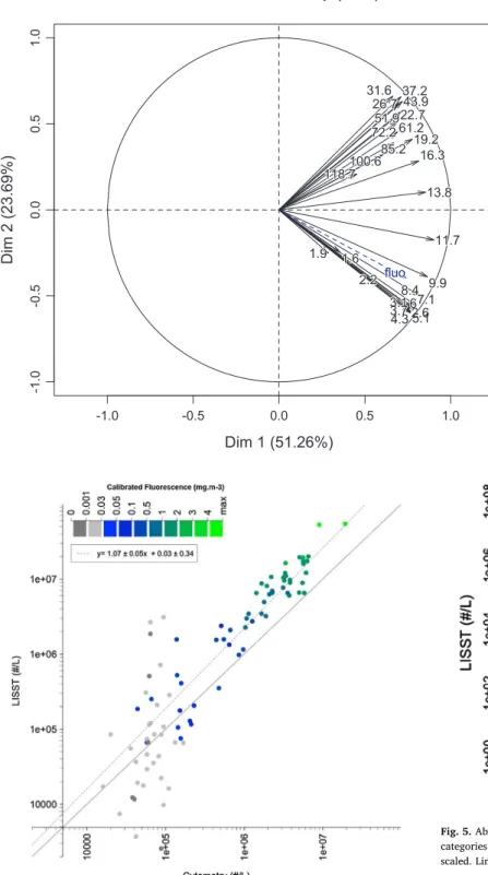
The PCA of VC (Fig. 3) showed that almost all size classes strongly co-varied with axis 1 which represented 51% of the variance. Axis 2 represented 24% of the variance and separated two groups of classes: a first group containing classes 2.1–10.8 µm with a negative correlation with axis 2 and a second group containing classes from 15.0 to 109.2 µm with a positive correlation. Classes 1.6, 1.9 and 118.7 µm were excluded from the groups due to their low loads with dimension 1.

These two groups were not correlated as illustrated by the angle∼90° between the two groups of vectors. The first group co-varied with fluorescence as shown by the PCA and Spearman correlations (rho al-ways > 0.74, p < 10−3).

Based on the grouping of classes obtained by PCA, instead of using the definition of the ‘nano’ size range 2–20 µm, we used particles with a size range between 2.1 µm and 10.8 µm to compare with nanophyto-plankton abundances determined by traditionalflow cytometry. From now on, we will refer to the 2–11 µm Particle Pool and the 15–109 µm Particle Pool for simplicity. The l 2–11 µm pool represented more than half of total VC and 79% of total particles in terms of abundance. The 15–109 µm pool represented 26% of total VC. Total VC (1.5–128.9 µm) ranged from 0.09 to 1.27 µL L−1in the upper 70 m and decreased to about 0.04 µL L−1below 70 m.

The Total Particle Volume was summed for sizes 1.25–109.2 µm, including thefirst size class in order to compare our results with other studies (noted hereinafter TPV1,25–109). It was on average 0.35 ± 0.18

µL L−1with a maximum of 0.86 µL L−1between 20 and 80 m depth. Below, at 125 m depth, TPV1,25–109dropped to 0.094 ± 0.082 µL L−1.

Considering the two particle pools 2–11 µm and 15–109 µm, on average TPV2–11was 0.30 ± 0.19 µL L−1above 70 m, and 0.18 ± 0.14 µL L−1

for depths above Zfluo=0.03. For particle pool 15–109 µm, TPV15–109was

equal to 0.13 ± 0.09 µL L−1 within the upper 70 m layer, and 0.10 ± 0.06 µL L−1 for depths above Zfluo=0.03. Below Zfluo=0.03,

TPV2–11 strongly decreased to 0.004 ± 0.003 µL L−1 and TPV15–109

dropped to 0.014 ± 0.016 µL L−1. These values did not take into ac-count depths deeper than 1000m to avoid the bottom nepheloid layer (Durrieu de Madron et al., 2017). Over the upper 150 m, the median size D50twas 54.1 µm and D50nanowas 14.7 µm. When only the upper

70 m were considered, D50tdecreased to 15.9 µm and D50nanoto 5.4

µm.

3.3. Estimation of the phytoplanktonic fraction within the 2–11 µm particle pool

For the nanophytoplankton size classes, there was a good correla-tion between particle abundances from LISST and nanophytoplankton abundances determined by traditionalflow cytometry (Spearman rho = 0.92, p < 10−3). LISST abundances were most of the time higher than traditionalflow cytometry. The scatter is also reduced for higher abundances.

The proportion between LISST and traditional flow cytometry abundance measurements was computed with the 56 samples above Zfluo = 0.03. Regardless offluorescence, the ratio LISST/traditional flow

cytometry was greater than 1 (median = 2.82).

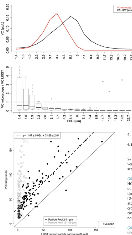
Nanodiatoms and nanoflagellates were counted by optical micro-scopy and abundances were compared with the LISST 2–11 µm abun-dance (Fig. 5). For both nanodiatoms and nanoflagellates, the spearman correlation was significant (respectively rho = 0.49, p = 0.013 and rho = 0.52, p = 0.008). However, LISST abundances were much higher than total nanophytoplankton counts (median about 6.76 times more). This ratio was closer to 1 when abundances increased.

3.4. Composition and size distribution of plankton cells

Two main dominant groups were identified by optical microscopy: nanoplanktonic diatoms and diverse nanoflagellates (respectively 18% and 78% on average abundance over the 32 samples). They were the dominant groups except at stations 88 and 89 (South) where small di-noflagellates were more numerous. Diatoms were dominated every-where by species Minidiscus trioculatus (on average 93%) with a max-imum abundance observed at station 84 with 19. 106_{cells L}−1 _and

representing 88% of total plankton counted. This centric diatom species is cylindrical with diameter from 2 to 5 µm (Throndsen et al., 2007). Nanoflagellates dominated the nanoplankton community in 20 out of 32 stations where they represent 90% of the total plankton counted by

optical microscopy. For many stations, this was the only taxon visible by optical microscopy. The maximum recorded concentration was 75·106_{cells L}−1_{at station 28.}

The PSD determined from optical microscopy (ImageJ processing) and LISST measurements both showed a particle volume maximum for

sizes between 3 and 6 µm (Fig. 6a). Median particle volume estimated from microscopy was smaller than that determined by the LISST (Fig. 6b).

3.5. Contribution of the small and large particle pools to POC

A good agreement between LISST derived particle carbon for Particle Pool 2–11 µm and POC was found (Fig. 7) at depths above Zfluo=0.03. The variation in LISST derived particle carbon was

essen-tially driven by the 2–11 µm Particle Pool. The LISST derived particle carbon of the 15–109 µm Particle Pool was not correlated with POC and was approximately constant throughout the water column (average 5.4 mgC m−3).

Fig. 3. PCA of VC table for size classes from 1.5 to 128.9 µm combining all measurements (numbers refer to the class centers). Only measure-ments above Zfluo=0.03were considered. The dotted blue arrow re-presents the supplementary variablefluorescence. The first axis con-tains 51.26% of total variance and the second, 23.69%. (For interpretation of the references to colour in this figure legend, the reader is referred to the web version of this article.)

Fig. 4. Abundances from the LISST Particle Pool 2–11 µm versus abundance from tra-ditionalflow cytometry (nanophytoplankton) for 108 samples gathered at stations 14, 16, 18–25 and 99. In dotted line, the linear model with formula between those variables for samples at depth above Zfluo=0.03. Solid line is equation y = x. Dots are colored from grey to blue then green according to their correspondingfluorescence. Axis are log scaled. The linearfit equation for non-transformed data is y = 3.05 ± 0.2 x – 2.69·105_{± 8.41·10}5_.

(For interpretation of the references to colour in thisfigure legend, the reader is referred to the web version of this article.)

Fig. 5. Abundances from the Particle Pool 2–11 µm vs abundances of the most abundant categories counted by optical microscopy, nanodiatoms and nanoflagellates. Axis are log scaled. Lines represent linear modelsfitting with these data (n = 27).

3.6. Typology of profiles for the 2–11 µm particle pool

The three clusters identified with the PAM method illustrate the gradient of profiles with high VC concentrated in the first 30 m (red) to profiles with lower VC diluted from 0 to 80 m (blue) (Fig. 8a). The intermediate cluster had a shape similar to the blue cluster but with higher VC. The horizontal distribution of clusters (Fig. 8B) showed a center region with high VC surrounded by a peripheral region of mixed intermediate and low VC, both on the northern and southern sides of the center region. The spot of intermediate VC in the south corre-sponded to an anticyclonic eddy (Fig. 8b and c).

4. Discussion

4.1. Particle pools seen by the LISST: Comparison with other studies Two particle pools were identified with LISST PSD, in the range 2–11 µm and 15–109 µm. These particle pools do not covary and their vertical distribution differ. We first review other studies reporting ob-servations of particle pools by LISST.

In February, during aflood event of the Rhône river,Many et al. (2016)identified several pools of particles with a 100 and LISST-HOLO over a meridional transect across the Gulf of Lions shelf. On the outer shelf, comparable to offshore waters sampled during DeWEX-2, three modes were identified on the PSD, centered around 10 µm (3–30µm), 100 µm (30–200 µm) and 400 µm. The 10 µm mode was attributed tofine silts, while the 100 µm mode was identified as mi-croflocs, themselves composed of fine grained particles from Rhone river. The potential contribution of phytoplankton to these pools was not quantified.

In the Cretean Sea (Eastern Mediterranean) Karageorgis et al. (2012)observed a PSD dominated by particles of size around 60–80 µm identified as microflocs. Spring TPV1,25–250 was generally 6–10 µL L−1in 0–15 m, and was < 1 µL L−1in deep water. Microflocs < 100 µm dominated TPV with D50 between 82 and 92 µm. Aggregates were generally in the 60–80 µm size range, some larger aggregates (100 µm) were fecal pellets. Our particulate pool 15–109 µm probably corre-sponds to the pool covering sizes 30–200 µm identified as microflocs by

Many et al. (2016)over the outer Gulf of Lions andKarageorgis et al. (2012)in the Cretean Sea. Its particle volume is higher in thefirst 70 m but it is still present at depth below 70 m (Fig. 2), for some profiles

down to 1000 m deep. This vertical distribution, extending far below the surface layer, suggests non-living particles in this pool (detritus, aggregates and/or terrigenous particles).

The 2–11 µm pool detected here was not shown inKarageorgis et al. (2012). In contrast,Barone et al. (2015)reported a similar particle pool of size between 3 and 10 µm in the oligotrophic Northern Pacific Subtropical gyre during summer. This pool dominated their VC (90% of 1.25–109.2 µm for depths 20–180 m) but no composition was available. The TPV1,25–109 ofBarone et al. (2015)was 0.076 ± 0.014 µL L−1for 20–80 m with a maximum of 0.16 µL L−1_{close to the mixed layer}

Fig. 6. (A) An example of PSD from optical microscopy and LISST at station 28 and (B) Boxplot of the ratio VC (microscopy)/VC (LISST) for the seven stations considered. ESD marks represent class centers.

Fig. 7. POC vs LISST derived particle carbon. Solid line: line y = x. Dotted line: linear model for the Particle Pool 2–11 µm. Spearman correlation test is significant p-value <

depth. In the same location but taking into account seasonal fluctua-tions, White et al. (2015)reported a TPV1,25–109 of 0.065 ± 0.033

µL L−1at 25 m and 0.032 ± 0.017 µL L−1at 125 m. Our data showed about 10 times higher particle volume for the same depth range and season.

ForBarone et al. (2015)andWhite et al. (2015), particles larger than 100 µm were below detection and thus not quantified. Conse-quently, they observed a Davg of 10.7–11 µm for 0–150 m and the 2–20 µm fraction dominated TPV. In our study, Davg is about 12.4 µm on average which confirms the dominance of the 2–11 µm particle pool in the full particle pool. The 15–109 µm particle pool made up of micro-flocs with probably sediment and/or riverine origin is thus peculiar to the Mediterranean basin. The location of Station ALOHA, remote from terrestrial influences and in the subtropical gyre, probably explains the absence of this pool.

4.2. Nature of particles seen by LISST

To better understand what is the type of the particles detected by the LISST, PSD data were compared with several discrete measure-ments.Table 2summarizes the characteristics of each method.

LISST derived particle carbon and POC strongly co-varied (Fig. 7).

Barone et al. (2015)also showed a strong co-variation of LISST derived

particle carbon and POC. Using VC from 1.25 to 109.2 µm,Barone et al. (2015)estimated that about 38% (according to theirFig. 7) of total particulate carbon was contributed by LISST derived particle carbon between 25 and 75 m depth. In our study, LISST derived particle carbon for the same size range and the 10-75m layer, represented on average 60% (CI95%: 0.53–0.67) of POC. Our figures are larger in magnitude and indicate the dominance of larger (2–11 µm) particle sizes in the total POC than forBarone et al. (2015). Considering the high correla-tion obtained, LISST derived particle carbon can be used as a proxy for POC in our dataset.

Moreover, the linear model computed on these data for the 2–11 µm particle pool showed a very close relation between total POC and LISST derived particle carbon for this size class Indeed, coefficients are sig-nificant with a slope close to 1 (Fig. 7). This means that POC variations are mostly driven by the abundance of particles between 2.1 and 10.8 µm. Additionally, the stoichiometry of the POM is peculiar (on average 42 ± 38:9 ± 6:1 for C:N:P molar ratio above Zfluo=0.03). The C:N ratio

(4.2 ± 1.9) is lower than Redfield ratio (6.6). This low C:N is typical of phytoplankton populations experiencing high growth rates (Goldman et al., 1979). This intense growth is also supported by high primary production estimates ranging from 85 to 9036 mgC/m2_{/d for the upper}

50 m (median 1444 mgC/m2/d, P Conan et al., unpublished data). Conversely, there is no correlation of POC with the 15–109 µm LISST Fig. 8. Clusters of the VC over the Particle Pool 2–11 µm from the LISST. Only thefirst 70 m of profiles were used. (A) Vertical profiles of the quantiles 25, 50 and 75 of the total VC for each cluster (B) Horizontal distribution of the three clusters (C) Boxplot of the VC over the Particle Pool 2–11 µm for each cluster.

derived particle carbon suggesting an inorganic nature as in

Karageorgis et al. (2012).

Compared to cytometry data, the 2–11 µm LISST particle pool co-varied strongly with nanophytoplankton counted by traditionalflow cytometry (Fig. 4; rho = 0.92). However, LISST abundances were about 3 times higher than those obtained by traditionalflow cytometry. First, this higher abundance from LISST is expected as living, non-living and inorganic particles are all counted, while theflow cytometry count is triggered by fluorescence induced in pigments present in phyto-plankton. Second, we suspect an underestimation by traditionalflow cytometry. Underestimation by traditionalflow cytometry is supported by the comparison of abundances obtained with continuousflow cy-tometry, which analyzes a larger volume (5 mL instead of 0.5 mL). Comparing measurements for the best-matching surface water samples (sampled at distance < 2.4 km), traditional and continuousflow cyto-metry results were strongly correlated (Rho = 0.9, n = 9), but con-tinuousflow cytometry counted on average 2.90 times more particles within the nanophytoplankton group (IC95%: 1.96–3.84) (data not shown). This underestimation was already observed (Thyssen et al., 2014) but its causes are not settled. Taking this underestimation of traditional flow cytometry into consideration, the abundance of the nanophytoplankton determined byflow cytometry is roughly equiva-lent to the LISST abundance for particle pool 2–11 µm. Since both in-struments gave similar results in particle counts, this suggests that the 2–11 µm pool is dominated by nanophytoplankton and that the LISST can be used successfully to monitor it.

Compared to optical microscopy observations in the range 1–15 µm, the average of particles detected by the LISST is larger than that esti-mated by microscopy (Fig. 6). This can be partly linked to the lugol fixation of samples (up to 10% decrease in diameter,Montagnes et al., 1994) but the LISST also assumes particle sphericity which could in-fluence its counting (Karp-Boss et al., 2007). The abundance estimated by optical microscopy is much smaller than the LISST abundance. Based on the good agreement between LISST and cytometry abundances (Fig. 4), we suspect an underestimation of abundance by optical mi-croscopy for this size range, possibly linked to the non-counting of aggregates containing cells. In terms of phytoplanktonic composition, microscopy analysis showed a large nanophytoplanktonic abundance with dominance of nanoflagellates and actively growing nanodiatoms dominated by Minidiscus trioculatus (numerous dividing cells). The size range of these diatoms (diameter of 1–5 µm when the cell is not in di-vision) is consistent with the LISST 2–11 µm peak.

The phytoplanktonic nature of the 2–11 µm pool is also supported by itsfluctuation with respect to the hour of the day. PSD were time averaged into 4h time bins. In the 0–30 m layer, we found a significant increase of particle volume from the morning to the afternoon (resp. 0.34 ± 0.22 µL L−1from 7 to 11 am and 0.62 ± 0.48 µL L−1from 3 to 11 pm, Kruskal-Wallis chi-squared = 33.04, p = 3.7 · 10−6). Mean size also increased from the morning to the afternoon (4.67–5.00 µm, Kruskal-Wallis chi-squared = 13.9, p = .016). This is consistent with phytoplankton cell cycle observations by cytometry in the Northwestern Mediterranean Sea (Dugenne et al., 2014; Thyssen et al., 2014). Daylight allows photosynthesis to occur, leading to an increase of cell size and total particle volume in the afternoon, while at night cells divide leading to smaller sizes in the morning (Vaulot and Chisholm, 1987).

4.3. Spatial distribution of the 2–11 µm particle pool

The three clusters of LISST VC profiles for the 2–11 µm particle pool illustrate three types of profiles, from low (blue), intermediate (green), to high (red) VC (Fig. 8). These three profile types are essentially

dis-tinguished by their integrated value of VC, and to a lesser extent by their shape. The increasing value of integrated VC from the blue to the red cluster is consistent with increasing POC, Chl-a and nanophyto-plankton abundance values as shown in Fig. 9. To understand the

Table 2 Main characteristics of the methods used to estimate nanophytoplankton abundances used in this study. Note that these characteristics are speci fi c to this study. For cytometry, the eff ective upper size limit is smaller than the theoretical one given. Method Sample type Size range (µm) Limited by Type of particles counted Volume analyzed per sample (mL) Known biases LISST Continuous (1 Hz), in situ 1.48 –128.9 Sensors sensitivity. Variable bin resolution. Contamination by out of range particles All 1.41 Eff ect of background measurement. Leakage eff ect, spherical shape assumption Traditional fl ow cytometry Discrete, from Niskin bottle, fi xed with glutaraldehyde and stored in liquid nitrogen 0.5 –100 Sensors sensitivity, tubing size, volume analyzed and abundances, software and hardware limits All above a given fl uorescence threshold 0.5 Underestimate nano and microplankton. Cell loss due to fi xation ( Marie et al., 2014 ) Continuous and automated scanning fl ow cytometry Discrete, sample from surface pumped seawater ∼ 0.5 –800 (width) Sensors sensitivity, tubing size volume analyzed and abundance, software and hardware limits All above a given fl uorescence threshold 5 Underestimate microplankton Optical microscopy Discrete, from Niskin bottle, fi xed with lugol 1– 1000: Optic resolution and volume of sedimented samples (note: for sizes < 5 identi fi cation is di ffi cult) All living particles 100 (diatoms) 1 (nano fl agellates) Underestimate nano fl agellate < 5µm, ignore cells in aggregates. Shrinking due to lugol (up to 10% ESD)

horizontal distribution of these three profile types, it is useful to con-sider the preceding winter period when deep convection was occurring over a large region centered on station 99 (SeeDonoso et al., 2017; Mayot et al., 2017andSeverin et al., 2017). This intense process cre-ated two well defined zones: the Deep Convection Zone (DCZ) with homogeneous vertical profiles, low phytoplankton and high nutrient concentrations, and the peripheral zone with various degrees of stra-tification and phytoplankton abundance. In spring, the horizontal cir-culation and turbulent restratification has only weakly modified the winter distribution. The DCZ stratified later than the peripheral zone, which led to a later but stronger phytoplankton bloom (Mayot et al., 2017).

The cluster with high VC (red) is present in the former convection region and shows surface maximum VC and Chl-a, typical of a recent bloom. The intermediate cluster (green) is spread in the peripheral region of the convection (Fig. 8b and c). The low VC cluster (blue) is scattered North and South of the convection region, except East of Baleares, where there is a contiguous region of low VC. In the vertical, the VC profile shape generally resembles the fluorescence profile (see

Fig. 2) except near the surface, probably due to non-photochemical quenching. When a deep Chl-a maximum was present, its depth cor-responded to a local maximum of VC but weaker in amplitude, possibly

indicating photoacclimation. 4.4. Limits of our analysis

The conditions of the cruise were favorable for use of the LISST to quantify the phytoplankton pool: open ocean waters, actively growing cells and high dominance of a few cell types approximately spherical in shape. Other datasets must be gathered to test whether our results can be easily replicated elsewhere.

In order to use LISST data, a background (clear water) scattering value has to be subtracted before the inversion step to estimate the particle volume. This background value is estimated by either clear water (usually 0.2 µmfiltered) on deck or in situ clear water. Here, as

Barone et al. (2015), we chose to use the minimum of in situ scattering between 200 and 1000m for each profile. Since this layer has low and rather constant POC (10–50 mgC m−3_{), we argue that it can be}

con-sidered as a stable reference across stations, with the change of back-ground being only due tofluctuations in the instrument's optics. Using a single background value applied to all the profiles led to a dataset with a larger variance across profiles and was therefore abandoned. The high VC and variability at classes 31 and 32 (> 180 µm) possibly con-taminated classes smaller than 130 µm. The origin of these high values Fig. 9. Boxplot of environmental variables (Mixed layer depth (Zmld), Zfluo=0.03, Cytometry abundance, Fluorescence, POC, Chl-a, POC:PON) according to clusters defined on LISST VC

profiles. Same colors asFig. 8. For depth-resolved variables, only depths 0–70 m were used. For cytometry, note that only 11 eleven stations were available. Clusters with same letters are not significantly different from each other according to a Kruskal-Wallis test followed by a Nemenyi post-hoc test.

and variability may lie in the suboptimal vertical positioning of the LISST-Deep on the rosette. Although we cannot accurately estimate the extent of this contamination, observations in controlled laboratory ex-periments showed a significant contamination of VC as far as 8 classes away from the actual size class of particles present in the sample (leakage effect,Agrawal and Pottsmith, 2000). We observed that high VC values at classes 31 and 32 led to reduced VC for classes down to 30µm. Therefore, the VC values for the 15–109 µm particle pool may be underestimated. Mounting the LISST horizontally below the rosette and using a slower cable velocity, which would produce more data per meter, could probably minimize the noise observed in classes 31 and 32.

5. Conclusion

As demonstrated by the combination of laser diffraction (LISST), flow cytometry, and optical microscopy data, the 2013 spring bloom in the Gulf of Lions was characterized by a dominance of nanophyto-plankton with mean size 5 µm, mostly represented by nanoflagellates and nanodiatoms (Minidiscus trioculatus). This nanophytoplankton dominance, observed byflow cytometry and identified by microscopy, was clearly distinguished in the LISST signal by a large peak between 2.1 and 10.8 µm. While cytometry and microscopy allows for the de-termination of bloom composition for a limited number of depths and stations, in situ deployment of LISST provides high-resolution, depth-resolved distributions and sizes of key particle pools over an extended area thanks to its high sampling frequency. To further take advantage of these three techniques to characterize phytoplankton, dedicated la-boratory experiments must be undertaken. As a perspective, since LISST is mostly restricted to the size class < 200 µm (nano- and micro-plankton and particles), we believe it would be very promising to combine the LISST with the LOPC and the Underwater Vision Profiler in order to build a continuous particle size distribution covering pico-phytoplankton to zooplankton, along with identification of larger par-ticles (Picheral et al., 2010). This will help to characterize ecosystem productivity, the transfer of energy to upper trophic levels (Espinasse et al., 2014) and vertical matter export from the surface to the deep ocean (Guidi et al., 2008).

Acknowledgements

We acknowledge sponsorship from WP2 MISTRALS-MERMEX pro-gram. This study is a contribution to the international SOLAS, IMBER and LOICZ program, supported by Pôle Mer Méditerranée. We thank Véronique Cornet-Barthaux for help with microscopy, Alain de Verneil for english proofreading, as well as the captain and crew of R/V Le Suroît. R Leroux was funded by MERMEX-IPP. All data used are available through http://mistrals.sedoo.fr/MERMeX/. The two re-viewers are thanked for their constructive comments that helped im-proving the manuscript.

References

Agrawal, Y.C., Pottsmith, H.C., 2000. Instruments for particle size and settling velocity observations in sediment transport. Mar. Geol. 168 (1), 89–114.

Andrews, S.W., Nover, D.M., Reuter, J.E., Schladow, S.G., 2011. Limitations of laser diffraction for measuring fine particles in oligotrophic systems: pitfalls and potential solutions. Water Resour. Res. 47 (5).

Anglès, S., Jordi, A., Garcés, E., Masó, M., Basterretxea, G., 2008. High-resolution spatio-temporal distribution of a coastal phytoplankton bloom using laser in situ scattering and transmissometry (LISST). Harmful Algae 7 (6), 808–816.

Barone, B., Bidigare, R.R., Church, M.J., Karl, D.M., Letelier, R.M., White, A.E., 2015. Particle distributions and dynamics in the euphotic zone of the North Pacific Subtropical Gyre. J. Geophys. Res.: Oceans 120 (5), 3229–3247.

Caliński, T., Harabasz, J., 1974. A dendrite method for cluster analysis. Commun. Stat.-Theor. Methods 3 (1), 1–27.

Claustre, H., Hooker, S., Van Heukelen, L., Berthon, J.-F., Barlow, R., Ras, J., Sessions, H., Targa, C., Thomas, C.S., Van Der Linde, D., Marty, J.C., 2004. An intercomparison of HPLC Phytoplankton pigment methods using in situ samples: application to remote

sensing and database activities. Mar. Chem. 85, 41–61.

Conan, P., 2013. DEWEX-MERMEX 2013 LEG2 cruise. RV Le Suroît.http://dx.doi.org/10. 17600/13020030.

De Boyer Montegut, C., Madec, G., Fischer, A.S., Lazar, A., Iudicone, D., 2004. Mixed layer depth over the global ocean: an examination of profile data and a profile-based climatology. J. Geophys. Res.– Oceans.http://dx.doi.org/10.1029/2004JC002378. Donoso, K., Carlotti, F., Pagano, M., Hunt, B., Escribano, R., Berline, L., 2017.

Zooplankton community response to the winter 2013 deep convection process in the NW Mediterranean Sea. J. Geophys. Res. Oceans.http://dx.doi.org/10.1002/ 2016JC012176.

Dugenne, M., Thyssen, M., Nerini, D., Mante, C., Poggiale, J.-C., Garcia, N., Garcia, F., Grégori, G.J., 2014. Consequence of a sudden wind event on the dynamics of a coastal phytoplankton community: an insight into specific population growth rates using a single cell high frequency approach. Front. Microbiol. 5, 485.http://dx.doi.org/10. 3389/fmicb.2014.004.

Durrieu de Madron et al., 2017. Deep sediment resuspension and thick nepheloid layer generation by open-ocean convection. J. Geophys. Res.– Oceans.http://dx.doi.org/ 10.1002/2016JC012062.

Espinasse, B., Carlotti, F., Zhou, M., Devenon, J.L., 2014. Defining zooplankton habitats in the Gulf of Lion (NW Mediterranean Sea) using size structure and environmental conditions. Mar. Ecol. Prog. Ser. 506, 31–46.

Font-Muñoz, J.S., Jordi, A., Anglès, S., Basterretxea, G., 2015. Estimation of phyto-plankton size structure in coastal waters using simultaneous laser diffraction and fluorescence measurements. J. Plankton Research, fbv041.

Goldman, J.C., MacCarthy, J.J., Peavey, D.G., 1979. Growth rate influence on the che-mical composition of phytoplankton in oceanic waters. Nature 279, 210–215.

Grégori, G., Colosimo, A., Denis, M., 2001. Phytoplankton group dynamics in the Bay of Marseilles during a 2-year survey based on analyticalflow cytometry. Cytometry 44 (3), 247–256.

Guidi, L., Gorsky, G., Claustre, H., Miquel, J.-C., Picheral, M., Stemmann, L., 2008. Distribution andfluxes of aggregates > 100 mu m in the upper kilometer of the South-Eastern Pacific. Biogeosciences 5, 1361–1372.

Herman, A.W., Beanlands, B., Phillips, E.F., 2004. The next generation of optical plankton counter: the laser-OPC. J. Plankton Res. 26 (10), 1135–1145.

Karageorgis, A.P., Georgopoulos, D., Kanellopoulos, T.D., Mikkelsen, O.A., Pagou, K., Kontoyiannis, H., Kontoyianni, A., Anagnostou, C., 2012. Spatial and seasonal variability of particulate matter optical and size properties in the eastern medi-terranean sea. J. Marine Syst. 105, 123–134.

Karp-Boss, L., Azevedo, L., Boss, E., 2007. LISST-100 measurements of phytoplankton size distribution: evaluation of the effects of cell shape. Limnol. Oceanogr. Methods 5, 396–406.

Kostadinov, T.S., Siegel, D.A., Maritorena, S., Guillocheau, N., 2012. Optical assessment of particle size and composition in the Santa Barbara Channel, California. Appl. Opt. 51 (16), 3171–3189.

Many, G., Bourrin, F., de Madron, X.D., Pairaud, I., Gangloff, A., Doxaran, D., et al., 2016. Particle assemblage characterization in the Rhone river ROFI. J. Mar. Syst. 157, 39–41.

Marie, D., Rigaut-Jalabert, F., Vaulot, D., 2014. An improved protocol forflow cytometry analysis of phytoplankton cultures and natural samples. Cytometry Part A 85 (11), 962–968.

Mayot, N., D'Ortenzio, F., Ribera d'Alcalà, M., Lavigne, H., Claustre, H., 2016. Interannual variability of the Mediterranean trophic regimes from ocean color satellites. Biogeosciences 13 (6), 1901–1917.

Mayot, N., D'Ortenzio, F., Taillandier, V., Prieur, L., Pasqueron de Fommervault, O., Claustre, H., Ellipsis, Conan, P., 2017. Physical and biogeochemical controls of the phytoplankton blooms in North-Western Mediterranean Sea: a multiplatform ap-proach over a complete annual cycle (2012–2013 DEWEX experiment). J. Geophys. Res.: Oceans.http://dx.doi.org/10.1002/2016JC012052.

Menden-Deuer, S., Lessard, E.J., 2000. Carbon to volume relationships for dinoflagellates, diatoms, and other protest plankton. Limnol. Oceanogr. 45 (3), 569–579.

Mikkelsen, O.A., Milligan, T.G., Hill, P.S., Chant, R.J., Jago, C.F., Jones, S.E., et al., 2008. The influence of schlieren on in situ optical measurements used for particle char-acterization. Limnol. Oceanogr. Methods 6, 133–143.

Montagnes, D.J., Berges, J.A., Harrison, P.J., Taylor, F., 1994. Estimating carbon, ni-trogen, protein, and chlorophyll a from volume in marine phytoplankton. Limnol. Oceanogr. 39 (5), 1044–1060.

Peters, R.H., 1983. The ecological implications of body size. Cambridge Studies in Ecology 1576 (2), 1–325.

Picheral, M., Guidi, L., Stemmann, L., Karl, D.M., Iddaoud, G., Gorsky, G., 2010. The Underwater Vision Profiler 5: an advanced instrument for high spatial resolution studies of particle size spectra and zooplankton. Limnol. Oceanogr.-Methods 8, 462–473.

Pujo-Pay, M., Raimbault, P., 1994. Improvement of the wet-oxidation procedure for si-multaneous determination of particulate organic nitrogen and phosphorus collected onfilters. Mar. Ecol. Prog. Ser. 203–207.

Reynolds, A., Richards, G., de la Iglesia, B., Rayward-Smith, V., 1992. Clustering rules: a comparison of partitioning and hierarchical clustering algorithms. J. Math. Model. Algorithms 5, 475–504.

Rienecker, E., Ryan, J., Blum, M., Dietz, C., Coletti, L., Marin III, R., Bissett, W.P., 2008. Mapping phytoplankton in situ using a laser-scattering sensor. Limnol. Oceanogr. Methods 6, 153–161.

Schneider, C.A., Rasband, W.S., Eliceiri, K.W., 2012. NIH Image to ImageJ: 25 years of image analysis. Nat. Methods 9 (7), 671–675.

Schöniger, 1952. Über eine Modifikation der Mikrostickstoffbestimmung nach Dumas-Pregl. Microchim. Acta 39 (3), 229–233.

Evaluation of laser in situ scattering instrument for measuring concentration of phytoplankton, purple sulfur bacteria, and suspended inorganic sediments in lakes. J. Environ. Eng. 127 (11), 1023–1030.

Severin, T., Kessouri, F., Rembauville, M., Sánchez-Pérez, E.D., Oriol, L., Caparros, J., Ellipsis & Mayot, N., 2017. Open-ocean convection process: a driver of the winter nutrient supply and the spring phytoplankton distribution in the Northwestern Mediterranean Sea. J. Geophys. Res.: Oceans.http://dx.doi.org/10.1002/ 2016JC012664.

Strickland, J.D.H., 1965. Phytoplankton and marine primary production. Annu. Rev. Microbiol. 19, 127–162.

Throndsen, J., Hasle, G.R., Tangen, K., 2007. Phytoplankton of Norwegian Coastal Waters. Almater Vorlag As, Oslo, pp. 343p.

Thyssen, M., Gregori, G.J., Grisoni, J.-M., Pedrotti, M.-L., Mousseau, L., Denis, M.J., 2014. Onset of the spring bloom in the northwestern Mediterranean Sea: influence of en-vironmental pulse events on the in situ hourly-scale dynamics of the phytoplankton community structure. Front. Microbiol. 5.

Vaulot, D., Chisholm, S.W., 1987. A simple model of the growth of phytoplankton po-pulations in light/dark cycles. J. Plankton Res. 9 (2), 345–366.

Veldhuis, M.J., Kraay, G.W., 2000. Application offlow cytometry in marine phyto-plankton research: current applications and future perspectives. Scientia Marina 64 (2), 121–134.

Vidussi, F., Claustre, H., Bustillos-Guzman, J., Cailliau, C., Marty, J.C., 1996. Determination of chlorophylls and carotenoids of marine phytoplankton: separation of chlorophyll a from divinyl-chlorophyll a and zeaxanthin from lutein. J. Plankton Res. 18, 2377–2382.

White, A.E., Letelier, R.M., Whitmire, A.L., Barone, B., Bidigare, R.R., Church, M.J., Karl, D.M., 2015. Phenology of particle size distributions and primary productivity in the North Pacific subtropical gyre (Station ALOHA). J. Geophys. Res.: Oceans 120 (11), 7381–7399.

Yentsch, C.M., Horan, P.K., Muirhead, K., Dortch, Q., Haugen, E., Legendre, L., et al., 1983. Flow cytometry and cell sorting: a technique for analysis and sorting of aquatic particles. Limnol. Oceanogr. 28 (6), 1275–1280.