Advanced controls for floating wind turbines

Advanced Controls for Floating Wind Turbines

Carlos Casanovas

Lic. Industrial Engineering

Universitat Politecnica de Catalunya (UPC-ETSEIB) 2006

SUBMITTED TO THE DEPARTMENT OF MECHANICAL ENGINEERING AND NAVAL

ARCHITECTURE IN PARTIAL FULFILLMENT OF THE REQUIREMENTS FOR THE DEGREE OF MASTER OF SCIENCE IN MECHANICAL ENGINEERING

AT THE

MASSACHUSETTS INSTITUTE OF TECHNOLOGY Ui E

JUNE 2014

AU6

15 2014

@2014 Massachusetts Institute of Tec Iology. All rights reserved.

Signature redacted

Signature of Author:

Department of Mechanical Engineering and Naval Architecture

--

/-

Signature redacted

Certified by:

Accepted by:.

Professor Paul D. Sclavounos Professor of Mechanical Engineering and Naval Architecture

Signature

redacted'

"perviso

Professor David E. Hardt Professor of Mechanical Engineering and Naval Architecture

Advanced Controls for Floating Wind Turbines

Carlos Casanovas

Submitted to the Department of Mechanical Engineering on May 20, 2014 in Partial Fulfillment of the Requirements for the Degree of Master of Science in

Mechanical Engineering

ABSTRACT

Floating Offshore Wind Turbines (FOWT) is a technology that stands to spearhead the rapid growth of the offshore wind energy sector and allow the exploration of vast high quality wind resources over coastal and offshore areas with intermediate and large water depths. This generates the need for a new generation of Wind Turbine control systems that take into account the added complexity of the dynamics and wave-induced motions of the specific floater. The present work presents a simulation study of advanced controls for Tension Leg Platform (TLP) FOWT that attempts to enhance the power output of the Wind Turbine by conversion of the surge kinetic energy of the TLP into wind energy. The public access data of the NREL 5MW offshore wind turbine have been used to perform the study.

After establishing a theoretical upper bound for the possible wave energy extraction using frequency-domain methods, a time-domain state-space dynamic model of the FOWT with coupled dynamics of platform surge motion and turbine rotation has been developed that includes both a simplified model of the turbine aerodynamics and the floater surge hydrodynamics. This simulation model has then been used to implement advanced controls that maximize energy extraction by the Wind Turbine in the below rated power region. The proposed controllers are variations of a Linear-Quadratic Regulator (LQR), considering both a steady-state case and a non-stationary, finite horizon LQR case. The latter requires wave-elevation forecasting to be implemented and therefore two different forecasting algorithms have also been developed according to existing literature.

While the wave-induced annual energy yield enhancement of the studied FOWT in the two considered locations is small (around 0.02% the baseline annual energy yield of the studied turbine in the two locations) the study is not exhaustive and other FOWT topologies might achieve better results. The present results clearly indicate, however, that the existing correlation between strong wind and waves makes FOWTs a sub-optimal choice as energy

ACKNOWLEDGEMENTS

I would first like to thank Prof. Sclavounos for giving me a chance to work in his lab and for

the continuous research guidance over the last two years. It has been a fantastic learning experience in all fronts. My gratitude in this regard also goes to all my lab mates, and especially to Godine Chan, who has been there for me on good times and bad. Best of luck to all of you.

Also my sincerest thanks to the Alstom Wind team, which has supported my research here and provided help and insightful research feedback along the way. In particular I would like to thank Dhiraj Arora for the massive amount of useful feedback along the way, Jose-Luis Roman and Jordi Puigcorbe for supporting my desire to come to MIT and making it possible, to Elena Menendez for all her useful advice, and the U.S. Department of Energy which has funded this research through grant no. DE-EE0005494.

Finally I would like to thank my family and friends for their continuous support and faith in me. I would not be anywhere near where I am now if it was not for them.

Contents

1 . In tro d u c tio n ... 1 0

2. System description and modeling... 12

2.1 General model of the TLP wind turbine ... 12

2.2 Hydrodynamic model of the buoy ... 14

2 .3 A ero d y n am ic m o d el...1 8 3. Frequency domain approach ... 20

3.1 Seastate and wave spectrum ... 20

3.2 W ave energy extraction in frequency domain ... 20

3.3 Wave power extraction potential for NREL 5 MW turbine...24

4. Control implementation in time domain... 26

4 .1 M o d el lin ea rizatio n ... 2 6 4.2 Time domain implementations of the wave exciting force... 28

4.3 The baseline NREL controller ... 29

4.4 LQR and the cost function...30

4 .5 S tead y -state L Q R ... 3 2 4 .6 F in ite-h o rizo n L Q R ... 3 4 4 .7 O v erlaid L Q R co n trol ... 3 5 5. Time domain control results... 36

5.1 Sensitivity analysis of finite-horizon LQR parameters ... 36

5.2 Results with different control options... 38

6. Annual energy yield enhancement ... 42

7. W ave elevation forecasting...44

7.1 Relation between wave exciting force and wave elevation ... 44

7.2 Autoregressive (AR) forecasting... 46

7 .2 .1 A R m o d el th eo ry ... 4 6 7.2.2 AR model performance and parameter sensitivity... 48

7.3 .1 E SP R IT m eth o d th eo ry ... 51 7.3.2 ESPRIT method performance and parameter sensitivity ... 53 8 . C o n clu sio n s ... 6 2 9 . R e fe re n ce s ... 6 4

Appendix I: Adaptation of NREL turbine to a new TLP ... 66

Transition piece and arms adaptation...66

F lo ater a d a p tatio n ... 6 7

Tower and turbine adaptation ... 67

Appendix II: Stochastic linearization of viscous damping ... 68

g p t S Hs A Tm R L M A((o) A. B (o) Bw(o) BT CD C D K(t) K(s) fM(t) U X(t) X(W) fe(t) h FT P

NOMENCLATURE

Wave elevation spectrum Significant wave height Wave amplitude

Standard deviation Mean wave period Buoy Radius Buoy Draft

System mass coefficient in surge Freq. dependent added mass coef. Added mass coef. for infinite freq. Freq. dep. hydrodyn. damping Linearized total hydrodyn. damping Equivalent turbine damping Drag coefficient

Restoring coefficient (stiffness) Viscous damping coefficient Retardation function

Laplace trans. of retardation function Hydrodynamic forces related to memory effects

Time domain surge displacement Freq. domain surge displacement Freq. domain surge velocity

Time domain wave excitation forces Freq. domain wave excitation forces Normalized wave excitation

Impulse response of surge exc. force Wind thrust force

Power

p coef. of numerator polynomial of a transfer function

q Coef. of denominator polynomial of a transfer function

x System state

u System input [X] State vector

[U] Input vector

As, Bs, Cs, Ds State-space matrices for the mechanical system dynamics

V Wind speed

V. Far-field wind speed (upstream)

VR Wind speed at the rotor a Induction factor

A Tip-speed ratio J Control objective

RR Rotor radius

SR Swept rotor surface I Inertia

Cp Turbine power coefficient CT Turbine thrust coefficient

TAero Aerodynamic torque on rotor

TGen Electrical torque on generator

T1 Gearbox ratio

fl Rotor rotational speed

'M Rotor speed fluctuation around equilibrium position

0 Rotor collective pitch angle

$ Pitch angle fluctuation around equilibrium position

Note: despite the apparent conflicts for u, U, x, X, A, their meaning can always be easily determined from context

1. Introduction

The rapid expansion of the wind energy industry over the past 40 years, initially spurred by the 1973 oil crisis, is now moving offshore with the promise of stronger, steadier oceanic winds and the limitations of further onshore wind farm developments in areas where wind energy penetration is already high, such as Germany or Denmark. The first commercial offshore wind farms, erected in the 1990s, are located in very shallow waters in the North Sea, facilitating the use of fixed monopile foundations. The shallow waters of the North Sea are, however, more an exception than the norm, and fixed foundations become very expensive as water depth increases. For this reason there is an interest in the development of floating offshore wind turbines (FOWTs), and there are already a number of prototypes in the water that are experimenting with floater designs, most of them drawing from the extensive experience of the Oil & Gas industry with floating offshore rigs, as shown in figure

1.1.

Figure 1.1 - Floating wind turbine concepts adopted from the Oil & Gas industry. A spar buoy (left), a TLP (middle) and a semi-submersible (right). Image courtesy of the National Renewable Energy Laboratory (NREL)

While most of the underlying technology for the turbine itself (blades, tower, generator, etc) is common between onshore, fixed foundation offshore and floating offshore turbines, the latter have an added layer of complexity due to the dynamics of the floater and the ocean environment. This is particularly relevant in the area of turbine control systems, with existing control algorithms designed for fixed foundation turbines not being applicable for floating designs. Large displacements of the structure generate complex interactions with the rotational degree of freedom (DoF) and the aerodynamics of the turbine that need to be taken into account explicitly to achieve good turbine performance and avoid system instability.

The present work focuses on the specific case of a Tension Leg Platform (TLP) foundation, which has raised a lot of interest due to its relatively low weight and the stability it provides to the turbine, which is almost restricted to only move in surge and sway. A simple but well grounded state-space dynamic model of the TLP FOWT, including coupled dynamics of platform surge and the rotational DoF has been built in Matlab to study the potential absorption of ocean wave kinetic energy hitting the substructure by the wind turbine generator, without adding any new physical device specifically built for wave energy absorption. This would lead to some degree of energy yield enhancement when the turbine is operating below its rated power. The model has then been used to develop advanced controls that maximize the wave energy extraction capacity of the system. This involves the creation of a state-space description of the hydrodynamic and aerodynamic properties of the turbine and floater, the implementation of algorithms for wave elevation forecasting that would be necessary, and the creation of of the advanced control algorithms themselves, which are variations of the well known Linear Quadratic Regulator (LQR) adapted to the specific problem. While the actual wave energy extraction potential of the studied turbine have been found to be low compared to its baseline annual power production, the developed models are a good example of how to approach the complexity of coupled wave and wind dynamics on FOWTs, and the tools developed over the course of this work can be readily applied to other control problems for similar structures such as load mitigation and system stabilization.

2. System description and modeling

2.1 General model of the TLP wind turbine

The base system referenced throughout this report is based on the NREL 5 MW wind turbine, as described by NREL [1]. A tension leg platform (TLP) for this turbine has been developed for this work, adapting the design proposed by Garrad-Hassan [2]. Refer to Appendix I for a detailed description of this adaptation.

TLPs are characterized by a high heave and pitch stiffness, which makes an uncoupled modeling of the surge and sway dynamics possible. Considering the surge direction to be aligned with the WTG rotation axis (the direction of the wind), the surge equation of motion (EOM), which is built upon the Cummins equation, is the following:

(M+

A,

+ K(t -r)-dr+D +C

=

X(t)+Fr (t)

0

where

M System mass (platform + turbine)

A. Hydrodynamic added mass coefficient in surge for infinite frequency

K(t) Retardation function, related to hydrodynamic memory effects

C System restoring coefficient in surge

D System linearized viscous damping coefficient in surge S(t) Surge displacement

X

(t)

FT (t) Time dependent aerodynamic thrust force, from the WTG

The values for stiffness C and mass M are obtained by implementing the model in the Laboratory of Ship and Platform Flow (LSPF) existing frequency domain codes, but can be computed analytically by hand calculations in the case of the TLP given their relatively simple mooring line layout. A model for the retardation function K is described in section 2.2 leading to a state-space description of the hydrodynamic memory effects. The linearized value for the viscous damping coefficient is obtained through stochastic linearization, as described in Appendix II.

Rotational dynamics of the wind turbine have been simplified to a first order model, since rotor position is unimportant. Only its rotational velocity will matter for the problem being considered. The drive train is considered to be rigid, which is an adequate hypothesis considering the very low frequency dynamics of the wave phenomena under study. The rotation EOM is therefore:

dt

T

rotational speed of the rotor

inertia of the rotor plus generator, reduced to the low speed shaft aerodynamic torque on the rotor

electrical torque in the generator gearbox ratio

Rotor and generator Inertia, as well as gearbox ratio, are taken from the NREL 5 MW turbine data.

Regarding the controller, the documentation for the NREL 5 MW turbine [1] includes a thorough description of the control system, which operates on 3 main control regions and 2 transition regions. 50,000 40,000 E 30,000 0 20,000 C 10,000 0 400 600 800 Generator Speed, rpm 1,000 1,200 1,400

Fig. 2.1: Torque vs Speed response of the NREL torque controller [1]

Regions 2 and 3 are the main power-generating regions, with 2 being below rated power and 3 being above-rated power. Wave energy capture is restricted to region 2, since the turbine is already operating at full power in region 3 and it is not possible to absorb any additional energy from the waves at that point. The focus of this project is therefore in region 2. Region 1 1% 2 2/% 3 - Optimal - Variable-Speed Controller U h II 0 200

2.2 Hydrodynamic model of the buoy

The proposed TLP design is based on a cylindrical buoy of radius 4.75 m and draft 30 m, in

100 m water depth. Such a buoy has been implemented in WAMIT to obtain frequency

dependent added mass A(w), potential damping B(o), and complex exciting force X(W).

Due to the complexity of dealing with the convolution integral in the surge EOM, the methodology described by Perez-Fossen [3] has been used to fit the convolution integral in the Laplace domain, from which it can be transformed into a state-space model so that it can easily be implemented in time-domain simulations. Considering this convolution term, which describes a force related to fluid memory effects fM(t):

fK (t -r) -.edz- =

(t )

0

The convolution integral becomes simple products in the Laplace domain:

I {K(t-r)-dr

=K(s)-U(s)=F(s)

0

Now using the Ogilvie relationships (1964)

A(w)= AD- K(t)sin(wr)dr

B(w)= K(t)cos(wr)dr

combined with the Euler formulas for complex exponentials, the following expression can be obtained:

K

(jo)=

B(w)+

jw[A

(w)-

_A

This equation provides a direct formula for the frequency dependent transfer function K between surge velocity and the force related to memory effects FM which can be calculated for any given frequency using data from WAMIT or similar codes and even analytically for the cylinder case. Taking into account that the convolution integral describing fm can be related to a high-order ODE it can be seen that the Laplace transform of the retardation function acts as the transfer function between the frequency domain force FM and surge velocity U, which can be written as the quotient of polynomials P and

Q:

Fm (s) ps' + ps

_.

U(s) s" +

q

+

The challenge of fitting the known properties of K in the frequency domain is addressed by Perez and Fossen [3], who provide a clear methodology and an implementation using MATLAB. A number of constraints can be placed into this transfer function due to the characteristics of fluid memory models that are reflected in the retardation function. These constraints are summarized in

Table 2.1:

Property Implications Comments

K(s) has zeros at s = 0 Low frequency asymptotic

1imO K

(jc)=

po =0. zero for o =0

High frequency asymptotic K(s) is strictly proper. value of K(s). Denominator deg(Q) > deg (P) has to grow faster with

frequency. 2

limt

J

(a)do

Laplace transform for K(t)

s-- s--

Q(s)

Bounded-input bounded- Final-time value of K(t).

lim,_0

the model zero at infinite time.

Passivity is a property Mapping of

I-+>fm

nature of K(t).

The iterative approach provided by Perez and Fossen can be summarized in the following algorithm [3]:

1. Calculate the frequency response K(jw) for an adequate number (i) of frequencies (Wi)

2. In order to avoid numerical problems due to the numerator coefficients being much larger than the denominator, scale the vector dividing it by the maximum value obtained for K for all wi

K'(jco)= a -K(jo,)

aD

1

max K (jo)

3. Select the order of the approximationn

deg(Q(jw,0)).

n=2.

4. Estimate the parameters

0* = arg min

P'(jio,,0)

jw,

Q(io,,0)

Where P'(s)= P(s) _{is used, and it can be shown that it has no roots on the imaginary axis} S

of the complex plane and has a degree deg(P') = n -2

(To solve this non-linear complex curve fitting a Gauss-Newton algorithm can be used, or else a linear approximation)

5. Check stability. Computing the roots A n..., of Q(io,0*) and change the sign of

the real part of the roots that are found to have positive real part. This has to be done unless stability has been enforced as a constraint in the optimization algorithm in the previous step.

6. Construct the desired transfer function:

I s -P'( s, 0*

K(s)=---

(

a Q(s, 0*)

7. _{Estimate the added mass and damping based on the approximation that has been}

obtained, using:

A(CO)= Im

o'K (io)+

A

(c)= Re{K (Ico)

Compare this result with the original added mass and WAMIT or analytical calculations. Repeat steps 3 to approximation until an acceptable fit is obtained.

damping coefficients given by

7 increasing the order of the

This implementation has been adapted for this project, and an order 4 model is found to be enough to adequately describe the added mass and damping of the system throughout the required range of frequencies. Figure 2.2 shows the added mass and potential damping comparison between the original WAMIT dataset for the buoy and the output of the fitted model in frequencies from 0 to 5 rad/s.

x 105 Potential Damping in Surge 10

5 0

-5

2.2

0 Original WAMIT dataset S... ... Identification of order 4

0.5 1 1.5 2 2.5 3 3.5 4 4.5

Frequency [rad/s]

X 10 Added Mass in Surge

0.5 1 1.5 2 2.5

Frequency [rad/s]

3 3.5 4 4.5

Fig. 2.2: Added mass and potential damping fit through a fourth order model

Once the K transfer function polynomial coefficients have been fitted, it is straightforward to transform K into a state-space model with a number of parameters that is equal to the order of the system, in this case 4. Using the phase-variable canonical form:

T E 0 2 -) I&) 1.8 1.8 1.4 5

'

0 Original WAMIT dataset

... Identification of order 4 ... . ... ... ... ... I. ... - - - - - - - - - - - - - - -- - - -. -. -. -. -. -.-.-. . . . . . . . . --

-x 0 0 0

-q

-q

F

_"

_1]rX2

Li

These internal states x, to X4 represent the memory effects, with x₄ being already the

desired output. It can be shown that the system is fully observable, and therefore these states can be used in a full-state feedback control loop.

2.3 Aerodynamic model

A simplified aerodynamic model is considered for evaluation of the aerodynamic thrust FT

and torque TAero using the definitions of power coefficient Cp and thrust coefficient CT [4]:

(

The main limitation of this model is that it assumes steady-state conditions, assumption that will no longer hold considering the dynamic surge motion. However the surge velocity and specially the surge acceleration are small, due to the very low frequencies being considered, so a quasi-static approach seems still good enough at this stage.

The Cp and CT surfaces for the NREL 5 MW turbine were calculated using the code WTPerf v3.00 by Rannam Chaaban from Universtat Siegen (Germany), who has kindly authorized its use for this project. The available dataset has been implemented as a cubic spline surface in Matlab, in order to obtain the necessary partial derivatives.

PA

SR

RRQ

Thrust Coeffcient Ct 10, 5 n Pow 2 0 2 -0 -5 -0 0 ₀ 5 10 1i 20 25 30 5

Fig 2.3: The NREL 5MW Cp and CT surfaces

er Coefficient Cp .. . .. . ... .. ..-.. .. .-.. . 10 15 20 2 x

3. Frequency domain approach

3.1 Seastate and wave spectrum

The seastate has been defined according to the ISSC (International Ship Structures Committee) and the ITTC (International Towing Tank Conference) [5], with the following spectral density:

0.

coT

S~c) H2 -T ' " -e 2;T

"'H2>7

2r

Hs significant wave height Tm mean wave period

Using this spectrum, relevant quantities like standard deviation of surge displacement (ut), velocity (au) can be calculated if the response amplitude operators (RAO) of these quantities are known, with:

22 S= ScW) _dwo U7 2 f Sco d co 0 A

U

fso)

_dA

U

- Surge velocity RAO

Surge RAO

A

3.2 Wave energy extraction in frequency domain

The underlying principles for a wave energy extraction device used in the present work are based on the approach by Falnes [6]. The basic idea follows from the idealization of a submerged system as a spring-damper system with wave-body interaction, considering at first monochromatic waves. Although the explanation follows the heave movement case, it is the same for a system moving in surge with obvious adaptations.

C

B,

M

I

Fig. 3.1 -Schematic representation of a generic energy extraction device [6]

For the heaving system schematically presented in figure 3.1 and considering a monochromatic wave excitation force X, the frequency domain equation of motion of the system can be written as:

[-C2 (M + A(w))+ico (B, + B,

)+

C]E

So surge displacement 7- (M X

[-CM

+ A (co))+(ico(B, + B, )+C]

where

X complex frequency domain representation of the wave exciting force

Bw linearized total hydrodynamic damping, including potential and viscous damping

BT energy extraction device (the WTG in this case) equivalent damping

The parameter BT is, in a normal wave energy extraction system, chosen by the controller to try to optimize energy capture. However in the wind turbine case, this equivalent damping is determined by the rate of change of the thrust force with the far field wind speed V.:

dIF

BT(V. dT

Values for BT can be obtained from the steady-state thrust curve of the NREL 5 MW turbine simply taking the local derivative with respect to V.. For small variations of surge speed this value of BT _{can be considered constant. The underlying assumption here is that the}

turbine is working at optimal tip-speed ratio, therefore the values of BT obtained in this way can be considered to provide an upper bound when used to calculate wave energy extraction.

NREL 5MW Thrust curve

800-700

/

/

Fig. 3.2 -_{The NREL 5 MW thrust curve. Abscissa refers to the apparent far-field wind speed upstream}

When the turbine moves in surge, this movement is damped as long as the turbine is operating in below-rated condition, so that the slope of the thrust curve is negative. The amount of power extracted from the surge movement by this mechanism would be:

P.,t = F, (1- a) (Vll -e)

Where the factor (1-a), where a is the axial flow induction factor, is necessary because the speed Vr of the flow across the turbine rotor is not the apparent far field wind, but lower [4]:

V, = (V, -e) (I - a)

The thrust force can be expanded around a mean wind speed V. as:

Considering now sinusoidal motion with period T:

The mean energy extracted from the surge movement over a full period would be:

es -i (F+ Br (I --a) (V. -l )dt = r I-)U|2

02

The effect of the mean thrust force and the non-quadratic terms cancels out over a full oscillation as the integral of a sine/cosine over a full period is zero. The remainder is an expression that only depends on the complex surge velocity amplitude U.

An expression for U in the harmonic movement can be obtained simply from:

U = it -E

LI

iwX

U =i(C

I- co ( M + A (co)) + ico(B, + B, )+ C]

And therefore the movement:

-

1

PXt

=-B

2

mean power extracted from the monochromatic, harmonic surge

-a)|U| =-BT(1-a) D

( A +2

I CO2(M + Aw) + C2(B+ +B,)

From here, it is possible to achieve a closed expression for power in terms of turbine parameters by using the Haskind relations [5], which relate the wave damping of bodies to the hydrodynamic loads. In the case of surge, and for an axisymmetric body such as a

cylindrical buoy:

B= k X

8pgVg A

where k is the wave number and Vg is the wave group approximations to the above:

velocity. Applying deep water

co2/g X 2 8pg . A 2 c

O

4pg

A

A

In a complex seastate represented by the wave elevation spectrum S(W), discretized at N frequency intervals Aw, the wave elevation Aj corresponding to the j-th frequency Wj follows the equation:

A' =2S(Co) A o

The total power extracted in such a seastate will be the sum of the power related to each of the individual frequencies:

2

- 1 U.

2 2

- 1 NU NU.

Eet _et gBr(-a~ _{2 j= A} A =Br (I--a)j ' Sow) A a

1. 1=1

Combined with the Haskind relation for surge and the expression for U, a closed-form expression that calculates the mean energy extracted from the surge movement by the wind turbine can be written as:

, =4(1- a)pg3BTN B2 / (O S(a ) Aw

;=1

[c

+A

(BT +Bj,)

3.3 Wave power extraction potential for NREL 5 MW turbine

Using the formulation from Section 3.2, an analysis of wave power extraction potential has been performed using data from the NREL 5MW turbine. Tests have been carried out for 4 different combinations of water depth and buoy. The base buoy design (30 m draft) has been analyzed at water depths of 50 m and 100 m, and an alternative, bluffer buoy of same buoyancy but 15 m draft has been also tested at both water depths. For each of these 4 combinations, three mean wind speeds V. are considered (6, 8 and 10 m/s). The wave spectrum has been discretized in 100 divisions and up to 2 rad/s. The results are summarized in Table 3.1.

The data highlighted in red, the lower-left corner, correspond to the base design, for which a controller will be designed in the following sections.

Turbine and simuladon characterisfi

Turbine NREL - 5 MW -TLP platform Mean thrust at nominal power Aprox .800 kN

Hydrodynamic viscous damping coeff. used Stochastic linearization with CD = 1

Buoy characteristic

Draft 30 m Draft 15 m

Radius 4.75 m Radius 6.72 m

Depth Conditions Additional Power (+% of turbine power at that wind speed)

Sig. Wave H. [m] 6 10 6 10 Mean Period [s] 11.6 13.6 11.6 13.6 Wind 6 rn/s 39.8 kW 115.5 kW 62.8 kW 174.8 kW 50 m W(+3.13%) (+8.94%) (+4.92%) (+13.5%) Wind 8 m/s 60.6 kW 167.2 kW 95.5 kW 251.7 kW (+2.47%) (+6.73%) (+3.89%) (+10.2%) Wind 10 in/s 101.6 kW 249.8 kW 158.8 kW 371.4 kW (+2.29%) (+5.59%) (+3.58%) (+8.33%) Sig. Wave H. [m] 6 10 6 10 Mean Period [s] 11.6 13.6 11.6 13.6 Wind 6 rn/s 29.3 kW 83.3 kW 45.3 kW 122.5 kW 100 Wd (+2.3%) (+6.46%) (+3.55%) (+9.5%) Wind 8 m/s 42.8 kW 120.1 kW 66.2 kW 176.8 kW (+1.74%) (+4.83%) (+2.69%) (+7.11%) Wind 10 rn/s 67.1 kW 182.5kW 104.2 kW 268.8 kW (+1.51%) (+4.06%) (+2.34%) (+5.98%)

Table 3.1: Energy extraction results with different buoys and water depths for moderate to severe storms

It can be seen that reduced water depth and increased buoy bluffness lead to increased energy capture potential, with the combined effect of both leading to a nearly doubled yield in the present study.

4. Control implementation in time domain

4.1 Model linearization

For control design purposes, it is convenient to write the equations of motion (EOM) in state-space form. The EOMs presented in section 2 are nonlinear but they can be linearized if the far-field wind speed V, is considered constant.

Let 0(t)= +V(t) where 0 is the mean pitch setting (generally zero in the below-rated region) and M(t) is the fluctuation of the pitch angle to be optimally determined. Let Q(t) = + l(t), _{where Q is the mean rotation speed of the turbine rotor and -m is the} small variations around this mean rotation speed. Then the Cp and Ct surfaces can be linearized around a mean operating point. Using a first-order approximation for the tip-speed ratio, assuming small tip-speed fluctuations:

(R)R QRR ++

-g V. Q) V. V. V, V,

The first order Taylor expansion of the thrust coefficient CT the power coefficient Cp are, for small fluctuations around mean 0 and X:

-- - C _C-_

CT(A ,0+/)=YCT( A,0)+ T + T +

80

aA;'0

V,)

C'(A 0+V/

CP

,0

a

c

V+

acp

+_

ao

82

V,

Now expanding the Thrust force up to first order:

FT(t)= IpASRCT(,) (V.

2

anpSR a r-2Ve TeepigoTnlyine

2 ao aA f2V

1 FT(t>=-pASR 2 - 1 =FT +-PASR 2 -C, *ac IV2 _T -2CTV. V+ T

Vi

-Kac-

_QRR-2TV,

3C

Similarly for the rotational EOM, linearizing the aerodynamic torque:

TA 1c V/___ P,OPT 3a )( Te, E PA SRR' _C, C _2_ +-+ 2 R a 0 OPT VOPT 1 s 1 -pASRRR

2

CP,OPT

A10OP

ao

_29OA0PT

aC V

Defining TGen Ten + ATGen where ATcen is the variation of torque around a mean value that depends on the steady mean wind, we can simplify the surge EOM by cancelling out the steady-state values: 1 CV 3 CPOPT PASR

-2

K

0

These linearizations lead to the base state-space model for the dynamics of the system: =AX +BU,+f Y= CXs +D U, where: X = [x,

Us

Xxx

state describing the deviation from the mean rotational speed of the rotor state describing the deviation from the mean surge position

state describing the surge velocity

states describing the memory effects (see section 2.2)

V

dQ

dt

dou

dt

SPA SR 2TV3

2

IQ

0

1PASR

2

_{aA v.}

M + AOC

0

0

0

0

0

-c

0

0

0

2

I

1

M + A.

0

r_

1

aC,

V

I

2

Oin

0

0

2

M+A,

0

0

p

fe

0

0

X

(t)

0

0

0

0 0

0

0

0 00

0

M +A,,

0 0

1

0

0

1

0 0

0

0

0

1

4.2 Time domain implementations of the wave exciting force

There are several ways to model the surge wave exciting force, fe. Depending on the needs of the control algorithm, but in general the wave elevation record (WER) is built as the harmonic sum of monochromatic waves. The wave spectrum is discretized in 100 divisions up to 2 rad/s, and random phases <pj are selected for each of the frequency components. The amplitudes of each frequency component is determined with:

A =2S(co₁)Aw

=

~A,

To build the exciting force record, the same process is followed but each amplitude A, is multiplied further by the complex wave exciting force RAO (X/A)j at that frequency, as obtained from WAMIT for the buoy.

X(t)= (X) A sin(ot+q,)

j=1 A

4.3 The baseline NREL controller

The baseline region 2 torque controller as described in the NREL documentation uses a quadratic law of the generator speed to define the generator torque input, with a constant that is determined to optimize the tip speed ratio. Following the current notation this would be:

TGe =KGQ2_Tn=KGen Gen

I R 3

KGen 2 PASR P,OPT 3 R

2 r7 AOPT

This controller can be readily implemented in the linearized model, using:

Gen Gen ATGen

ATG =TG -TG =KG (Ge- Qe) 2 GenQ~Geno

ATen

The generator torque variation has been linearized around the mean torque leading to a linear dependence on the variation of the angular velocity. This expression can be substituted in the equation for the angular velocity of the generator derived earlier in this section so that the baseline torque controller can be embedded in the system matrices. In practice this means that the 1-1 entry of the A. matrix gets multiplied by 3. This modified state matrix that includes the linearized baseline control is used for the overlaid control described in section 4.7. This extension of the modeling and control of the generator torque involves the introduction of a new control r in the definition of the torque variation namely

ATGen 2 GenKGen u

The new torque variation control r may be implemented in practice in the generator via the inverter settings.

4.4 LQR and the cost function

With the linear state-space model described in Section 4.1, it is possible to design an optimal controller to maximize energy capture using Linear Quadratic Regulator (LQR) techniques. To do this, it is necessary to first develop a quadratic cost function for energy capture. The power captured by the wind turbine can be written as:

P(t') IPASRCP (A'O) -(V.

~3

QRR

V.

-This cubic equation need to be Taylor expanded up to second order to have a valid, quadratic cost function. The expansion of the Cp coefficient up to order 2 is:

C, 0, _{( A 9~8} + C C-XN +C 8C _ +_/ ) -p _9 0 6

ac

ac

I

_C,

CP

CP

-+26

_o

₊

_2a

_A

_~a

₊

_vjA

2

~

C + ac + + a _+ +- 27 2 + 1

ao

_N~

_Q

_V

_a2

0

O

aO

a

2

.(823p

Considering that the mean operating point corresponds to optimal tip-speed ratio, so A = _{AOp, we can further simplify the expression by setting the partial derivative of Cp with}

respect to A to be zero, leading to:

I

L

PAR* a 2 a20 2 O2A Q V, N ao Q V,

.(V3 -3V +V 42 _ 3)

P(t) =PASR 2 C (V3 - 3V2 +3V w +

V2

_a

80

2 820

2

Rearranging in symmetric matrix form:

P(t)= PSR ]Q[ 2

-3

-

2

0

3C V +-

1

18

_-

_{38C v}

-

QR

a28O

2 a

0

I

2

QRR

2

8

_CPR9

V-2

821

1 82

C

I

80

_8C

QR

V-2

c9AR

I

8

I -

2

This expression for power has very good agreement with the nonlinear formula, as shown in figure 5.2, and will be used to evaluate power in the simulations. It tends to slightly underestimate power output compared to the nonlinear formula using the full Cp and Ct surfaces, so it will yield conservative estimates of extracted wave energy power.

For the purpose of the optimization problem, it is not necessary to keep the constant term, nor the linear terms, which do not contribute to the average power over time. Therefore it is useful to rewrite the objective function as:

T d J max P * () r O(t) ( p P*) 2 SR L

+1

QO

-3--

2

P *

0

2 80 *

1 8

_{C Q}

8

_C

3 8

2

2

2

-Q*

822

82A

aCpV

1 8

O

R V

2

-

2

For implementation purposes, the maximization problem can be set up as a minimization problem just changing the sign, since LQR is in itself a minimizing algorithm. It should be noted that this cost function is not positive definite and therefore this is an unconventional LQR problem, but the algorithm can still provide an optimal control as long as the dynamic system is stabilizable, that is, as long as the uncontrollable states (such as the states associated with the memory effects) are stable, which they are.

4.5 Steady-state LQR

The steady-state LQR formalism applies to systems of the general form:

X = A,X, + BU,

Y = CX, +DU,

This means that, in order to proceed, it is necessary to include the wave exciting force directly in the system matrices through the introduction of additional states. Furthermore, this representation needs to be stable, since these states will inherently be uncontrollable. In order to test the algorithm, perfect forecast of the seastate will be assumed, which allows representing each of the individual frequencies in the wave spectrum as a 2 by 2 subsystem representing a decaying complex exponential. Taking the real part of the exponential with the adequate initial conditions will return the desired exciting force:

X (t)=

(X,

A

Re

(XAie

el

xRj

]F

-k

-

-

-j[xij

with initial conditions R [ Re

(XAe

xIj j Im X. AJ e'

To represent the proposed discretization of the wave spectrum in 100 bands, 200 new states need to be included and initialized as above. The new system matrix, ASLQR will be as

follows:

AS LQR [A A12 0 Exc_

with As as defined and:

0

0

1

M + Ao

0

0

1

0

0

0

...

0

0

0

0

0

0

0

0

0

2'

0

0

ly

0

0

0

0

2'

0

0

The expansion of the rest of the system (BLQR, etc dimension.

0

0

0

0

0

0

0

_2'

)

The LQR algorithm will minimize the following cost function:

J =

(X QX + U

RU+2X NU) dt

Starting from Qo* as presented in Section 4.4, and changing the sign (since the algorithm will

Q

PASR

2

2

₂

2

2

0

0

I

o

3CV +

c P

D

20a

o

0

01

1

0

I

8

The standard solution from MATLAB has been used to solve the minimization problem, which basically consists in solving for P in the steady-state Riccati equation:

A

_P+PA

_N

_{R (}

_P

₀

IQR LQR -(PBLQ+ N)R-1 (BLQRP+N

)+Q=

With P, the optimal gains K can be computed with:

K = R-1(BTP+ N )

leading to the optimal control U = -KXS

4.6 Finite-horizon LQR

An alternative solution to the LQ problem that can deal with the original system

X = AX +BU, +

f

S S

Y=CX, + DU,

has also been implemented, following Yong & Zhou [7], in which fe needs to be known up to a horizon T. Therefore perfect forecast of the wave elevation is not necessary, and

forecasting methods with limited horizon (such as simple autoregressive models, see section 7) can be used.

With initial time t = 0 for the optimization problem, the cost functional takes the form:

J - +UTRU TXQX

+2UTSX) dt

+

!X

(T

GX

(T)

with the last term corresponding to a terminal cost, that in the current problem will be zero

(G=0). Note also the slight change in notation, with S = NT.

The optimal control input (and optimal trajectory) are computed throughout the horizon T. See Appendix III for a thorough description of the solution process.

4.7 Overlaid LQR control

The last control development consists in combining the baseline NREL torque controller with the unsteady LQR algorithm. This is just the practical implementation of the finite-horizon LQR control, since in practice it would be impossible to implement it alone; the normal speed-dependent region 2 torque control needs to be present to keep the turbine working normally under variable wind speed conditions.

The implementation is basically the same than what is described in section 4.6, but the system matrix As now incorporates a linearized version of the NREL torque controller as described in section 4.3.

5.

Time domain control results

This section analyzes and compares the different control options using mostly the same metric from Table 3.1, that is, giving a percentage increase of power yield for the NREL 5 MW turbine over the power that the equivalent fixed-bottom turbine would be producing at the same constant wind speed.

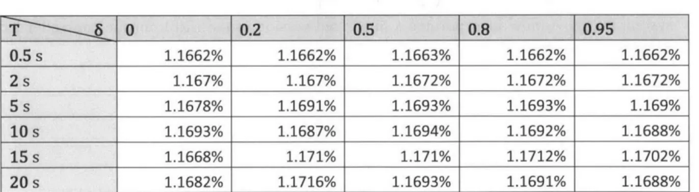
5.1 Sensitivity analysis of finite-horizon LQR parameters

The solution of the finite-horizon LQR problem depends on the solution horizon T and the control reset period TR, which is the amount of time that the current solution is actually being used by the controller before a new control reset. Of course TR T, and it is useful to define the overlap 6 ratio between the two periods:

TR

T

A number of simulations with the exact same wave elevation record (Hs = 6 m, Tm = 10.3 s)

have been performed at 10 m/s wind speed changing both the horizon T and the overlap, to see if there existed a strong trend indicating optimal solution parameters. Table 5.1 next

shows the results:

T

0

0.2

0.5

0.8

0.95

Table 5.1: Sensitivity of wave energy capture to horizon and overlap in a particular seastate at 10 m/s

It can be seen that yield stabilizes for horizons beyond 5-10 seconds. This is consistent with what is shown in other wave-energy extraction papers using dynamic programming [8], in which energy yield also stagnates for prediction horizons over a certain value. Overall it

seems most of the benefit of the unsteady LQR lies in being able to know the most immediate trend of the exciting force, and some additional benefit of it up to about one significant period Tm.

Overlap has also a marginal impact in energy yield, especially for shorter horizons where sensitivity to it is completely flat. It does however play a big role in computational demand. Choosing high overlap requires more frequent control resets and thus more computations.

Another factor to consider is the smoothness of the control input, with high overlap resulting in a smoother control input. Low overlap results in some degree of control chatter appearing, especially in the torque control (pitch control has far less marked jumps). Compared to the mean value these jumps are not so big and they can also be filtered, so they may not be very detrimental. Figure 5.1 shows the same fragment of simulation with different overlap values.

31 58 31 567 31 55 31 55 31 54 31 53 31 52 31 51 31 57 31 54 31 55 31.54 31 53 31 52 31 51 31 57 31 5 31 55 Z 31 54 31 53 31 52 31 51 22B 232 232 234 Is] 235 235 2411 242

Fig. 5.1: Sensitivity of torque input smoothness to overlap with T=10 s. Top graph 6=0.5, middle graph 6=0.9, bottom 6=0.99

It would appear then that choosing low overlaps provides the same energy yield with far less computational demand, which would be desirable as long as the control jumps can be smoothed out. Regarding horizon T, choosing a horizon length about the same duration than the mean wave period Tm seems to give good results as well. For the following sections, an overlap 8=0.5 (for faster computation time) and T = Tm will be used.

Generator Torque JL - --J - -- --- --- -- --

-5.2

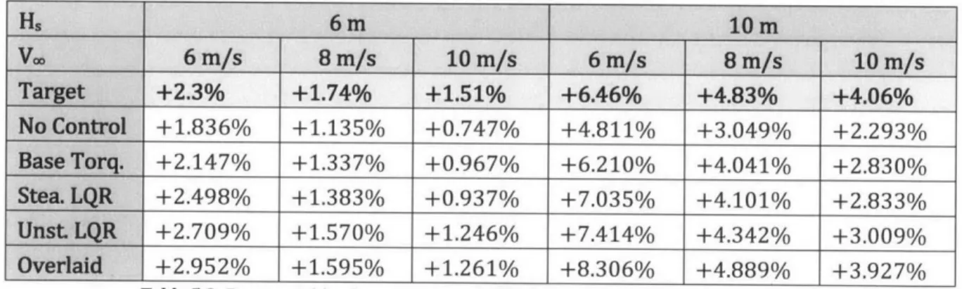
_{Results with different control options}

Table 5.2 offers a comparison of all the proposed control methods:

" _{No control: Keeps pitch at zero and torque at its constant mean value,}

TGen = TGen

Due to the movement of the platform, wave energy is captured even with constant control inputs.

* _{Base torque: Keeps pitch at zero and uses the quadratic control law for torque from} Section 4.3., following the specifications from the NREL documentation.

* _{Steady LQR: Variable pitch and torque, following the steady-state LQR formulation} from section 4.5.

* _{Unsteady LQR: Variable pitch and torque, following the finite-horizon LQR} formulation from Section 4.6.

* _{Overlaid control: Variable pitch decided by finite-horizon LQR and variable torque} that combines the baseline NREL torque controller with an additional variation decided by finite-horizon LQR, as described in section 4.7.

* _{Target: Values from Table 3.1, providing the upper bound for wave energy capture.}

Due to the stochastic nature of the problem, 10 simulations have been run for each case. The values from the table correspond to the mean of the ten simulations, but still some stochastic variation exists in the results.

Hs _{6 m 10 !i} VIM 6 m/s 8 m/s 10 m/s 6 m/s 8 m/s 10 m/s Target +2.3% +1.74% +1.51% +6.46% +4.83% +4.06% No Control +1.836% +1.135% +0.747% +4.811% +3.049% +2.293% Base Torq. +2.147% +1.337% +0.967% +6.210% +4.041% +2.830% Stea. LQR +2.498% +1.383% +0.937% +7.035% +4.101% +2.833%

Unst

Table 5.2: _{Energy yield enhancement result comparison for H, = 6 m and Hs = 10 m}

The overlaid control outperforms the other controllers in all cases, and even exceeds the target energy yield at lower wind speeds. Noteworthy is the fact that keeping constant pitch and torque already achieves significant energy capture, since surge oscillation alone can be expected to produce bigger energy yield due to the cubic equation for power.

The cubic law for power is well approximated by the second-order Taylor expansion as long as the deviations from the mean values are not too big, as shown by Figure 5.2. The fully nonlinear case has been computed by post-processing the results and extracting the real Cp values corresponding to the instantaneous tip-speed and pitch angle. Note that this is

referring to aerodynamic power and thus presents big power of the turbine is much more stable due to the rotor

Power over time

variations over time; the output inertia acting as a flywheel.

- _{second ord} cubic powe mean powe - - ----/ 240 245 250 255 260 Is] er power law r law r 265 270 275 280

Fig. 5.2: Comparison between the quadratic approximation of the aerodynamic power used for LQR and the post-processed equivalent power using the cubic law and real Cp values at wind speed 8 m/s.

Comparing the baseline torque controller inputs to the finite-horizon LQR inputs, they show very different behaviors. The finite-horizon LQR keeps very low torque variations compared to the NREL torque controller, but the pitch activity manages to extract more energy from the wind.

Generator Torque -~

~

_O

I0

0

Torque control activity in the finite-horizon LQR case could in theory be increased by reducing its cost in the R matrix, currently set to 0.1. However, matrix R is already very poorly conditioned and setting an even lower cost for the torque activity results in instability of the ODE system solution. Tuning of the cost matrices might be able to optimize energy capture further but it is not straightforward and this has not been attempted as part of the present work. A way around it is using the overlaid controller described in section 4.6, that combines both controllers. This results in torque activity that is basically similar to the baseline NREL torque controller with an added low amplitude variation set by LQR, while the pitch activity is kept similar to the unsteady LQR case.

The main mechanism seems to be the ability

[I 0,5 0.49 0.48 0. 47 0.46 0.45 0.44 410

to explain the differences in performance between the controllers to keep a higher Cp coefficient, as shown in Figure 5.4.

Cp coefficient over time

415

[s]

420 425 430

Fig 5.4: Power Coefficient comparison with Hs = 6 m

Surge velocity variation is almost the same in both cases, so the different Cp is the only parameter making a difference in energy yield. No controller is able to actually keep optimal tip-speed ratio since the rotational speed variations are not big enough to keep up with the changes in apparent wind speed due to surge. This implies that the finite-horizon LQR is setting the pitch angle to minimize drop in Cp when tip-speed ratio is away from optimal. When tip speed is near optimal, the Cp surface is flat and small changes in pitch do not affect

power capture.

Baseline NREL torque control Finite-horizon LQR

Overlaid control