Adaptive protocols for the quantum depolarizing channel

Adaptive Protocols for

the Quantum Depolarizing Channel

by

Alan W. Leung

B.A., The University of Cambridge, 2002

M.A., The University of Cambridge, 2006

Submitted to the Department of Mathematics

in partial fulfillment of the requirements for the degree of

Doctor of Philosophy

at the

MASSACHUSETTS INSTITUTE OF TECHNOLOGY

June 2007

@

Alan W. Leung, MMVII. All rights reserved.

The author hereby grants to MIT permission to reproduce and to

distribute publicly paper and electronic copies of this thesis document

in whole or in part in any medium known or hereafter created.

Author

....

A

uthor...

...

Department of Mathematics

May 1, 2007

Certified by... ... ...-...

...

...

...

Peter W. Shor

Morss Professor of Applied Mathematics

,

Thesii Supervisor

Accepted by ...

Alar Toomre

Chairman, Applied Mathejmatics C9mmittee

Accepted by ...

MASSAHUSETS I•tif

"

Pavel I. Etingof

Chairman, Department Committee on Graduate Students

pf$GfwfS

MASSACHUSETTS INSTIM.E OF TECHNOLOGY

JUN 0 8 2007

LIBRARIES

_{_ I__~ I} I

Adaptive Protocols for the Quantum Depolarizing Channel

by

Alan W. Leung

Submitted to the Department of Mathematics on May 1, 2007, in partial fulfillment of the

requirements for the degree of Doctor of Philosophy

Abstract

In the first part, we present a family of entanglement purification protocols that gen-eralize four previous methods, namely the recurrence method, the modified recurrence method, and the two methods proposed by Maneva-Smolin and Leung-Shor. We will show that this family of protocols have improved yields over a wide range of initial fidelities F, and hence imply new lower bounds on the quantum capacity assisted by two-way classical communication of the quantum depolarizing channel. In particu-lar, we show that the yields of these protocols are higher than the yield of universal hashing for F less than 0.99999 and as F goes to 1.

In the second part, we define, for any quantum discrete memoryless channel, quantum entanglement capacity with classical feedback, a quantity that lies between two other well-studied quantities. These two quantities - namely the quantum capacity assisted by two-way classical communication and the quantum capacity with classical feedback

- are widely conjectured to be different. We then present adaptive protocols for this newly-defined quantity on the quantum depolarizing channel. These protocols in turn imply new lower bounds on the quantum capacity with classical feedback.

Thesis Supervisor: Peter W. Shor

Acknowledgments

I am deeply indebted to my thesis advisor Peter Shor, without whom this thesis would not have been possible. I would like to thank him for being my advisor, his teaching, ingenious insights, meetings and discussions. All these are privileges I am very grateful for.

I would like to thank Prof. Seth Lloyd and Prof. Daniel J. Kleitman for serving on the thesis committee.

Over the years, many faculties contributed to my research, education and general well-being in the department, and I want to thank these professors. Among them are Prof. Rogers for working on 18.022 and RSI programs, Prof. Pak for passing my qualifying exam and research advising, Prof. Freedman for working on 18.03 and Prof. Hesselholt for working on 18.022. They are excellent researchers and also extraordinary folks to be acquainted with.

I would like to thank Joanne, Stevie and Debbie from the undergraduate math office for their helpfulness and friendliness. Thanks also go to Linda and Michelle from the graduate student office for their reminders and assistance in various administrative tasks.

I am grateful that during the past 5 years, I get to know many other talented graduate students and fabulous friends. Especially, Fu Liu, Thomas Lam, Huadong Pang and Joungkeun Lim. I thank them for encouragements and the joys and tears that we shared.

I would like to thank my parents and my sister Cary. Their undivided and un-conditional supports have made the overseas study in the UK and the pursuit of an

advanced degree in the US possible.

Finally, I want to dedicate the thesis to Vivian whose love has become my most important discovery, and the mystery and depth of which are oo."

Contents

1 Preliminaries 13

1.1 Introduction ... . .... ... . . . 13

1.2 Elementary notions in quantum information theory . ... 15

1.2.1 Quantum states ... 15

1.2.2 Quantum gates ... ... 16

1.2.3 Quantum measurements ... 17

1.2.4 Quantum discrete memoryless channel (QDMC) and its various capacities ... 19

1.3 Previous works ... 22

1.3.1 Universal hashing ... . . ... .. 22

1.3.2 The recurrence method and the modified recurrence method . 23 1.3.3 The Maneva-Smolin method . ... 24

2 Adaptive entanglement purification protocols 25 2.1 The Leung-Shor method ... .. 26

2.1.1 New protocol with improved yield . ... 26

2.1.2 Closed-form expression ... 27

2.2 Adaptive Entanglement Purification Protocols (AEPP) ... . 31

2.2.1 Description of AEPP ... 31

2.2.2 Generalization of previous methods . ... 35

2.2.3 Optim ization ... 37

2.2.4 Higher yield than universal hashing . ... 37

2.4 Modified AEPP ... 2.4.1 New-AEPP(a,4) ... 2.4.2 New-AEPP(a,N=2n) _...

2.4.3 Yield of New-AEPP(a,N= 2n_{) on the Werner state .}

2.5 Discussion on 2-EPP . ...

3 Quantum entanglement capacity with classical feedback

3.1 A quantity that lies between QB and Q2

3.1.1 Definition of EB . ...

3.1.2 EsB < Q2 ... ... 3.1.3 Q B

<

EB .. .... .. .. .... .. ...

3.1.4 EB as quantum backward capacity with classical 3.2 Adaptive quantum error-correcting codes (AQECC) . . 3.2.1 Stabilizer formalism for QECC . . . .

3.2.2 EB protocols via AQECC . . . . 3.2.3 Cat code and modified Cat code . . . .

3.2.4 Shor code ... ...

3.2.5 Modified recurrence method . . . . 3.2.6 Leung-Shor method . . . ..

3.3 New lower bounds on QB . . . ..

3.4 Threshold of Cat code . . . . . . . . ..

3.5 Discussion on QB, EB and Q2 . . . . ... feedback . . . . . 57 57 58 61 61 61 62 62 63 66 71 74 75 76 77 78 ' " ' " '

List of Figures

1-1 Single-qubit and two-qubit quantum gates. . ... 17

1-2 BXOR operation. ... . ... ... ... 18

1-3 The recurrence method. ... 23

1-4 The Maneva-Smolin method when m = 4. . ... 24

2-1 The Leung-Shor method. The yield of this protocol is shown in figure 2-2. . . . .... 26

2-2 The dotted line is the yield for modified recurrence method [7]; the dash line is for the Maneva-Smolin method [34]. The yield of our new method is represented by the solid line, and there is an improvement over the previous methods when the initial fidelity is between 7.5 and 8.45. ... . ... .. 29

2-3 AEPP(a,2) . ... . ... 32

2-4 AEPP(a,4) and AEPP(a,8). ...

..

33

2-5 AEPP(p,N=2) ... ... 35

2-6 Comparison of AEPP and previous methods: The lightly colored line is the yield of the four methods discussed in sec.2.2.1; the solid line represents the yields of AEPP(a,N = 2') where n = 2, 3, 4, 5, 6; the dashed line represents the optimized AEPP(a,4), which is denoted by AEPP*(a,4) (see section 2.2.3 for details). . ... . 36

2-7 The Maneva-Smolin method[34]... .. 37

2-8 The Leung-Shor method: section 2.1.1 and [32]. . ... 37

2-10 New-AEPP(a, N=2"). Alice and Bob replace measurements along Z-axis by universal hashing wherever the entropy of the qubit pair is less

than 1. ... ... .. 45

2-11 Yield of New-AEPP(a, N=2") on the Werner state PF for n = 2, 3, 4, 5, 6. 55 3-1 An EB protocols for channel Af(See the text for details). . ... 60 3-2 Encoding half of the EPR pair I(+) with a QECC . ... 65 3-3 4-bit Cat code in the language of entanglement purification protocols.

Note that in our protocols if Bob's measurement results do not agree with Alice's, then not all qubits will be sent through .p. Alice's mea-surement results are assumed to be all '+1' so Alice need not send Bob any classical information even though Bob 'compares' his results against Alice's. See the text for details. . ... 69 3-4 Lower bounds on EB(8p) via n-bit Cat code and modified Cat code.

See the text for details. ... ... . 70

3-5 4-bit Cat code vs. 4-bit modified Cat code. . ... . 71

3-6 Lower bounds on EB(Sp) via 9-bit Shor code and 9-bit Cat code .... 73 3-7 Lower bounds on EB ($) via the modified recurrence method. .... 74

3-8 Lower bounds on EB(8p) via the Leung-Shor method... . 75

3-9 Lower bounds on EB(p). . ... . 76 3-10 Lower bounds on QB(S) .)... . .. ... 77 3-11 Threshold fidelity F = 3

List of Tables

1.1 Outputs of the BXOR operations for Bell states 'source' (the top row) and 'target' (the leftmost column) inputs. . ... 18 2.1 The quantum states that lead to identical results for Alice and Bob.

Chapter 1

Preliminaries

1.1

Introduction

Quantum information theory studies the information processing power one can achieve by harnessing quantum mechanical principles[8, 35, 38]. Many important results such as quantum teleportation, superdense coding, factoring and search algorithms make use of quantum entanglements as fundamental resources[3, 11, 22, 41]. There is no complete theory to categorize and quantify the amount of entanglements in

N spin-! particles in general. Among the prominent measures are entanglement

cost, entanglement of formation, relative entropy of entanglement and distillable entanglement[14, 20, 21, 45].

In studying the entanglement-assisted capacities of a quantum discrete memoryless channel (QDMC) and the trade-offs between resources in attaining them, quantum entanglement is expressed in terms of an ebit - a pair of maximally entangled spin-1 particles -_{shared by the sender Alice and receiver Bob[9, 10, 18, 23, 40]. For example,}

00o: I4D)

=

(ITT) + 1Wl))

01 :

+

=

(ITI) + I+T))

10:

=

L(ITT)- j1j))

11: IT-) -- •([)- 11M}) (1.1)

are the so-called Bell basis and each of these states is considered equivalent to an ebit. However, these maximally-entangled pure states are only special cases of a general two-particle mixed state. In fact, any pure states, entangled or not, become mixed states once they are exposed to noise. Therefore, it is important to study procedures by which the sender and receiver can extract pure-state entanglement out of some shared mixed entangled states. These procedures are called entanglement purification protocols (EPP).

EPP are divided into 1-EPP and 2-EPP according to whether the sender and receiver are allowed to communicate uni- or bi-directionally. The scenario in which we study EPP is described as follows:

At the beginning of these entanglement purification protocols, Alice and Bob share a large number of the generalized Werner states[47]

1-F

PF = F '+) (+lI +

1

3 (

|-) (D-I + II+) (T+I +

IT-)

(T-I),

(1.2)

say p~O, and they are allowed to communicate classically, apply unitary transforma-tions and perform projective measurements. We place no restriction on the size of their ancilla systems so that we lose no generality in restricting their local operations to unitaries and projective measurements. In the end, the quantum states T shared by Alice and Bob are to be a close approximation of the maximally entangled states

(I'+)

((D+ l)®M, or more precisely we require the fidelity between T and (jV+) (D+|)®M

There are two main reasons why this is considered a general scenario. The first reason is, by a preprocessing operation known as "twirl", any two-particle mixed state can be converted to a classical mixture of the four Bell basis states, and this alone is sufficient as an input state to all the protocols discussed in this thesis[7]. However, it is more convenient to equalize three of the four Bell states and prepare the input as the Werner state PF, even though the equalization only adds unnecessary entropy to the mixture.

The second reason is the equivalence between an entanglement purification pro-tocol on the Werner state PF and a propro-tocol to faithfully transmit quantum states through the (4F-1)-depolarizing channel established in [7]. A p-depolarizing channel is a simple qubit channel such that a qubit passes through the channel undisturbed with probability p and outputs as a completely random qubit with probability 1 - p.

Specifically, the yield of a 1-EPP on the Werner state PF is equal to the unassisted quantum capacity of a (4F-1) depolarizing channel (Q); and the yield of a 2-EPP on the Werner state pr is equal to the quantum capacity assisted by two-way classical communication of a (4F-1) -depolarizing channel (Q2).

1.2

Elementary notions in quantum information

theory

In this section, we review some elementary notions in quantum information theory. Not only do they provide background materials, but also introduce notations to facil-itate discussion in this thesis. Most of these notations and discussions follow [30, 35].

1.2.1

Quantum states

As a postulate of quantum mechanics, one can associate any isolated physical system with a Hilbert space known as the state space of the system. The system is then completely characterized by a state vector. In quantum computation and quantum information theory, the conventional unit is a qubit - analogous to a classical bit in

classical information theory [16] - and its state is represented by a unit vector in a two-dimensional Hilbert space, -/2. Unlike its classical counterpart that has a state

of either 0 or 1, however, a qubit can be a linear combination of the basis states 10) and

I1).

For example, ao 10) + al I1) E H2 where ao and a, are complex numbers.

The basis states 10) and I1) are also known as the computational basis. In fact, we have already seen examples of a state vector in higher dimension. The state vector

I0

+ ) _{= -L(100) + Ill)), one of the four Bell states in (1.1), is in a four-dimensional}

Hilbert space, 'H4 - H2 0 7R2 and thus describes the state of two qubits.

The density operator language is very useful in describing quantum states that are not completely known[30]. For example, we use the notation

10)

(01 + 11) (11

to describe a qubit that has a probability 1 to be in the state 10) and a probability of 2 to be in the state 1). In general, if a quantum system has a probability of pi to be in the state 0i/) for i = 1, 2,..., n, then we say the system is an ensemble of pure states {pi, JVb)}Lj and is described by the density operator

n

P= AP Il i) (bil E B(7-ld) (1.3)

i=1

where

1j

) E

-d

and B(ld) is the bounded algebra on a d-dimensional Hilbert space. Mathematically, any operator p is the density operator associated to some ensemble {pi, I0i) } if and only if

1. p has trace equal to one; and 2. p is a positive operator.

1.2.2

Quantum gates

In this section, we introduce circuit notations for common quantum gates such as the single-qubit Pauli matrices and the two-qubit Controlled-NOT gate. We also illustrate the BXOR operation -bilateral application of Controlled-NOT on a bipartite quantum state -which will be used extensively. Note that all matrices in this section

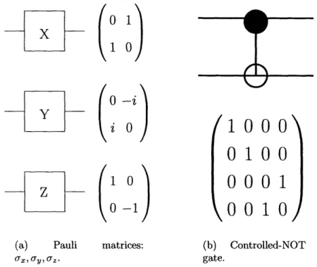
and throughout this thesis are expressed in the computational basis unless stated otherwise. In figure 1-1, we show examples of quantum gates that act on one or two qubits.

xt

(s

0 1

X0

(1

0

/

Y

z

(

(a) Pauli m (7, ay, a7 z -i 0 0 -1 latrices:

1000

0100

0001

0010

(b) gate. Controlled-NOT

Figure 1-1: Single-qubit and two-qubit quantum gates.

When we study entanglement purification of bipartite quantum states, we will often use the BXOR operation. Suppose two persons whom we call Alice and Bob share the two bipartite states 1(I+) and I4-), we say Alice and Bob apply BXOR on

14D+)

and j)-) and that I(+) is the 'source' and jI-) is the 'target' when the scenario in figure 1-2 occurs. In table 1.1, we list all possibilities of applying BXOR to the four Bell states in (1.1) as these will be useful in the discussion of entanglement purification protocols.

1.2.3

Quantum measurements

A projective measurement, a special case of what is known as POVW measurements,

Alice

source II+)

target

IJ<-)

Bob

Figure 1-2: BXOR operation.

input

K~)

jlJI+)

K)

I-)>

+ j+>) Ij->) I'+)

)

I-+>

) K-)

IT-)

I¢a-/

¢ > I¢

I+

ia-/

¢ / I¢ / I

-I'->) I -) I'

+

₎

I )- ID-) I -)

|K+)

141-)

(source) (target)

(source)

(target)

(source)

(target) (source) (target) Table 1.1: Outputs of the BXOR operations for

'target' (the leftmost column) inputs.

Bell states 'source' (the top row) and

would like to take a measurement. This Hermitian operator, also called an observable in this case, has a spectral decomposition,

M = E Pm,

m

where Pm is the projector onto the eigenspace of M with eigenvalue m. The different values of m are the possible measurement outcomes. If the quantum state is repre-sented by a state vector

[4),

then the probability of getting the measurement result

m is given by

prob(m) = (,0I Pm

[0)

-I'->

I|-)

Given that the measurement outcome is m, the quantum system immediately after the measurement is described by

Vprob(m)

For example, when the quantum state 10>+11> is measured by the observable uz = (+1) 10) (01 + (-1)

11)

(11, there is a probability 0.5 that the outcome is +1 and the quantum state is 10); and a probability 0.5 that the outcome is -1 and the quantum state is 11). When the observable is a. (or respectively az), we say we measure a quantum state along the x-axis (or respectively z-axis). In section 1.2.1, we learned that a mixed quantum state can be conveniently represented by a density operator

p. Then the probability of getting measurement result m is given by

prob(m) = tr(PtPmp)

and the quantum system immediately after the measurement is described by

P pP""

tr(Pt~Pmp)

1.2.4

Quantum discrete memoryless channel (QDMC)

and its various capacities

Discrete memoryless channel (DMC) can be described by a probability transition matrix and its capacity is uniquely defined[16, 38]. Quantum discrete memoryless channel (QDMC) can be described in many different ways and has various well-defined capacities depending on the availability of auxiliary resources such as classical communication or shared entanglements.

Mathematically, QDMC can be defined as a trace-preserving, completely positive linear map from the bounded algebra of an input Hilbert space to the bounded algebra of an output Hilbert space,

N: B(Nd,) - B(Na)2

and any such map

N

can be given an operator-sum representation [30, 35] which we state as follows,

N(p) = E EjpEý (1.4)

where {Ey} is a set of linear operators which map the input Hilbert space Nd, to the output Hilbert space 7_-t_d

2 and Ej EE = I. Hence if we represent a general input state as a density operator (c.f. equation (1.3)), the output state is

n

P=-Epii)(/iI P- = piEj p I'0i) (ViIE. (1.5)

i=1 i,j

The QDMC we study in this thesis is the quantum depolarizing channel. A p-depolarizing channel £p , : B(:(2) -- B(N 2) has the following set of linear operator

elements:

{Eo 3 p I, E = 4-x, E2 = • o• , E3 = =

Simple algebra shows that 3

(p) =Z E pE=p x p + (1 -p) x 7

j=0

i.e. with probability p the quantum state passes the channel unaffected and with probability 1 - p the quantum state is replaced by a completely random state 1.

the amount of information that can be transmitted asymptotically without error per channel use and that this value is unaffected by the use of classical feedback, for quantum discrete memoryless channels, the analogous statements are not true. Capacities are affected by side classical communication and shared entanglement[5, 9]; and QDMC can be used to transmit either classical or quantum information.

We can then define, for every quantum discrete memoryless channel, various ca-pacities: C, unassisted classical capacity; CB, classical capacity assisted by clas-sical feedback; C2, classical capacity assisted by independent classical information;

CE, entanglement-assisted classical capacity; Q, unassisted quantum capacity; QB,

quantum capacity assisted by classical feedback; Q2, quantum capacity assisted by independent classical information; and finally QE, entanglement-assisted quantum capacity. So far, some progress has been made to compute the capacities for spe-cific channels[6, 9, 27] and to study their relations[5]. However, search for a general formula only succeeded in a few cases[10, 17, 24, 37, 40], and progress in this direc-tion has been hindered by the additivity conjecture[39]. In particular, the following capacities (of the quantum depolarizing channel) will be studied in this thesis,

* C: the rate at which the sender can transmit classical information to the receiver asymptotically without error;

*

Q: the rate at which the sender can transmit quantum information to the receiver asymptotically without error;

* QB: the rate at which the sender can transmit quantum information to the

receiver asymptotically without error when a classical communication channel from Bob to Alice is available; and

* Q2: the rate at which the sender can transmit quantum information to the receiver asymptotically without error when a bidirectional classical communi-cation channel between Alice and Bob is available.

Whilst the first two capacities can easily be described mathematically, the last two capacities cannot because the protocols to achieve the capacities may be interactive,

i.e. Alice and Bob can communicate classically after each channel use. In this thesis, we will improve the lower bounds of the last two capacities for a p-depolarizing channel.

1.3

Previous works

In this section, we review the best known entanglement purification protocols, namely the universal hashing, the recurrence method and the Maneva-Smolin method. Uni-versal hashing is a 1-EPP and the last two methods are 2-EPP. As aforementioned, it is known that the yield of any 1-EPP on the Werner state PF is the same as the unassisted quantum capacity of a (4F1 -depolarizing channel (Q(&p)); and the yield of any 2-EPP on the Werner state pF is the same as the quantum capacity assisted by two-way classical communication of a (4F -depolarizing channel (Q2(Ep)).

1.3.1

Universal hashing

Universal hashing, introduced in [7], requires only one-way classical communication and hence is a 1-EPP. The hashing method works by having Alice and Bob each perform some local unitary operations on the corresponding members of the shared bipartite quantum states. They then locally measure some of the pairs to gain classical information about the identities of the the remaining unmeasured pairs. It was shown that each measurement can be made to reveal almost 1 bit of information about the unmeasured Bell states pairs. Since the information associated with a quantum state PF is given by its von Neumann entropy S(pF), we know from typical subspace argument that, with probability approaching 1 and by measuring NS(pF) pairs, Alice and Bob can figure out the identities of all pairs including the unmeasured ones. Once the identities of the Bell states are known, Alice and Bob can convert them into the standard states (D+ easily. Therefore this protocol distills a yield of (N -NS(pF))/N = 1 - S(pF).

1.3.2

The recurrence method and the modified recurrence

method

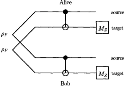
Alice PF PF source target soullrce target

Figure 1-3: The recurrence method.

The recurrence method[4, 7] is illustrated in figure 1-3. Alice and Bob put the quantum states pf g into groups of two and apply XOR operations to the correspond-ing members of the quantum states p 2_{, one as the source and one as the target.}

They then take projective measurements on the target states along the z-axis, and compare their measurement results with the side classical communication channel. If they get identical results, the source pair "passed"; otherwise the source pair "failed". Alice and Bob then collect all the "passed" pairs, and apply a unilateral 7r rotation

ax followed by a bilateral ir/2 rotation Bx1. This process is iterated until it becomes

more beneficial to pass on to the universal hashing. If we denote the quantum states by p = Poo •D+) (4+D +pol 'I+) (,+i+plo ID-) (I- J+pll |I-) (9-1, then this protocol has the following recurrence relation:

Po/ = (P20 + p20)/ppass; P1 (p021 - p21)/Ppss;

P1 0o = 2PoxP11/Ppass; P11 = 2pooPlo/Ppass; (1.6)

and

1

As mentioned in [7], the application of a oa and Bx rather than a twirl was proposed by C. Macchiavello. This is known as the modified recurrence method

Ppass - po + p P- + P + 2pooPio

+

2_{p01P11. (1.7)}

1.3.3

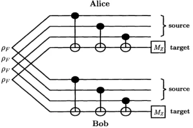
The Maneva-Smolin method

The Maneva-Smolin method[34] is illustrated in figure 1-4. Alice and Bob first choose a block size m and put the quantum states into groups of m. They then apply bipartite XOR gates between each of the first m - 1 pairs and the mth pairs. After that, they take measurements on these mth pairs along the z-axis, and compare their results with side classical communication channel. If they get identical results, they perform universal hashing on the corresponding m - 1 remaining pairs; if they get different results, they throw away all m pairs. The yield for this method is:

m-lI( - H(passed source states)

p••ss

-m m-1

where H(P) is the Shannon entropy of the probability distribution P.

Alice source SMz target P1 P11, Starget Bob

Chapter 2

Adaptive entanglement purification

protocols

In this chapter, we study 2-EPP, entanglement purification protocols when the two parties, Alice and Bob, are allowed to communicate classically. In section 2.1, we introduce a new 2-EPP [32]. We compute its yield for the Werner state PF and com-pare with the 2-EPP introduced in section 1.3. We also give a closed-form expression for general Bell-diagonal input states. In section 2.2, we present a family of 2-EPP that generalizes the previous methods in section 1.3 and the method in section 2.1. We show this family of protocols have improved yields over a wide range of initial fidelities F. In particular, the yield of this family of protocols on the Werner state PF is higher than that of universal hashing for F < 0.993 and as F -- oo. In section 2.3, we established the 'F - oc' part of the previous statement analytically. In section

2.4, we modify the family of protocols to achieve higher yields. Finally, we discuss the results of 2-EPP, some recent progresses[25, 46] and directions for further research.

Our protocols work for any Bell-diagonal states, and we adopt the 2-bit repre-sentation of the Bell states in (1.1). As a result, the Werner state pF is simply a probability distribution over the four Bell states, 00, 01, 10 and 11. Similarly, when Alice and Bob share N bipartite states that are Bell diagonal, a probability distrib-ution over a binary string of length 2N provides a complete description.

2.1

The Leung-Shor method

In section 2.1.1, we present a new entanglement purification protocol and compare its yield with the yields obtained by the recurrence method [7] and the Maneva-Smolin method [34]. In section 2.1.2, we give a closed-form expression for the yield of this new protocol.

2.1.1

New protocol with improved yield

Alice

It'

W W

Bob

Figure 2-1: The Leung-Shor 2-2.

method. The yield of this protocol is shown in figure

The new protocol is illustrated in figure 2-1. Alice and Bob share the quantum states pFN and put them into groups of four. They then apply the quantum circuit shown in figure 2-1 and take measurements on the third and fourth pairs along the x- and z-axis respectively. Using the side classical communication channel, they can compare their results with each other. If they get identical results on both measurements, they keep the first and second pairs and apply universal hashing[7]. If either of the two results disagrees, they throw away all four pairs.

The four pairs can be described by an 8-bit binary string, and since these are mixed states they are in fact probability distribution over all 256(= 28) possible 8-bit binary strings. The quantum circuit consists only of XOR gates and therefore maps the

'gook14 P, Am 14 P, I 1

P

,

8-bit binary strings, along with their underlying probability distribution, bijectively to themselves. Let us call these probability distributions P(ala2bib 2C1C2did2) and

P'(ala2blb2Cl C2dd 2).

The quantum measurements on the third and fourth pairs are simply checking the 5th bit (measurement on the third pair along x-axis) and the 8th bit (mea-surement on the fourth pair along z-axis), where a "0" means Alice and Bob get-ting identical results and a "1" means their getget-ting opposite results. For exam-ple, if the 8-bit binary string is "ala₂blb2clc2d1d2 = 00100111", which corresponds

to the quantum states D+(ID-T+T - , then Alice and Bob will get identical results on the third pair but opposite results on the fourth. The "pass" probability is

Ppass = Za,a2,bl,b2,c2,dlE{0,1} P'(a

l a

2bib20 c2d10) and the post-measurement

probabil-ity distribution is Q(ala2blb2) = -c 2,dlE{0,1} P'(ala2bib 2Oc2dO)/pa,,ss. The yield of

this method[34] is:

Ppass H(Q(aia2blb2)) (2.1)

where H(Q(ala2bib2)) is the Shannon entropy function. Figure 2-2 compares the yield

of our new method with the recurrence method and the Maneva-Smoline method.

2.1.2

Closed-form expression

The quantum circuit that Alice and Bob apply to the quantum states pf4 consists only of XOR gates and therefore maps the 8-bit binary strings bijectively to themselves. Let us call this bijection f:

f : {0,1}8 {0,1}8

(al, a2, b-, b2 7c1, c,2, d, d2) - (al

E

di, a2 G c2, bl E di, b2 G c2,

Table 2.1: The quantum states that lead to identical results for Alice and Bob.

G = (1 - F)/3; D+ = 00; x+ = 01; 1- = 10; - = 11.

P(ala2bib2clc2dld2) ala2blb2clc 2dld2 f(ala2bib2ClC2dld2) tr,d (f(ala2bib2Clc2dld2))

F4 00000000 00000000 0000 G4 01010101 00000100 0000 G4 10101010 00000010 0000 G4 11111111 00000110 0000 F2G2 00010001 00010000 0001 F2G2 01000100 00010100 0001 G4 10111011 00010010 0001 G4 11101110 00010110 0001 FzGz G4 F2G2 G4 FG3 FG3 FG3 FG 3 F2G2 F2G2 G4 G4 F2 G2 F2G2 G4 G4 00101000 01111101 10000010 11010111 00111001 01101100 10010011 11000110 00010100 01000001 10111110 11101011 00000101 01010000 10101111 11111010 00100000 00100100 00100010 00100110 00110000 00110100 00110010 00110110 01000100 01000000 01000110 01000010 01010100 01010000 01010110 01010010 0010 0010 0010 0010 0011 0011 0011 0011 0100 0100 0100 0100 0101 0101 0101 0101 F G2 00111100 01100100 0110 G4 01101001 01100000 0110 G4 10010110 01100110 0110 F2G2 11000011 01100010 0110 FG FG3 FG3 FG3 F2 G2 G4 F2G2 G4 F2 GC G4 G 4 F2G2 G 4 F2G2 G4 00101101 01111000 10000111 11010010 00100010 01110111 10001000 11011101 00110011 01100110 10011001 11001100 00001010 01011111 10100000 11110101 FGC FG3 FG3 FG3 FG3 FG 3 FG3 FG3 FG FG3 FG 3 FG3 FGW FG3 FG3 FG3 F 2G G4 G4 F2G2 01110100 01110000 01110110 01110010 00011011 01001110 10110001 11100100 00110110 01100011 10011100 11001001 00100111 01110010 10001101 11011000 00011110 01001011 10110100 11100001 00001111 01011010 10100101 11110000 0111 0111 0111 0111 10000010 10000110 10000000 10000100 10010010 10010110 10010000 10010100 10100010 10100110 10100000 10100100 10110010 10110110 10110000 10110100 11000110 11000010 11000100 11000000 11010110 11010010 11010100 11010000 11100110 11100010 11100100 11100000 11110110 11110010 11110100 11110000 28 1000 1000 1000 1000 1001 1001 1001 1001 1010 1010 1010 1010 1011 1011 1011 1011 1100 1100 1100 1100 1101 1101 1101 1101 1110 1110 1110 1110 1111 1111 1111 1111 --- --- ~---

---SRecurrence - - Maneva-Smolin - New method• 0.10 0.05 0.00 0.73 0.755 0.78 0.805 0.83 0.855

Initial Fidelity

Figure 2-2: The dotted line is the yield for modified recurrence method [7]; the dash line is for the Maneva-Smolin method [34]. The yield of our new method is represented by the solid line, and there is an improvement over the previous methods when the initial fidelity is between 7.5 and 8.45.

In table 2.1, we list the quantum states that lead to identical measurement results for both measurements and the associated probabilities in the ensemble pf4. From

that, we can write down expressions for Ppass and H(Q(ala₂bib2) in equation(2.1) as

follows: JI(Q(aia₂bib2)) = Ppass

--

(F

4

+ 3G

4

)

log

( F

4

+ 3G

4

_9(2F

2

_G

2

_{+ 2G}

4

_{) log}

₂ Ppass Ppass Ppass -6

(4FG

3 )o (4FG 3₎

Sppass

+ 2 _ppass F4 + 18F2_G2 + 24FG3 + 21G4

2F2G

+ 2G

4 Ppass (2.2) (2.3)

1--F

PF

= F

)

( + 3

+

+

however, our method works for any Bell-diagonal states

p = Poo Id+) ( + hI + Poel +) (b+c +e PlO I() ((i) + P1l 01 (T

-Equation (2.2) and (2.3) then become

H($QQlaj2bjb2a

(po

+-(Po

+

Pio

+

P¾11

(Poo

P io

+

P11

Ppass Ppass -6 x 4poOPolploPil )102 4poopolploP11 Ppass Ppass 2 1 + 2p2 2

2p

1 + 2p 2 -3 x 2p°0 2l 1O11 1092 log2Op11 Ppass Ppass

(2p

2o o 2p2 2p 2 oP + 2p 1 22 -3 x (2POp 2Pol10) log2 POPp 01)

Ppass Ppass

(2p

oP 1 + 2p 2o2 2 2 2 + 2p 1p 2

-3 x 0 110 log2 Pp11as 10

Ppass

Ppass

Ppass (P40 + Po P P + 41) + 6 x 4poopolploP1l + 3 x 2pIp i,jCe{O1}

2

i7j

With these equations, we can combine the recurrence method and our new method: we start with the recurrence method and pass on to our new method rather than universal hashing. Indeed, there are improvements, but they occur over segments of narrow regions and the improvements are insignificant. Therefore we believe these improvements have only to do with the number of recurrence steps performed before passing on to universal hashing, and we will spare the readers with the details.

2.2

Adaptive Entanglement Purification Protocols

(AEPP)

In this section, we will present a family of entanglement purification protocols that generalize four previous methods, namely the recurrence method, the modified recur-rence method, and the two methods proposed by Maneva-Smolin and Leung-Shor. We will show that this family of protocols have improved yields over a wide range of initial fidelities F, and hence imply new lower bounds on the quantum capacity assisted by two-way classical communication of the quantum depolarizing channel. In particular, the yields of these protocols are higher than the yield of universal hashing for F less than 0.993 and as F goes to 1.

The sender Alice and receiver Bob will often apply the BXOR operation on two of their N bipartite quantum states. These N states are mixtures of Bell diagonal states and can be represented by a probability distribution over a string of '0' and '1' of length 2N. Using the two classical bit notations, we write

BXOR(i,j) : {0, 1}2N -* {0, ₁}2N

(a , bi) - (ai D aj, bi)

(aj, bj) H (aj, bi G bj)

(ak, bk) _{(ak, bk) if k 4 i,j}

when Alice and Bob share apply BXOR to the ith pair as 'source' and the jth pair as 'target'.

2.2.1

Description of AEPP

1. AEPP(a,2): Alice and Bob put the bipartite quantum states pfN _{into groups of}

(al, bl, a2, b2) - (al E a2, bi, a2, bl D b2)

and take projective measurements on the second pair along the z-axis. Using two-way classical communication channel, they can compare their measurement results. If the measurement results agree(b1 D b2 = 0), then it is likely that there has been no

amplitude error and Alice and Bob will perform universal hashing on the first pair; if the results disagree(bi EDb2 = 1), they throw away the first pair because it is likely that

an amplitude error has occurred. We give a graphical representation of this protocol in figure 2-3. universal hashing tthrow away Figure 2-3: AEPP(a,2).

2. AEPP(a,4): Alice and Bob put the bipartite quantum states pON into groups of four, apply BXOR(1,4), BXOR(2,4), BXOR(3,4)

(al, bi, a2, b2, a3, b3, a4, b4)

(al E a₄, bl, a2 E a4, b2, a3 E a4, b3, a4, bl E b2 E b3 E b4)

and take projective measurements on the fourth pair along the z-axis. Using two-way classical communication channel, they can compare their measurement results. If the measurement results agree(b1 E b2 E b3 E b4 = 0), then it is likely that there has been

no amplitude error and Alice and Bob will perform universal hashing on the first three pairs together.

On the other hand, if the results disagree(b1 E b2 E b3 E b4 = 1), it is likely that

They do so by applying BXOR(2,1)

(al

E

a4, bl, a2

D

a4, b2, a3

@

a4, b3, a4, 1)

(al E a4, bl

D

b2, a

ED

a2, b2, a3 E a4, b3, a4, 1) (2.4)

and taking projective measurements on the first pair along the z-axis. Note that the second pair(al D a2, b2) and the third pair(a3 E a4, b3) are no longer entangled.

Alice and Bob then use classical communication channel to compare their results. If the results agree(b1 E b2 = 0), then the amplitude error detected by the first

measurements is more likely to be on either the third or the fourth pair than on the first two. Therefore Alice and Bob perform universal hashing on the second pair and throw away the third pair. If the results disagree(bl E b2 = 1), then the amplitude

error is more likely to be on the first two pairs. In this case, Alice and Bob perform universal hashing on the third pair and throw away the second pair.

Note that the amplitude error could have been on the fourth pair but this protocol works well even if that is the case; and also that with this procedure we always end up with one pair on which Alice and Bob can perform universal hashing when the first measurement results disagree. We represent this protocol graphically in figure

2-4(a). (hriaersaI iiniversal hashing 4 a• gniversal hashing 3a iversal shing tbrow hrow away away

(a) AEPP(a,4) (b) AEPP(a,8)

Figure 2-4: AEPP(a,4) and AEPP(a,8).

eight, apply BXOR(1,8), BXOR(2,8), BXOR(3,8), ... , BXOR(7,8)

(al, bl, a2, b2, * • , a7, b7, as, bs)

-(al E as, bl, a2 6 a8, b2, ... , a7 6 a8, b7, as, bl D ...

@

bs)

and take projective measurements on the eighth pair along the z-axis. Using classical communication channel, Alice and Bob compare their measurement results. If the

results agree(bl @... ED b8 = 0), then an amplitude error is not likely and they perform

universal hashing on the first seven pairs together.

On the other hand, if the measurement results disagree(b1 ED ... ED b8 = 1), then

Alice and Bob want to catch this amplitude error and they do that by applying BXOR(2,1), BXOR(3,1), BXOR(4,1)

(al E as, bi, a2 6 a8, b2, . . , a₇ 6) a₈, b₇, as, 1) I (al E as, bi E b₂ E b3 E b4, a1 E a2, b2, a1 D a3, b3,

al ED a4, b4, a5 ED a8, b5, a6 E as, b6, a7 D a8, b7, as, 1)

and taking projective measurements on the first pair along the z-axis. Note that the second, third and fourth pairs are not entangled with the fifth, sixth and seventh pairs. After Alice and Bob compare their results with classical communication channel and if the results disagree (bl ED b2 D b3s b4 = 1), they perform universal hashing on the

fifth, sixth and seventh pairs because bl ED b2 ED b3 b4 = 1 and bl ED ... ED b8 = 1

together imply b5 ED b6 ED b7 D b8 = 0. The first four pairs are now represented by

(al ED as, 1, al ED a2, b2, al ED a3, b3, al ED a4, b4), and it can be easily seen that we are in

the same situation as the left hand side of equation (2.4): Alice and Bob know that

bl ED b2 D b3 E b4 = 1 and the pair on which they measured to find out this information

has its phase error added to the other three pairs. Therefore Alice and Bob can apply the same procedure as equation (2.4) and end up with one pair that they will perform

universal hashing on. Now if the results actually agree (bl E b2 b3 3b4 = 0), the same

procedure still applies but we need to switch the roles played by the first four pairs and by the last four pair. We represent this protocol graphically in figure 2-4(b). 4. AEPP(a,N=2n_{) and AEPP(p,N=2n): Clearly, the above procedures}

general-ize to AEPP(a,N=2n_{) and can be proved inductively. The procedures}

-AEPP(a,N=2n)

- we discussed so far focus on amplitude error. If we instead try to detect phase er-ror by switching the source pairs and target pairs in all the BXOR operations and measuring along the x-axis rather than the z-axis, AEPP(p,N=2n) can be defined analogously. We represent the protocols AEPP(p,N=2") graphically in figure 2-5, and we present the yields of AEPP(a,N = 2n) for n = 2, 3, 4, 5, 6 in figure 2-6.

universal 27. hashing universal 2 1- 1 p hashing 2 - -universal 271-1 - 1 hashing universal hashing throw away Figure 2-5: AEPP(p,N=2n).

2.2.2

Generalization of previous methods

We show that, four previous protocols -the recurrence method, the modified recurrence method and the two methods proposed by Maneva-Smolin and Leung-Shor -all belong to the family AEPP(a/p,N = 2n).

1. The recurrence method: The recurrence method[7] is the repeat applications

of AEPP(a,2). When Alice and Bob have identical measurement results, rather than applying universal hashing right away, they repeatedly apply AEPP(a,2) until it is more beneficial to switch to hashing.

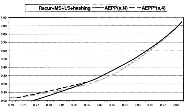
... Recur+MS+LS+hashing - AEPP(a,N) - - AEPP*(a,4) 1.00 0.90 0.80 0.70 0.60 .. 0.50 0.40 0.30 .. 0.20 0.10 0.00 0.73 0.75 0.77 0.79 0.81 0.83 0.85 0.87 0.89 0.91 0.93 0.95 0.97 0.99

Figure 2-6: Comparison of AEPP and previous methods: The lightly colored line is the yield of the four methods discussed in sec.2.2.1; the solid line represents the yields of AEPP(a,N = 2n) where n = 2, 3, 4, 5, 6; the dashed line represents the optimized AEPP(a,4), which is denoted by AEPP*(a,4) (see section 2.2.3 for details).

2. The modified recurrence method: The modified recurrence method[7] is

the repeat, alternate applications of AEPP(a,2) and AEPP(p,2). After Alice and Bob apply AEPP(a,2) and obtain identical measurement results, rather than apply-ing universal hashapply-ing right away, they repeatedly and alternately apply AEPP(p,2), AEPP(a,2) and so forth until it becomes more beneficial to switch to universal hash-ing.

3. The Maneva-Smolin method: The Maneva-Smolin method[34] is to apply the

first step of AEPP(a,N). Perform universal hashing on the N-i pairs if the measure-ment results agree but throw away all the N-1 pairs if they do not. This is illustrated in figure 2-7.

4. The Leung-Shor method: The Leung-Shor method(section 2.1.1 and [32]) is a

combination of the first step AEPP(a,4) and AEPP(p,4); however, this method fails to utilize all entanglements by throwing away the 3 pairs if the first measurement results disagree. This is illustrated in figure 2-8.

mrsal ng

throw

away

Figure 2-7: The Maneva-Smolin method[34].

universal hashing 3 4 a throw away throw away

Figure 2-8: The Leung-Shor method: section 2.1.1 and [32].

2.2.3

Optimization

After we apply AEPP(a,N=2'), we might end up with either 2n -1 pairs or n-1 groups

of pairs (2n - 1 - 1, 2n- _{2 - 1, ... 2}k _{- 1, ... 3 and 1) pairs depending on the results of the}

first measurements. It is possible to treat these n-1 groups differently because they are not entangled to each other. We can either perform universal hashing(as in the Maneva-Smolin method) or apply AEPP(p,2k - 1)(as in the Leung-Shor method). If we do apply AEPP(p,2k - 1), we will end up with two groups of quantum states of different sizes because we started with N = 2k - 1 rather than N = 2k. In figure 2-9,

we show two such possibilities as shown for N = 4 , and higher yields are achieved for F > 0.74 as shown in figure 2-6.

2.2.4

Higher yield than universal hashing

As we can see from figure 2-6, the yields of AEPP(a,N = 2n) exceed the yield of universal hashing for F < 0.993. In section 2.3, we prove the following theorem:

4z

/Figure 2-9: AEPP*(4,a). Figure 2-9: AEPP*(4,a).

Theorem 1. Let N = 2n _{where n is a positive integer.}

of AEPP(a,N) on the Werner state PF. Then

x(1

N/4 - 1 - x N

1

_{(1 + SNi_)}

-N SN-1 N- i SN -1₄ N/4 - 1 2- 1 N

Denote by YAEPP the yields

SN_

N/2-1

(1

Si 2-1 1

p(n+1+

Sl_ + S!Ny +-.. +.S3A+S1) N - 4

where p = prob(bl @b2 (a... .b = 0) and SK-1 = H(al aK, bl, a2 -aK, b2, -. , aK-1 (

Furthermore, let F = 2-1 and aK, bK-1|b, D ... ( bK = O) for K = 2, 4, 8,..., 2".

G = 1-F ₃ Then

lirn YAEPP >

n--o00 1 - H(F, G, G, G) +

> 1- H(F, G, G, G)

= Yield of universalhashing on PF

0

(Th N-i YAEPP = P XN N

H(p*) - p*

N K kL2 01 N/2 - 1 +(-p) x N121N x

-p* = lim p= n---oo

1

4

S(1 + e -).

2

2.3

Proof of theorem 1

Lemma 1. p* = lim prob(bx D b2 . n--oo 1

1

+ e3).

2

Proof. bi's are the amplitude error bits and, for any i, prob(bi = 1) = 2G = '

When we have N qubit pairs,

prob(no error) = prob(1 error) = 2 N

3N)

N(1

2)N1

3N

(2)

3N 2 N-1 2e2/3

3N

3

(2.5)

(2.6)

prob(2 errors) = N(N - 1) 2 ) N-1 (2 )2

3N

3N

N- (

prob(k errors) = 32 )-2 (2/3)2 N(N-1)... (N - k + 1) 2 )

3N

2

-k 3N

(2/3)

2

_-2/3

2!

(2/3)k

2

k!1

-kc! 3P -(2/3)k + O

(2.8)

N))

In equation (2.5), (2.6) and (2.7), we did not include the error term O ) because - (2/3) k 2 is negligible. In the following calculation, we will drop the error terms

for brevity.

where

(2.7)

e-2/3

lim l--+ oo p = prob(bl D b2 G ... bN = 0) (2/3)k -2/3 k! k is even 1 (2/3)k 2/3 (-2/3)k k=O e-2/3 (2/3)k (-2/3)k 2 k! + k! 1 k= 1 +- e4/3 p ) -2/3)

Lemma 2. For K = 2, 4, 8,..., 2", let

SK-1 = H(al a K, bl,a 2 ® aK, b2, . . ,aK-1 D aK, bK-1Ibl ... bK = 0) and

TK-1 = H(al

D

aK, bi, a2

(D

aK, b2,... , aK-1

D

aK, bK-1bl

b

...

D

bK = 1).

Then

N x H(F, G, G, G) > H(p, 1 - p) + pSN-1 + (1 - p)TN_1 and TK-1 > SK/2-1 + TK- + 1₂

(2.9)

(2.10)

Proof. To prove (2.9), note that N x H(F, G, G, G) = S(p~N). Let p = prob(b 1b 2 6

. . bN = 0). Then we can write pF = p x Po + (1 - p) x pl, where po is the state whose

support lies on Bell states that are characterized by bl

a

b2 e ... . b= 0 and p, is the

state whose support lies on Bell states that are characterized by bl D b2 G ... bN = 1.

It is clear then Po and p, have orthogonal supports as any two distinct Bell states

are. Then we have

N x H(F, G, G, G) = S(pfN)

= S(p x po + (1 -p) x p1)

= pS(po) + (1 - p)S(pi) + H(p)

= pH(al, bi, a2,..., bN-, aN, bbl ... E b = 0) +

(1 - p)H(al, bl, a2,..., bN_1, aN, bNIbl (... b = 1) + H(p)

= pH(al E aN, bl,..., aN-1 (D aN, bN-1, aN, bl E ... E bNIbl E ... E bN = 0) +

(1 - p)H(al E aN, bl,..., aN-1 D aN, bN-l, aN, bl E ... E bNI

b, ED... E bN = 1) + H(p) (2.11)

where the last equality holds because the operations BXOR(1, N), BXOR(2, N) ... BXOR(N - 1, N) are all unitary and hence preserve entropy. Since the function -p log2 p is subadditive for p < 1, we have

SN-1 - H(al E aN, bl,...,aN-1 E aN, bN-11Ibl ... E bN = 0)

< H(al D aN, bl, ... , aN-1 E aN, bN-l, aN, bl ED ... bNbl ED ...

e

bN = 0) and TN-1 -- H(al E aN,bl,..., aN-1 aN, bN-11b• E... E bN = 1)

< H(ai @ aN, bl,..., aN-1 E aN, bN-1, aN, bl E ... E bNIbl E... DbN = 1).

Substituting these into equation (2.11) yields N x H(F, G, G, G) > H(p) + pSN-1 +

(1 - p)TN-1.

To prove (2.10), note that for K qubit pairs shared between Alice and Bob

where K = _{2,4,8,..., N, when they apply the unitary operations BXOR(1, K),}

BXOR(2, K) ... BXOR(K - 1, K) and get different results for measuring the Kth

described by S(F) = H(al D aK, bl,..., aK-1 D aK, bK-lbl D... bK = 1)). symmetry, prob (b,

a...

. bK/2 = 1) = prob (bK/2+1 E ...

D

bK = 1) = 1. Therefore,

F (b...bK/2=1) + (bK/ 2+1j...ebK=1) where F(ble... bK/2=l) and F(bK/2+1e.ebK=1) have orthogonal supports:

TK-1 H(al

H (

aK, bl,...., aK-1 aK, bK-lIbl

E...

bK = 1)

= S(r)

SS( (b,,...(bK/2=1)

2

+

2v/Zl··mK-r

(bK/2+1(...EbK=l)

=- S F(bl ..-. bK/2= 1)) + IS F(bK/2+1l...®bK=l))

(2.12)

Note that

S(F(b~e...EbK/2=1))

= H(a1 E aK, bl,..., aK-1 aK, bK-1 (b1 ...

= H(al E aK, bl E... E bK/2, a2 al, b2, ... aK/: bK/2+1,... aK-1 0D aK, bK-l (b,

E

... E bK/2 = bK/2 = 1) A (bK/2+1 e .. 2

D

a1, bK/2, aK/2+1 D aK, 1) A (bK/2+1 E ... E bK =

.

EbK

=

0))

o))

= H(alOaK, bl ... bK/2, a2 1,b2,... , aK/2a1, bK/2(b ₁ E...bK/2

H

(aK/ 2+l

D

aK, bK/2+1, .... aK-1 aK, bK-1 (bK/2+1

ED

...

E

bK = 0))

= H(al aK, bl E ... bK/2, a2 E al, b2,..., aK/E al, bK/2 2 (bl

+SK/2-1

E

... (E bK/2 =

(2.13)

1)) (2.13)

where the second equality was obtained by applying the operations BXOR(2, 1), BXOR(3, 1),..., BXOR(K/2 - 1, 1), BXOR(K/2, 1). And since -p log2 p is

subad-ditive for p < 1, the first term in (2.13)

H(at ~ aK, bl ... bK/

2

,a2

b2,

l,

...

aK/2 al,

bK/

2

(b

...

bK/

2

1))

Ž H(a2a 1, b2, *aK/2 al, bK/₂ (b _{... ED bK/2=1))}

=

TK/2-1. (2.14)

Therefore, S(F(bl®...EbK/2=1)) TK/2+1 + SK/2-1. Using similar argumnts, one can show S ((bK/ ₂+±e ... bK•l ) > SK/2-1 +TK/2+1. Putting these back to equation (2.12),

TK-1

- _{S IF(bl ... EbK/2=1)}

>

-

(TK/2+1 + SK/2-1)

-2

= SK/2-1 + TK/2-1+ 1.

We are now ready to prove theorem 1. We first apply the above lemmas:

Nx H(F, G, G, G) > H(p) + pSN-1 + (1 - p)TN-1 > H(p) + pSN1 + (1 -> H(p) +pSN-1 + (1 -> H(p) + pSN1 + (1 -p) (1 + SN/2-1 + TN/2-1) p) (1 + SN/2-1 _{+ TN/4-1)} p) ((n- 1) + SN/2-1 + SN/4-1 + ... + S3 + S1

+ S

(F(bK/2+1e ...EbK=l)

+

_H()

1 +

2

(SK/2-1 +TK/2+I) 1

+

1 + SN/4-1

+T

₎

ipSN-1+(1-p)(SN/2-1+. .- .+Si+S _{NxH(F, G, G, G)-H(p)-(1-p) (n-+T)}

Simple calculation shows T, = 2. Therefore,

YAEPP = -(1 + SN-1) - N (n + 1 + SN/2-1 + SN/4- 1+ .+ S3 + Sl) N N p 1-p p 1-p = 1 - (n + 1) SN-1 (SN/2-1 + .+ S3 + S) N N N N 1p 1-p ) 1 I- 1 g (n+ 1) - N x H(F, G, G, G) - H(p) - (1 - p)(n - 1 + Tj) N N N H(p) - p > 1 -H(F, G, G, G) + N N

> 1 - H(F, G,

G,

G).

This completes the proof of theorem 1.

2.4

Modified AEPP

In this section, we modify AEPP from the previous section to achieve higher yields. Recall that, as the first steps of AEPP(a,N=2n), Alice and Bob apply BXOR(1, N),

BXOR(2, N), ... , BXOR(N - 1, N) to obtain the quantum state (al @ aN, bi, a2 &

aN, b2, ... , aN-1 ( aN, bN-1, aN, bl D b2 (D ... bN-1 @ bN) and take measurements on

the Nth qubit pair, (aN, bl @ b2 E ... E bN-1 D bN). However, if the entropy of the

Nth qubit pair is small, or more precisely if S(aN, bl @ b2 E ... D bN-1 D bN) < 1,

they can perform universal hashing instead of taking measurements along the z-axis. Specifically, Alice and Bob can apply AEPP(a,N=2") to M blocks of N qubit pairs and apply universal hashing to the M Nth qubit pairs as shown in figure 2-10. This modification has two immediate advantages:

-S(aN, b b

2

e

...

e

bNl

E

bN))/N.

2. Taking measurements in the original AEPP protocols destroys the information

in aN. However, universal hashing not only reveals the identity of bl E b2 ... @

bN-1EGbN but the value of aN as well. As a result, if aN = 0 and bl ... DbN = 0, the N-1 remaining qubit pairs are represented by (al, bl, a2, b2,... , aN-1, bN-1);

and if alv = 1 and bl E.. .Eb = 0, the qubits are represented by (al, 1, bl, a2ED

1, b2,... , aN-1 ( 1, bN-1). Alice and Bob can collect a large number of these

two distinct groups and apply universal hashing separately. By the concavity of entropy function, S(plp1 + P2P2) plS(pl) + p1 2S(p2), the entropy is smaller

and hence a higher yield will be obtained by hashing.

M blocks of N qubit pairs

N qubit pairs a, (D aN bl a2 ® aN b2 aN.-1 D aN bN-1 aNr bl ( ... e bN N qubit pairs ai D aN a2

e

aN b2 aNl-1 E aN bN-1 aN bl D ... G bN 1111111 I I 31111111I I N qubit pairs a (9 aN b, a2 G aN b2 aN-1 E aN bN-1 aN bl ( ... G bN

Figure 2-10: New-AEPP(a, N=2n). Alice and Bob replace measurements along Z-axis by universal hashing wherever the entropy of the qubit pair is less than 1.

In AEPP(a, N=2n), there are n - 2 more measurements if the first measurement

reveals bl ... E bN = 1. Obviously we should also replace these measurements by

hashing whenever possible, and take measurements only if the entropy of the qubit universal hashing