An Adaptive Partitioning Scheme for Ad-hoc and
Time-varying Database Analytics
by
Anil Shanbhag
B.Tech. in Computer Science
Indian Institute of Technology Bombay, 2014
Submitted to the Department of Electrical Engineering and Computer
Science
in partial fulfillment of the requirements for the degree of
Master of Science in Electrical Engineering and Computer Science
at the
MASSACHUSETTS INSTITUTE OF TECHNOLOGY
June 2016
c
Massachusetts Institute of Technology 2016. All rights reserved.
Author . . . .
Department of Electrical Engineering and Computer Science
May 19, 2016
Certified by . . . .
Samuel Madden
Professor of Electrical Engineering and Computer Science
Thesis Supervisor
Accepted by . . . .
Leslie A. Kolodziejski
Chairman, Department Committee on Graduate Students
An Adaptive Partitioning Scheme for Ad-hoc and
Time-varying Database Analytics
by
Anil Shanbhag
Submitted to the Department of Electrical Engineering and Computer Science on May 19, 2016, in partial fulfillment of the
requirements for the degree of
Master of Science in Electrical Engineering and Computer Science
Abstract
Data partitioning significantly improves query performance in distributed database systems. A large number of techniques have been proposed to efficiently partition a dataset, often focusing on finding the best partitioning for a particular query work-load. However, many modern analytic applications involve ad-hoc or exploratory analysis where users do not have a representative query workload. Furthermore, work-loads change over time as businesses evolve or as analysts gain better understanding of their data. Static workload-based data partitioning techniques are therefore not suitable for such settings. In this thesis, we present Amoeba, an adaptive distributed storage system for data skipping. It does not require an upfront query workload and adapts the data partitioning according to the queries posed by users over time. We present the data structures, partitioning algorithms, and an efficient implementation on top of Apache Spark and HDFS. Our experimental results show that the Amoeba storage system provides improved query performance for ad-hoc workloads, adapts to changes in the query workloads, and converges to a steady state in case of recurring workloads. On a real world workload, Amoeba reduces the total workload runtime by 1.8x compared to Spark with data partitioned and 3.4x compared to unmodified Spark.
Thesis Supervisor: Samuel Madden
Acknowledgments
I would like to thank Alekh Jindal, Qui Nguyen, Aaron Elmore, Jorge Quiane and Divyakanth Agarwal who have contributed many ideas to this work and helped build the system.
I would also like to thank Prof. Samuel Madden, my thesis supervisor, for being a constant source of guidance and feedback in this project and outside.
Finally, I am always grateful to my family and friends, who encouraged me and supported me along the way.
Contents
1 Introduction 13
2 Related Work 17
3 System Overview 21
4 Upfront Data Partitioning 23
4.1 Key Ideas . . . 24
4.2 Upfront Partitioning Algorithm . . . 27
5 Adaptive Repartitioning 31 5.1 Workload Monitor and Cost Model . . . 32
5.2 Partitioning Tree Transformations . . . 33
5.3 Divide-And-Conquer Repartitioning . . . 36
5.4 Handling Multiple Predicates . . . 39
6 Implementation 41 6.1 Initial Robust Partitioning . . . 41
6.2 Query Execution . . . 43
7 Discussion 45 7.1 Leveraging Replication . . . 45
7.2 Handling Joins . . . 46
8 Evaluation 47 8.1 Upfront Partitioning Performance . . . 47
8.3 Amoeba on Real Workload . . . . 53
9 Conclusion 55
Appendices 60
List of Figures
1-1 Example partitioning tree with 8 blocks . . . 14
3-1 Amoeba Architecture . . . 21
4-1 Partitioning Techniques. . . 25
4-2 Upfront Partitioning Algorithm Example. . . 26
5-1 Node swap in the partitioning tree. . . 34
5-2 Illustrating adaptive partitioning when predicate A2 appears repeatedly. 35 5-3 Node pushdown in partitioning tree. . . 35
5-4 Node rotation in partitioning tree. . . 35
7-1 Heterogenous Replication. . . 45
8-1 Ad-hoc query runtimes for different attributes of TPC-H lineitem. . . 48
8-2 Comparing the upload time in Amoeba with HDFS . . . . 49
8-3 Comparing performance of upfront partition tree vs kd-tree . . . 49
8-4 Query runtimes for changing query attributes on TPC-H lineitem. . . 51
8-5 Query runtimes for changing predicates on the same attribute of TPC-H lineitem. . . 52
8-6 Cumulative Optimizer Runtime Across 100 queries . . . 52
8-7 Cumulative Repartitioning Cost . . . 52
8-8 Total runtimes of the different approaches . . . 53
List of Tables
5.1 The cost and benefit estimates for different partitioning tree
Chapter 1
Introduction
Collecting data is increasingly becoming easier and cheaper, leading to ever-larger datasets. This big data, ranging from sources such as sensors to server logs has the potential to uncover business insights and help businesses make informed decisions, but only if they can analyze it effectively. For this reason, companies have adopted distributed database systems as the go-to solution for storing and analyzing their data.
Data partitioning is a well-known technique for improving the performance of distributed database applications. For instance, when selecting subsets of the data, having the data pre-partitioned on the selection attribute allows skipping irrelevant pieces of the data, i.e., without scanning the entire dataset. Joins and aggregations also benefit from data partitioning. Because of these performance gains, the database research community has proposed many techniques to find good data partitioning for a query workload. Such workload-based data partitioning techniques assume that the query workload is provided upfront or collected over time [1, 2, 3, 4, 5, 6, 7]. Unfortunately, in many cases a static query workload may not be known a priori.
One reason for this is that modern data analytics is data-centric and tends to in-volve ad-hoc and exploratory analysis. For example, an analyst may look for anoma-lies and trends in a user activity log, such as from web servers, network systems, transportation services, or any other sensors. Such analyses are ad-hoc and a repre-sentative set of queries is not available upfront. To illustrate, production workload traces from a Boston-based analytics startup reveal that even after seeing 80% of the
A4 B5 D4 1 2 D5 3 4 C6 B3 5 6 D4 7 8
Figure 1-1: Example partitioning tree with 8 blocks
workload, the remaining 20% of the workload still contains 57% new queries. These workload patterns are hard to collect in advance. Furthermore, collecting the query workload is tedious as analysts would typically like to start using data as soon as possible, rather than having to provide a workload before obtaining acceptable per-formance. Providing a workload upfront has the further complexity that it can overfit the database to that workload, requiring all other queries to scan unnecessary data partitions to compute answers.
Distributed storage systems like HDFS [8] store large files as a collection of blocks of fixed size (for HDFS the blocks size is usually 64/128MB). A block acts as the smallest unit of storage and gets replicated across multiple machines. The key idea is to exploit this block structure to build and maintain a partitioning tree on top of the table. A partitioning tree is a binary tree which partitions the data into a number of small partitions of roughly the size of a block. Each such partition contain a hypercube of the data. Figure 1-1 shows an example partitioning tree for a 1GB dataset over 4 attributes with block size 128MB. The data is split into 8 blocks, the same as what would be created by a block-based system, however each block now has additional metadata. For example, block 1’s tuple satisfy A ≤ 4 & B ≤ 5 & D ≤ 4. This results in it being possible to answer any query by reading a subset of partitions. The partitioning tree is improved over time based on queries submitted by the user. We implemented this idea in Amoeba. Amoeba is designed with three key properties in mind: (1) it requires no upfront query workload, while still providing good performance for a wide range of ad-hoc queries; (2) as users pose more queries over certain attributes, it adaptively repartitions the data, to gradually perform better on queries over frequent attributes and attribute ranges; and (3) it provides robust performance that avoids over-fitting to any particular workload.
The system exposes a relational storage manager, consisting of a collection of tables, with support for predicate-based data access i.e. scan a table with a set
of predicates to filter over. For example, executing scan over table employee with predicate age ≥ 30 and 1000 ≤ salary ≤ 2000. The data stored is partitioned and as a result we end up accessing a subset of the data. The system is self-tuning and as users start submitting queries to the system, it specializes the partitioning to the observed patterns over time.
Query optimizers tend to push predicates down to scan operator and big data systems like Spark SQL [9] allow custom predicate-based scan operators. Amoeba integrates as a predicate-based scan operator and the re-partitionings’ happening to change data layout are invisible to the user.
Adaptive partitioning/indexing is extensively used in modern single node in-memory column stores for achieving good performance. These techniques, called Cracking [10] have been used to generate adaptive index on a column based on in-coming queries. Partial sideways cracking [11] extends it to generate adaptive index on multiple columns. Cracking happens on each query and maintains additional
structures to create the index. The reason cracking cannot be applied to a
dis-tributed setting is because the cost of re-partitioning is very high. Each round of re-partitioning needs to be carefully planned to amortize the cost associated with it. Our approach is complementary to many other physical storage optimizations. For example, decomposed storage layouts (i.e., column-stores) are designed to avoid reading columns that aren’t accessed by a query. In contrast, partitioning schemes, including ours, aim to avoid reading entire partitions of the dataset. Although our prototype does not use a decomposed storage model, there is nothing about our approach that cannot work in such a setting: individual columns or column groups could easily be separately partitioned and accessed in our approach.
In summary, we make the following major contributions:
• We describe a set of techniques to aggressively partition a dataset over several attributes and propose an algorithm to generate a robust initial partitioning tree. Our robust partitioning tree spreads the benefits of data partitioning across all attributes in the schema. It does not require an upfront query work-load, and also handles data skew and correlations (Chapter 4).
• We describe an algorithm to adaptively repartition the data based on the ob-served workload. We piggyback on query processing to repartition only the
accessed portions of the data. We present a divide-and-conquer algorithm to efficiently pick the best repartitioning strategy, such that the expected benefit of repartitioning outweighs the expected cost. To the best of our knowledge, this is the first work to propose adaptive data partitioning for analytical workloads (Chapter 5).
• We describe an implementation of our system on top of the Hadoop Distributed
File System (HDFS)1 and Spark. This storage system consists of: (i) upfront
partitioning pipeline to load the dataset into Amoeba, (ii) an adaptive query executor used to read data out of the system (Chapter 6).
• We present a detailed evaluation of the Amoeba storage system on real and synthetic query workloads to demonstrate three key properties: (i) robustness: the system gives improved performance over ad-hoc queries right from the start, (ii) adaptivity: the system adapts to the changes in the query workload, and (iii) convergence: the system approaches the ideal performance when a partic-ular workload repeats over and over again. We also evaluate our results on a real query workload from a local startup.
1
Chapter 2
Related Work
Database partitioning and indexing have a rich history in the database literature. Partitioning involves organizing the data in a structured manner while indexing cre-ates auxiliary structures which can be used to accelerate queries. Data partitioning could be vertical (typically used for projection and late materialization) or horizontal (typically used for selections, group-by, and joins). Vertical partitioning is typically useful for analytical workloads and has been studied heavily in the past, both for static [12, 13] and dynamic [14] cases. Horizontal partitioning has been considered both for transactional and analytical workloads. Amoeba essentially does adaptive horizontal partitioning based on a partitioning tree. Broadly, the related work can be grouped into three categories: workload-based partitioning tools, multi-dimensional indexing and adaptive indexing in single node systems.
Workload-based partitioning: For transactional workloads, researchers have pro-posed fine-grained partitioning [4], a hybrid of fine and coarse-grained [5], and skew aware partitioning [6]. For analytical workloads, different researchers have proposed to leverage deep integration with the optimizer in order to make better decisions [3], take the interdependence of difference design decisions into account [2], and even integrate vertical and horizontal partitioning decisions [1]. Traditional database par-titioning, however, is still workload-driven, and requires that the workload is either provided upfront or monitored and collected over time. MAGIC [15] aims to support multiple kinds of queries by declustering data on multiple attributes. The data is
arranged into directories which could be distributed across processors. MAGIC also requires the query workload as well as the resource requirements in order to come up with the directory in the first place. As a result, the directories need to reconfig-ured every time the workload changes. Similar to MAGIC, both Oracle and MySQL support sub-partitioning to create nested partitions on multiple attributes [16, 17]. However, the sub-partitions are useful only if the outer attributes appear in the group-by or join clause.
Big data storage systems, such as HDFS, partition datasets based on size. Devel-opers can later create attribute-based partitioning using a variety of data processing
tools, e.g. Hive [18], SCOPE [19], Shark [20], and Impala [21]. However, such a
partitioning is no different than traditional database partitioning as (i) partitioning is a static one time activity, (ii) the partitioning keys must be known a-priori and provided by users. Apart from single table partitioning, Recently, [7] proposed to create data blocks in HDFS based on the features extracted from each input tuple. Again, the features are selected based on a workload and the goal is to cluster tuples with similar features in the same data block.
Multi-dimensional Indexing: Partitioning has also been considered in the
con-text of indexing. For example, researchers have proposed to partition a B+-Tree [22]
on primary keys. These indexes are typically partitioned on a single attribute. Re-cently, Teradata proposed multi-level partitioned primary indexes [23]. However, the partitioned attributes are still based on a query workload and they can be used only for selection predicates.
Multidimensional indexing has been extensively investigated in the database lit-erature. Examples include K-d Trees, R-Trees, and Quad-Trees. These index struc-tures are typically used for spatial data with 2 dimensions. Octree, which divides the data into octets, is used with 3-dimensional data, such as 3D graphics. Several other binary search trees have been proposed in the literature, such as splay tree [24]. Recent approaches layer multidimensional index structures over distributed data in large clusters. This includes SpatialHadoop [25], MD-HBase [26], and epiC [27], or adapting the multidimensional index to the workload in TrajStore [28]. However, all of these multidimensional indexing approaches typically consider data locality and
2-dimensional spatial data.
Adaptive Indexing: Adaptive indexing techniques, such as database cracking [29,
10, 30, 11, 31, 32, 33] have been successful in single node in-memory column stores. Cracking adaptively build an index as the queries are processed. This is done by using the selection predicate in each incoming query as a hint to recursively split the dataset into finer grained partitions. As a result, cracking piggybacks the query processing to amortize the cost of indexing over a sequence of queries. Cracking happens on each query and maintains additional structures to create the index. The reason cracking cannot be applied to distributed data store is that the cost of re-partitioning is very high. Each round of re-partitioning needs to be carefully planned to amortize the cost associated with it.
Chapter 3
System Overview
The system exposes a relational storage manager, consisting of a collection of tables. A query to the system is of the form <table, (filter predicates)>, for example < employee, (age > 30, 100 ≤ salary ≤ 200) >. As the table is stored partitioned based on the table’s partitioning tree, Amoeba is able to answer the query by accessing only the relevant data blocks. Database query optimizers [34] can pushdown selects past group-by and join operators down to the table. The table scan along with the filters form the input to Amoeba.
Sampled records Query logs Block 0 Block 1 Block 2
…
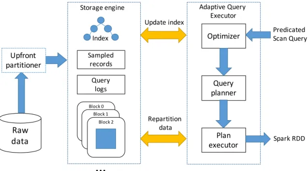
Raw data Optimizer Query planner Plan executor Predicated Scan Query Spark RDD Adaptive Query Executor Storage engine Upfront partitioner Update index Repartition data IndexFigure 3 shows the overall architecture of Amoeba. The three key components of Amoeba storage system are as follows:
(i) Upfront partitioner. The upfront partitioner partitions a dataset into blocks and spreads them throughout a block-based file system. The blocks are created based on attributes in the dataset, without requiring a query workload. As a result, users immediately get improved performance on ad-hoc workloads.
(ii) Storage Engine. The storage engine builds on top of a block-based storage system to store tables. Each table represents a dataset loaded using the upfront partitioner. The table contains an index file which stores the partitioning tree used to partition the dataset and the partitioned dataset as a collection of data blocks. In addition, we also store a query log containing the most recent queries that accessed the dataset and a sample of the dataset whose use is described later.
(iii) Adaptive Query Executor. The adaptive query executor takes queries in the form of a predicated scan and returns back the matching tuples. Since Amoeba internally stores the data partitioned by the partition tree, it is able to skip many data blocks while answering queries. The query first goes to the optimizer. When the data blocks accessed by the query are not perfectly partitioned, the optimizer considers repartitioning some or all of the accessed data blocks, as they are accessed by the query and using the query predicates as cut-points. We use a cost model to evaluate the expected cost and benefit of repartitioning. Due to de-clustering, we end up performing random I/Os for each data block. This is ok, large block sizes in distributed file systems [35] combined with fast network speeds lead to remote reads being almost as fast as local reads (See Appendix A). We sacrifice some data locality in order to quickly locate the relevant portions of the data on each machine in a distributed setting.
The Amoeba storage system is self-tuning , lightweight (both in terms of the up-front and repartitioning costs), and does not increase the storage space requirements. In the rest of the thesis, we focus on building an efficient predicate-based data access system. Future work will look at developing query processing algorithms (e.g., join algorithms), on top of this system.
Chapter 4
Upfront Data Partitioning
A distributed storage system, such as HDFS, subdivides a dataset into smaller chunks, called blocks. Blocks are created based on size, such that each block except the last is of B bytes (usually 64MB) and gets independently replicated on R machines, where R is the number of replicas (usually 3). The upload happens in parallel, however it is expensive and involves writing out R copies of the dataset to disk across the cluster. The upfront data partitioning pipeline exploits this block structure to create blocks based on attributes, i.e., it splits the data by attributes rather than partitioning with-out regard to the values in each block. This is similar to content-based chunking [36] and feature-based blocking [7], however our approach does not depend on a query workload. The key idea is to integrate attribute-based partitioning with data block-ing, i.e., splitting a dataset into data blocks, in the underlying storage system using a partitioning tree. This helps Amoeba achieve improved query performance on almost all ad-hoc queries, compared to standard full scans, without having any information about the query workload. This partitioning also serves as a good starting point for the adaptive data repartitioner to improve upon, as discussed in Chapter 5.
We first present the key ideas used in the upfront partitioner. Then, we describe our partitioning algorithm to come up with a partitioning tree for a given dataset.
4.1
Key Ideas
(1) Balanced Binary Tree. We represent the partitioning tree as a balanced binary tree, i.e., we successively partition the dataset into two until we reach the minimum
partition size. Each node in the tree is represented as Ap where A is attribute being
partitioned on and p is the cut-point. All tuples with A ≤ p go to the left subtree and rest go to the right subtree. The leaf nodes in the tree are buckets, each having a unique identifier and the file name in the underlying file system. This file contains the tuples that satisfy the predicates of all nodes traversing upwards from the bucket to the root of the tree. Note that an attribute can appear in multiple nodes in the tree. Having multiple occurrences of an attribute in the same branch of the tree increases the number of ways the data is partitioned on that attribute.
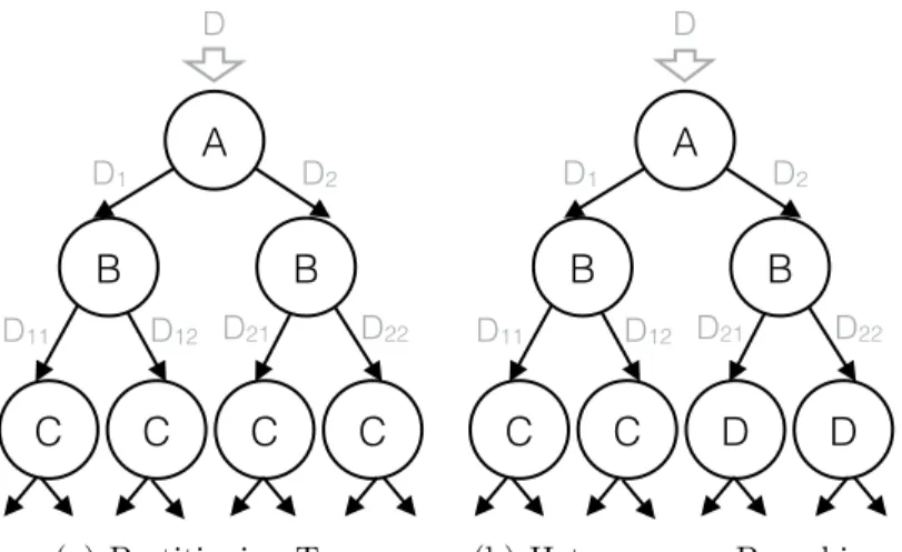
(2) Heterogenous Branching. Figure 4-1(a) shows a partitioning tree analogous to the k-d tree. This tree can only accommodate as many attributes as the depth of the tree. For a dataset size D, minimum partition size P , and n way partitioning over each
attribute, the partitioning tree contains blognDPc attributes. With n = 2, D = 1TB,
and P = 64MB, we can only accommodate 14 attributes in the partitioning tree. However, many real-world schemas have way more attributes. To accommodate more attributes, we introduce heterogeneous branching to partition different branches of the partitioning tree on different attributes. Hence, we sacrifice the best performance on a few attributes to achieve improved performance over more attributes. This is reasonable as without a workload, there is no reason to prefer one attribute over another. Figure 4-1(b) shows a partitioning tree with heterogenous branching. After partitioning on attributes A and B, the left side of the tree partitions on C while the right side partitions on D. Thus, we are now able to accommodate 4 attributes, instead of 3. However, attributes C and D are each partitioned on 50% of the data. As a result, ad-hoc queries would now gain partially but over all the four attributes, which makes the partitioning robust.
The number of attributes in the partitioning tree, with c as the minimum fraction of the data partitioned by each attribute and r as the number of replicas, is given
as 1c · blognDPc. With n = 2, D = 1TB, P = 64MB and c = 50%, the number of
C C C C A B B D1 D2 D11 D D12 D21 D22 C C D D A B B D1 D2 D11 D D12 D21 D22 C D E F Replicate A B D1 D2 D11 D D12 D21 D22
(a) Partitioning Tree.
C C C C A B B D1 D2 D11 D D12 D21 D22 C C D D A B B D1 D2 D11 D D12 D21 D22 C D E F Replicate A B D1 D2 D11 D D12 D21 D22 (b) Heterogenous Branching. Figure 4-1: Partitioning Techniques.
be partitioned increases with the dataset size. This shows that with larger dataset sizes, upfront partitioning is even more useful for quickly finding the relevant portions of the data.
(3) Hedging Our Bets. We define the allocation of an attribute i at each node j in the
tree as the number of ways the node partitions that attribute (nij) times the fraction
of the dataset this partitioning is applied to (cij), i.e., the total allocation of attribute
i is given as:
Allocationi = Σcij · nij
Allocation as defined above gives the average fanout of an attribute. For example, in Figure 4-1(b), attribute B has an allocation of (2 ∗ 0.5 + 2 ∗ 0.5) = 2, while attribute C has an allocation of (2 ∗ 0.25 + 2 ∗ 0.25) = 1. If we distribute the allocation equally among all attributes, then the maximum per-attribute allocation for |A| attributes
and b buckets is given as b1/|A|. For example, if there are 8 buckets, and 3 attributes,
the allocation (average fanout) per attribute is 81/3= 2.
The key intuition behind our upfront partitioning algorithm is to compute this maximum per-attribute allocation, and then place attributes in the partitioning tree so as to approximate this ideal allocation.
(4) Handling skew and correlations efficiently. Real world datasets are often skewed (e.g., recent sales, holiday season shopping, etc.), and have attributes that are
cor-attributes={A,B,C,D} buckets = 8 depth = 3 alloc[A] = 1.189 alloc[B] = 1.189 alloc[C] = 1.189 alloc[D] = 1.189 alloc[A] = -0.811 alloc[B] = 1.189 alloc[C] = 1.189 alloc[D] = 1.189 alloc[A] = -0.811 alloc[B] = 0.189 alloc[C] = 1.189 alloc[D] = 1.189 alloc[A] = -0.811 alloc[B] = 0.189 alloc[C] = 0.189 alloc[D] = 1.189 alloc[A] = -0.811 alloc[B] = 0.189 alloc[C] = 0.189 alloc[D] = 0.689 alloc[A] = -0.811 alloc[B] = 0.189 alloc[C] = 0.189 alloc[D] = 0.189 alloc[A] = -0.811 alloc[B] = -0.311 alloc[C] = 0.189 alloc[D] = 0.189 alloc[A] = -0.811 alloc[B] = -0.311 alloc[C] = 0.189 alloc[D] = -0.311
(i) (ii) (iii) (iv) (v) (vi) (vii)
B C A B A A D4 D4 B5 D6 B7 C3 A5 A2 D4 B5 D6 B7 C3 A5 A2 A2 B5 D6 B7 C3 A5 B7 B7 B5 D6 A2 C3 A5
Swap D4 Swap D4 Pushdown B7 Rotate A5
A2 B5 D6 C3 A5 B C A D D B D B C A D D B B C A D D B C A D B7 B7
Figure 4-2: Upfront Partitioning Algorithm Example.
related (e.g., state and zipcode). As a result, if we uniformly partition by attribute value, some branches of the partitioning tree could have much more data than others, resulting in unbalanced final partitions. We would then lose the benefit of partition-ing due to either very small or very large partitions. To illustrate, consider a skewed
dataset D1 = {1, 1, 1, 2, 2, 2, 3, 4, 5, 6, 7, 8} and two partitionings, one based on the
domain values and the other on the median value.
Pdomain(D1) = [{1, 1, 1, 2, 2, 2}, {3, 4}, {5, 6}, {7, 8}]
Pmedian(D1) = [{1, 1, 1}, {2, 2, 2}, {3, 4, 5}, {6, 7, 8}]
We can see that Pdomain(D1) is clearly unbalanced whereas Pmedian(D1) produces
bal-anced partitions. Likewise, to illustrate the effect of correlations, consider a dataset
D2 with two attributes country name and salary :
D2(country, salary) ={(X, $25), (X, $40), (X, $60), (X, $80), (Y, $600),
(Y, $700), (Y, $850), (Y, $950)}
Pdomain(D2) =[{(X, $25), (X, $40), (X, $60), (X, $80)}, {(Y, $600),
(Y, $700), (Y, $850), (Y, $950)}]
Pmedian(D2) =[{(X, $25), (X, $40)}, {(X, $60), (X, $80)}, {(Y, $600),
(Y, $700)}, {(Y, $850), (Y, $950)}]
Partitioning D2 on country followed by salary results in only two partitions when
splitting the salary over its domain (0 through 1000). This is because the salary distributions are correlated with the country. However, we get all four partitions when using the medians successively on each node.
Algorithm 1: UpfrontPartitioning
Input : Attribute[] attributes, Int datasetSize, Int partitionSize Output: Tree partitioningTree
1 numBuckets ← datasetSize / partitionSize;
2 depth ← log2(numBuckets);
3 foreach a in attributes do
4 allocation[a] ← nthroot(numBuckets, size(attributes));
5 root ← CreateNode();
6 CreateTree(root, depth, allocation);
7 return root;
Amoeba avoids this problem by performing a breadth-first traversal while con-structing the partitioning tree. At each node, we place the attribute which has the maximum allocation remaining. Once the attribute is chosen, we sort the data ar-riving at the node on the attribute and choose the median as the pivot. We split the data on the pivot and proceed to assign (attribute, pivot) for the left and right child nodes. Finding the median in the data handles skew and correlation between attributes, thereby ensuring that child nodes get equal portions of data. This leads to balanced partitions in the end. In order to find the medians efficiently, we first make one pass over the data to construct a sample and then find the median at each node using the sample. We refer to Chapter 6 for more details on implementation.
4.2
Upfront Partitioning Algorithm
We now describe our upfront partitioning algorithm. The goal of the algorithm is to generate a partitioning tree, which balances the benefit of partitioning across all attributes in the dataset. This means that same selectivity predicates on any two attributes X and Y should have similar speed-ups, compared to scanning the entire dataset. Notice that this is different from a k-d tree [37] which typically partitions the space by considering the attributes in a round robin fashion, until the smallest partition size is reached. Before we describe the algorithm, let us first look at the key ideas in our upfront partitioning algorithm.
Algorithm 2: CreateTree
Input : Tree tree, Int depth, Int[] allocation
1 Queue nodeQueue ← {tree.root};
2 while nodeQueue.size > 0 do 3 node ← nodeQueue.pollFirst(); 4 if depth > 0 then 5 node.attr ← leastAllocated(allocation); 6 node.value ← findMedian(node.attr ); 7 node.left ← CreateNode(); 8 node.right ← CreateNode();
9 allocation[node.attr] -= 2.0/2maxDepth - depth;
10 nodeQueue.add(node.left);
11 nodeQueue.add(node.right);
12 depth -=1;
13 else
14 node ← newBucket ();
of attributes, the dataset size, and the smallest partition size1 and produces the
partitioning tree. The algorithm computes the ideal allocation for each attribute and then calls createTree on the root node. Note that we could also consider relative weights of attributes when computing the ideal allocation for each attribute, in case some attributes are more likely to be queried than others. Algorithm 2 shows the createTree function. It performs a breadth-first traversal and assigns an attribute to each node. The attribute to be assigned is given by the function leastAllocated, which returns the attribute which has the highest allocation remaining. If two or more attributes have the same highest allocation remaining, we randomly choose among the ones that have occurred the least number of times in the path from the node to the root. findMedian returns the median of the attribute assigned to this node. This is done by finding the median in the sampled data which comes to this branch. The algorithm starts with an allocation of 2 for the root node, since we are partitioning the entire dataset into two partitions. Each time we go to the left or the right subtree, we reduce the data we operate on by half. Once an attribute is assigned to a node, we subtract from the overall allocation of the attribute (Line 9). The algorithm creates a leaf-level bucket in case we reach the maximum depth (Line 14).
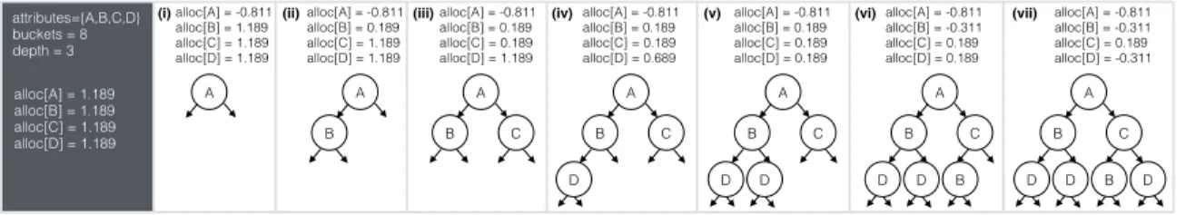
Figure 4-2 illustrates the steps when assigning attributes in a partitioning tree over 4 attributes and 8 buckets (dataset size = 8 ∗ 64 = 512MB) and the allocation remaining per attribute in each step. The algorithm starts in Step (i) with the root node and performs a breadth-first traversal. Once attribute A is assigned in Step (i), it has the least allocation remaining (in fact, we have used up all the allocation for attribute A) and it is excluded from the possible options in Step (ii). We continue placing attributes with the minimum allocation even after all four attributes have been placed once in Step (iv). At the end of Step (v), attributes B, C, and D have the same allocation remaining. For the next nodes in Steps (vi) and (vii), since C already occurs on the path from the nodes to the root, we randomly choose between B and D.
Chapter 5
Adaptive Repartitioning
In the previous chapter, we described an algorithm to partition a dataset on several (or all) attributes, without knowing the query workload. However, as users begin to query the dataset, it is beneficial to improve the partitioning based on the observed queries. As in most online algorithms, we assume that the queries seen thus far are indicative of the queries to come. Amoeba does this by doing transformations on the partitioning tree based on the observed data access patterns. The key features of the adaptive repartitioning module of Amoeba are:
• Piggybacked, meaning it interleaves with query processing and only accesses the data which is read by input query, i.e., we do not access data that is not read by queries during re-partitioning. This has two benefits: (i) we never spend any effort in re-partitioning data that will not be touched by any query, and (ii) query processing and re-partitioning modules share the scan thereby reducing the cost of re-partitioning.
• Transparent, as the users do not have to worry about making the repartitioning decisions and their queries remain unchanged with new access methods.
• Eventually convergent, meaning it converges to a final partitioning if a fixed workload is repeated over and over again.
• Lightweight, as it does not penalize any query with high repartitioning costs: it distributes the costs over several queries.
• Balances between adaptivity and robustness, meaning the system tries to stabi-lize newly made repartitioning decisions as well as expiring older decisions. In the rest of this chapter, we first describe our workload monitor and the cost
model to estimate the cost of a query over a given partitioning tree. Then, we
introduce three basic transformations used to transform a given partitioning tree. We describe a bottom-up algorithm to consider all possible alternatives generated from the transformation rules for inserting a single predicate. Finally, we discuss how to handle multi-predicate queries.
5.1
Workload Monitor and Cost Model
Amoeba maintains a history of the queries seen by the system. We call this the query window denoted by W . Each incoming query gets added into the query window as < T, q > where T is the current timestamp and q is the query. We do not directly restrict the size of the query window, instead we restrict the window to contain only queries that happened in the past X hours. The intuition behind this is that the older queries are stale and are not the representative of the queries to be seen. In all our evaluation, we set W = 4 hours. The cost of a query q over a partitioning tree T is given as:
Cost(T, q) = X
b∈lookup(T ,q)
nb
Where the function lookup(T, q) gives the set of relevant buckets for query q in T . The cost of the query window is the sum of the cost of individual queries. A query being executed may have some of its buckets re-partitioned. The added cost of repartitioning a set of buckets B is given as:
RepartitioningCost(T, q) =X
b∈B
The important parameter to note here is c. c represents the write-multiplier i.e.: how expensive writes are compared to read. Changing c alters the properties of the system: on one end setting c = ∞ makes it imitate a system with no-repartitioning, at the other end setting c = 0 makes it re-partition the data every time it sees benefit.
5.2
Partitioning Tree Transformations
We now describe a set of transformation rules to explore the space of possible plans
when re-partitioning the data. For now, we restrict ourselves to the problem of
exploring alternate trees for a query with a single predicate of the form A ≤ p,
denoted as Ap. Later in 5.4, we discuss how to handle other predicate forms and
adding multiple predicates into the tree.
Given a query with predicate Ap, we attempt to assign Ap to one of the nodes
(partition on A with cutpoint p) in the partitioning tree. Note that we do not have to consider partitioning on any other attribute, i.e., predicates on other attributes would have already been considered when there was a query on that attribute. Our approach is to consider partitioning transformations that are local, i.e., that do not involve rewriting the entire tree. These local transformations are cheaper and amor-tizes the repartitioning effort over several queries. Below, let us first see the three kinds of partitioning transformations that we consider during repartitioning. We will then describe our algorithm for when to apply these transformations in order to im-prove the query performance. Amoeba considers three kinds of basic partitioning transformations:
(1) Swap. This is the primary data-reorganization operator in Amoeba. It replaces
an existing node in the partitioning with the incoming query predicate Ap. As we
repartition only the accessed portions of the data, we consider swapping only those nodes whose left and right children are accessed by the incoming query. Applying swap on an existing node involves reading both sub-branches, and restructuring all
partitions beneath the left subtree to contain data satisfying Ap and the right
sub-tree to contain data that does not satisfy Ap. Swaps can happen between different
attributes (Figure 5-1(a)), in which case both branches are completely rewritten in the new tree. Swaps can also happen between two predicates of the same attribute
(Figure 5-1(b)), in which case the data moves from one branch to the other. X Ap Ap' Ap X Ap Ap Ap X X Ap' Z Ap X Y X Ap X Y Ap' Q[Ap] Q[Ap] Q[Ap] Q[Ap]
(a) Different Attribute Swap
X Ap Ap' Ap X Ap Ap Ap X X Ap' Z Ap X Y X Ap X Y Ap' Q[Ap] Q[Ap] Q[Ap] Q[Ap]
(b) Same Attribute Swap Figure 5-1: Node swap in the partitioning tree.
For example, if predicate Ap0 is ≤ 10 and predicate Ap is ≤ 5, then data moves
from left branch to right branch in the Figure 5-1(b), i.e., the left branch is com-pletely rewritten while the right branch just has new data appended. Swaps serve the dual purpose of un-partitioning an existing (less accessed) attribute while refining on another (more accessed) attribute. Since both the swap attributes as well as their predicates are driven by the incoming queries, they reduce the access times for the incoming query predicates. Finally, note that it is cheaper to apply swaps at lower levels in the partitioning tree since less data is rewritten. Applying them at higher levels of the tree results in a much higher cost.
(2) Pushup. This transformation is used to push a predicate as high up the tree as possible. This can be done when both the left and the right child of a node contain the incoming predicate, as a result of a previous swap, as shown in Figure 5-3. Notice that this is a logical partitioning tree transformation, i.e., it only involves rearranging
the internal nodes without any modification of the contents of leaf nodes1.
We check for a pushup transformation every time we perform a swap transformation. The idea is to move important predicates (ones that have recently or frequently ap-peared in the query sequence) progressively up the partitioning tree, from the leaves right up to the root. This makes such important predicates less likely to be swapped immediately, i.e., the tree is still robust, because swapping a node higher in the par-titioning tree is much more expensive. Another advantage of node pushup is that it causes a churn of the attributes assigned to higher nodes in the upfront partitioning. When such a dormant node is pushed down, subsequent predicates can swap them in a more incremental fashion, affecting fewer branches. Overall, node pushup allows Amoeba to naturally cause less important attributes to be repartitioned more fre-quently, thereby striking a balance between adaptivity and robustness. Note that if
1In this case, the physical transformation, i.e. swap, must have happened in one of the child
attributes={A,B,C,D} buckets = 8 depth = 3 alloc[A] = 1.189 alloc[B] = 1.189 alloc[C] = 1.189 alloc[D] = 1.189 alloc[A] = -0.811 alloc[B] = 1.189 alloc[C] = 1.189 alloc[D] = 1.189 alloc[A] = -0.811 alloc[B] = 0.189 alloc[C] = 1.189 alloc[D] = 1.189 alloc[A] = -0.811 alloc[B] = 0.189 alloc[C] = 0.189 alloc[D] = 1.189 alloc[A] = -0.811 alloc[B] = 0.189 alloc[C] = 0.189 alloc[D] = 0.689 alloc[A] = -0.811 alloc[B] = 0.189 alloc[C] = 0.189 alloc[D] = 0.189 alloc[A] = -0.811 alloc[B] = -0.311 alloc[C] = 0.189 alloc[D] = 0.189 alloc[A] = -0.811 alloc[B] = -0.311 alloc[C] = 0.189 alloc[D] = -0.311
(i) (ii) (iii) (iv) (v) (vi) (vii)
B C A B A A D4 D4 B5 D6 B7 C3 A5 A2 D4 B5 D6 B7 C3 A5 A2 A2 B5 D6 B7 C3 A5 B7 B7 B5 D6 A2 C3 A5
Swap D4 Swap D4 Pushdown B7 Rotate A5
A2 B5 D6 C3 A5 B C A D D B D B C A D D B B C A D D B C A D B7 B7
Figure 5-2: Illustrating adaptive partitioning when predicate A2 appears repeatedly.
X Ap Ap' Ap X Ap Ap Ap X X Ap' Z Ap X Y X Ap X Y Ap' Q[Ap] Q[Ap] Q[Ap] Q[Ap]
Figure 5-3: Node pushdown in partitioning tree.
possible, a pushup always happens as there is no cost associated with doing it. (3) Rotate. The rotate transformation rearranges two predicates on the same at-tribute such that more important (recently accessed or frequently appearing in the query sequence) predicate appears higher up in the partitioning tree. Figure 5-4 shows
a rotate transformation involving predicates p and p0 on attribute A. The goal here
is to churn the partitioning tree such that predicates on less important attributes are likely to be replaced first. Similar to the pushup transformation, rotate is a logical transformation, i.e., it only rearranges the internal nodes of the partitioning tree and always happens if possible.
X Ap Ap' Ap X Ap Ap Ap X X Ap' Z Ap X Y X Ap Y Z Ap' Q[Ap] Q[Ap] Q[Ap] Q[Ap]
Figure 5-4: Node rotation in partitioning tree.
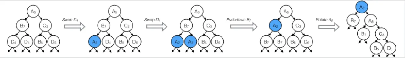
These three partitioning tree transformations can be further combined to capture a fairly general set of repartitioning scenarios. Figure 5-2 shows how starting from
an initial partitioning tree, we first swap nodes D4 with incoming predicate A2 at the
lower level. Then, we pushup A2 one level above and finally rotate with nodes A5
and C3.
The upfront partitioning algorithm generates a partitioning tree which is fairly balanced, i.e., all the leaf nodes get almost same number of tuples. Swapping nodes based on predicates from incoming queries may lead to some leaves having more tuples compared to the rest. This is not a problem as our cost model ensures that the skew is actually beneficial if it arises. For example, if many queries access A ≤ 0.75, where
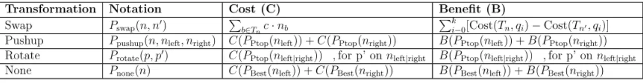
Transformation Notation Cost (C) Benefit (B)
Swap Pswap(n, n0)
P b∈Tnc · nb
Pk
i−0[Cost(Tn, qi) − Cost(Tn0, qi)] Pushup Ppushup(n, nleft, nright) C(PPtop(nleft)) + C(PPtop(nright)) B(PPtop(nleft)) + B(PPtop(nright)) Rotate Protate(p, p0) C(PPtop(nleft|right)) , for p’ on nleft|right B(PPtop(nleft|right)) , for p’ on nleft|right None Pnone(n) C(PBest(nleft)) + C(PBest(nright)) B(PBest(nleft)) + B(PBest(nright)) Table 5.1: The cost and benefit estimates for different partitioning tree transforma-tions.
A is uniformly distributed (0, 1), it is beneficial to add this node into the tree even though it might lead to a skew. In the next section, we describe how we generate alternate partitioning trees using these transformations.
5.3
Divide-And-Conquer Repartitioning
Given a query with predicate Ap and a partitioning tree T , there are many different
combinations of transformations that need to be considered. Consider for example a simple 7-node tree, consisting of a root node X with two children Y and Z. Each of Y and Z have two leaf nodes below them. Assuming all the leaf nodes are accessed,
the set of alternatives to be considered are: (i) Swap Y with Ap; (ii) Swap Z with
Ap; (iii) Swap both Y and Z, followed by pushup; (iv) Swap X with Ap; and (v) Do
nothing.
We propose a bottom-up approach to explore the space of all alternate
reparti-tioning trees. Observe that the data access costs over a partireparti-tioning tree Tn, rooted
at node n, could be broken down into the access costs over its subtrees, i.e.,
Cost(Tn, qi) = Cost(Tnlef t, qi) + Cost(Tnright, qi)
Where, Tnlef t and Tnright are subtrees rooted respectively at the left and the right
child of n. Thus, finding the best partitioning tree can be broken down into recursively finding the best left and right subtrees at each level, and considering parent node transformations only on top of the best child subtrees. For each transformation, we consider the benefit and cost of that transformation and pick the one which has the best benefit-to-cost ratio. Table 5.1 shows the cost and benefit estimates for different
transformations. For the swap transformation, denoted as Pswap(n, n0), we need to
Algorithm 3: getSubtreePlan Input : Node node, Predicate pred Output: Plan transformPlan
1 if isLeaf(node) then
2 return Pnone(node);
3 else
4 if isLeftRelevant(node,pred ) then
5 leftPlan ← getSubtreePlan(node.lChild, pred );
6 if isRightRelevant(node,pred ) then
7 rightPlan ← getSubtreePlan(node.rChild, pred );
/* consider swap */
8 if leftPlan.fullyAccessed and rightPlan.fullyAccessed then
9 currentCost ← Pi Cost(node,qi);
10 whatIfNode ← clone(node);
11 whatIfNode.predicate ← newPred;
12 swapNode(node, whatIfNode);
13 newCost ← Pi Cost(whatIfNode,qi);
14 benefit = currentCost - newCost;
15 if benefit > 0 then
16 updatePlanIfBetter(node, Pswap(node,whatIfNode));
/* consider pushup */
17 if leftPlan.ptop and rightPlan.ptop then
18 updatePlanIfBetter(node, Ppushup(node, node.lChild, node.rChild));
/* consider rotate */
19 if node.attribute == predicate.attribute then
20 if leftPlan.ptop then
21 updatePlanIfBetter(node, Protate(node, node.lChild));
22 if rightPlan.ptop then
23 updatePlanIfBetter(node, Protate(node, node.rChild));
/* consider doing nothing */
24 updatePlanIfBetter(node, Pnone(node));
25 return node.plan;
as Pswap(n, n0) and Ppushup(n, nleft, nright) respectively, inherit the costs from children
subtrees. We also consider applying none of the transformations at a given node,
denoted as Pnone(n). This divide-and-conquer approach helps to significantly reduce
the candidate set of modified partitioning trees.
algorithm uses a divide-and-conquer approach to find the best plan for the given predicate by recursively finding the best plan for each subtree, until we reach the leaf. If the node is a leaf, we return a do-nothing plan (Lines 1-2). If not, we first check if the left subtree is accessed, if yes we recursively call getSubtreePlan to find the best plan for the left subtree (Lines 4-6). Similarly for the right subtree. Once we have the best plans for the left and right subtree, we first consider swap rule (Lines 10—19). We only consider swapping if both the subtrees are fully accessed. Otherwise, we will need to access additional data in order to create new partitioning. We perform a what-if analysis to analyze the plan produced by the swap transfor-mation. This is done by replacing the current node with a hypothetical node having the incoming query predicate. We then recalculate the new bucket counts at the leaf level of this new tree using the sample. We now estimate the total query cost with the hypothetical node present. In case the what-if node reduces the query costs, i.e., it has benefits, we update the transformation plan of the current node. The update method (updatePlanIfBetter) checks whether the benefit-cost ratio of the new plan is greater than that of the best plan so-far. If so, we update the best plan. The benefit-cost ratio is used to compare the alternative plans.
Next we check whether a pushup transformation is possible (Lines 21–23). plan.ptop indicates if the plan results in the predicate p being at the root of the subtree. A pushup transformation is possible only when both the child nodes have their root
as Ap. Since pushup is only a logical transformation, we do not need to perform a
what-if analysis. Instead, we simply check whether the pushdown results in better benefit-cost ratio in the updatePlanIfBetter method. Then, we consider rotating the node by bringing either the left or the right child up (Lines 24–31). Again, this is a logical transformation and therefore we only check the benefit-cost ratio. Finally, we check whether no transformation is needed, i.e., we simply inherit the transfor-mations of the child nodes (Lines 32). The algorithm finally returns the best plan in Line 33.
A plan contains action taken at the node, ptop to indicate if after the plan is
applied Ap is the root, f ullyAccessed to indicate if the entire subtree is accessed
and pointers to the plan for the left and right child nodes. For the sake of brevity, Algorithm 3 does not explicitly show the update of these attributes. The algorithm
Algorithm 4: getBestPlan
Input : Tree tree, Predicate[] predicates
1 while predicates 6= φ do
2 prevPlan ← tree.plan;
3 foreach p in predicates do
4 Plan newPlan ← getSubtreePlan(tree.root, p);
5 updatePlan(tree.root, newPlan);
6 if tree.plan 6= prevPlan then
7 remove from predicates the newly inserted predicate;
8 else
9 break;
10 return tree.plan;
has a runtime complexity of O(QN logN ) where N is the number of nodes in the tree and Q is the number of queries in the query window.
5.4
Handling Multiple Predicates
So far we assumed that a predicate is always of the form A ≤ p. It gets inserted in
the tree as Ap and on insertion, only the leaf nodes on the left side of the tree are
accessed. A > p is also inserted as Ap with the right side of the tree being accessed.
For A ≥ p and A < p, let p0 be p − δ where δ is the smallest change for that type.
We insert Ap0 into the tree. A = p is treated as combination of A ≤ p and A > p0.
Now lets consider queries with multiple predicates. Consider a simple query with
two predicate Ap and Ap2. The brute force approach is to consider choosing a set
of accessed non-terminal nodes to be replaced by Ap and then for every such choice,
choose a subset of remaining nodes to be replaced by Ap2. Thus, the number of choices
grows exponentially with the number of predicates. Amoeba uses a greedy approach to work around this exponential complexity, as described in Algorithm 4. For each predicate in the query, we try to insert the predicate into the tree. We find the best
plan for that predicate by calling getSubtreeP lan(root, pi) for the ithpredicate (Lines
3-6). We take the best among the best plans obtained for different predicates and remove the corresponding predicate from the predicate set. We then try to insert the remaining predicates into the best plan obtained so far. The algorithm stops when
either all predicates have been inserted or when the tree stops changing (Lines 1 and
10). getBestP lan adds a multiplicative complexity of O(|P |2) where P is the set of
Chapter 6
Implementation
We now describe our implementation of Amoeba on top of HDFS and Apache Spark. Notice that our ideas could be implemented on any other block-based distributed storage system. The Amoeba storage system has more than 12, 000 lines of code and it comprises of two modules: (i) a robust partitioning module that parses data and writes out the initial partitions; and (ii) a query executor module performing the distributed adaptive repartitioning.
6.1
Initial Robust Partitioning
This module takes in the raw input files (e.g., CSV) and partitions them across all attributes. For this, it first builds the robust partitioning tree and then creates the data blocks based on the partitioning tree.
Tree Construction. Recall that our robust partitioning algorithm needs to find the median value of the partitioning attribute at each node of the tree. As finding successive medians on the entire dataset is expensive, we instead employ a sample of the input to estimate the median. We use block-level sampling to generate a random sample of the input.
Amoeba uses a lazy parser to parse the input sample data lazily. The parser detects: the record boundaries, the attribute boundaries inside a record and the data types. Each value in the record is actually parsed only when it is accessed, i.e., lazily. While Amoeba partitions on all attributes by default, developers can also specify
particular subsets of the attributes to partition on, in case they have some knowledge of the query workload. In such a situation, only the partitioned attributes need to be parsed. Finally, the lazy parser avoids copying costs by returning tuples as views on the input byte buffer. The only time copying happens when the tuple is written to an output byte buffer.
The sampled records and set of attributes are fed to the tree builder (Algorithm 2), which produces the partitioning tree as the output. The tree builder successively sorts the sample on different attributes in order to find the median at different nodes in the tree. However, as each sort happens on a different portion of the sample, we sort on different views of the same underlying data, i.e., the samples are not copied each time they are sorted. When constructing the partitioning tree on a cluster of machines, we collect the samples on each machine independently and in parallel. Later, we combine the samples (via HDFS) and run the tree builder on a single machine to produce a single partitioning tree across the entire dataset. The index is serialized and stored as a file on HDFS.
Data Blocking. The second phase takes the partitioning tree and the input files as input and creates the data blocks. During this phase, we scan the input files, for each tuple we use the partitioning tree to find the leaf node it lands in. We use a buffered blocker to collect the tuples belonging to each partition(leaf node) separately and buffer them before flushing to the underlying file system, i.e., HDFS in our case. Our current implementation creates a different HDFS file for each partition in the dataset. However, future work could also integrate Amoeba deeply within HDFS. Given that we do not assume any workload knowledge, Amoeba simply de-clusters the partitioned blocks randomly across the cluster of machines, i.e., we use the default random data placement policy of HDFS. This is reasonable because fetching relevant data across the network is fine if we can skip more expensive disk reads, as noted in the introduction.
Amoeba runs the loading and partitioning in parallel on each machine, using the same partitioning tree (made available to all machines via HDFS). We employ partition-level distributed exclusive locks (via Zookeeper) to ensure that buffered writers on different machines don’t write to the same file at the same time. With the current main memory and CPU capacities, having a file per partition (number of
partitions in the order of ten thousand) does not lead to any observable slowdown [38].
6.2
Query Execution
There are two main parts involved in query execution: (i) create an execution plan which may involve re-partitioning some or all the of the data that is being accessed by the query, and (ii) actually execute the plan.
Optimizer. Queries submitted to Amoeba first go to the optimizer. The optimizer is responsible for generating an execution plan for the given query. It reads the current tree file from the HDFS and uses Algorithm 4 to check if it is feasible to improve the current partitioning tree. Note that while creating the plan, we also end up filtering out partitions which do not match any of the query predicates. For example, if there
is a node A5 in the tree and one of the predicates in the query is A ≤ 4, then we don’t
have to scan any of the partitions in right subtree of the node. The plan returned is used to create a new index tree and write it out to HDFS. From the plan, we now get two set of buckets: 1) buckets that will just be scanned, and 2) buckets that will be re-partitioned to generate a new set of buckets.
Plan Executor. Amoeba uses Apache Spark for executing the queries. We con-struct a Spark job from the plan returned by the optimizer. We split the each of the two sets of buckets into smaller sets called tasks. A task contains a set of buckets such that the sum of the sizes of the buckets is not more than 4GB. Each task reads the blocks from HDFS in bulk and iterates over the tuples in main-memory. Tasks created from set 1 run with a scan iterator which simply reads a tuple at a time from the buckets and returns the tuple if it matches the predicates in the query.
Tasks created from set 2 run with a distributed repartitioning iterator. The it-erator reads the tree from HDFS. For each tuple, the itit-erator looks up in the new partitioning tree to find its new partition id in addition to checking if it matches the query predicates. It then re-clusters the data in main-memory according to the new partitioning tree. Once the buffers are filled, the repartitioner flushes the new parti-tions into physical files on HDFS. When the optimizer decides to repartition a large subtree, the repartitioning work may end up being distributed across several tasks. As a result, the workers need to coordinate while flushing the new partitions, i.e., so
that writes are done atomically. Again, we employ partition-level distributed exclu-sive locks (via Zookeeper) for this synchronization. As a result of this synchronized writing, each partition resides in a single file across the cluster.
Tasks are executed independently by the Spark job manager across the cluster of machines and the result is exposed to the user as a Spark RDD. The user can use these RDDs to do more analysis using the standard Spark APIs, e.g., run an aggregation.
Chapter 7
Discussion
In this chapter we discuss briefly ideas on how to improve the system to get better performance.
7.1
Leveraging Replication
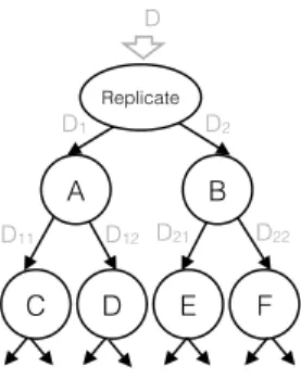
Distributed storage systems replicate data for fault-tolerance, e.g., 3x replication in HDFS. Such replication mechanisms first partition the dataset into blocks and then replicate each block multiple times. Instead, we can first replicate the entire dataset and then partition each replica using a different partitioning tree.
C C C C A B B D1 D2 D11 D D12 D21 D22 C C D D A B B D1 D2 D11 D D12 D21 D22 C D E F Replicate A B D1 D2 D11 D D12 D21 D22
Figure 7-1: Heterogenous Replication.
For example, attributes {A, C, D} and {B, E, F } for the two replicas as in Fig-ure 7.1. While the system is still fault-tolerant (same replication), recovery becomes slower because we need to read several or all replica blocks in case of a block failure. Essentially, we sacrifice fast recovery time for improved ad-hoc query performance.
To recap, the number of attributes in the partitioning tree, with a dataset size D, minimum partition size P , n way partitioning over each attribute, c as the minimum
fraction of the data partitioned by each attribute, is given as a = 1c· blognDPc. Having
r replicas allows us to have a ∗ r number of attributes, with a attributes per replica or increase the n for each attribute. Both these lead to improved query performance due to greater partition pruning. Currently the system just splits the attribute set into disjoint equals sets of attributes and builds a partitioning tree independently on each set. There are interesting questions like can we group together attributes in a non-random way so that cluster attributes accessed together, how to adapt across partition trees which we plan to explore as future work.
7.2
Handling Joins
In order to accelerate join performance, distributed database system tend to do
co-partitioning. Hadoop++[39] and CoHadoop [40] proposed this scheme of
co-partitioning datasets in HDFS to speed up joins.
Co-partitioning can be achieved in Amoeba as well. The user can reserve the d top levels in the partitioning tree for the join attribute on which he/she wants to
co-partition. This creates 2d partitions of the join attribute’s domain. The adaptive
query executor would incrementally re-partition to improve query performance based on the filter predicates but it would not touch the topmost d levels which have been reserved for co-partitioning.
Finally, the dataset may have multiple join attributes, each of which joins to different datasets. Two tables can be partitioned, however a table can’t be co-partitioned against multiple tables on different attributes. The default approach used by systems today is to shuffle join. Shuffle join is much more expensive compared to co-partitioned join as it requires a full network shuffle of the dataset. In Amoeba, since the dataset is partitioned partially (as in not fully co-partitioned), it would be possible to treat joins as a first class query and we could consider adaptively improving the partitioning on the join attribute incrementally as well. It would converge on to fully co-partitioned layout if only one join is frequently accessed. We plan to explore this in the future.
Chapter 8
Evaluation
In this chapter, we report the experimental results on the Amoeba storage system. The experiments are divided into three sub-sections: (i) we examine the benefits and overheads of upfront data partitioning and compare it against a standard space partitioning tree, (ii) we study the behaviour of the adaptive repartitioning under different workload patters via micro benchmarks and (iii) we finally validate the Amoeba system on a real world workload from a local startup company.
Setup. Our testbed consists of a cluster of 10 nodes. Each node has 32 2.07 GHz Xeon cores, running on Ubuntu 12.04, 256 GB main-memory, and 11 TB of disk storage. We generate the dataset in parallel on each node, so all data loading into HDFS happens in parallel. The Amoeba storage system runs on top of current stable Hadoop 2.6.0 and uses Zookeeper 3.4.6 for synchronization. We run queries using Spark 1.3.1, with Spark programs running on Java 7. All experiments are run with cold caches.
8.1
Upfront Partitioning Performance
We now study the impact of doing upfront partitioning. We analyze three aspects: the benefit of doing upfront data partitioning, the added overhead as a result of doing upfront partitioning and finally how it matches up against k-d trees[37] which is a standard space partitioning tree.
The table contains approximately 6 billion rows and 760 GB in size. The table has
16 columns. We use the TPC-H data generator to generate 1/10th of the data on
each machine, hence the data is uniformly distributed across all the machines. After the upfront partitioning is completed, the data resides in HDFS 3-way replicated, occupying 2.3 TB of space.
Attribute Full Scan Robust Partitioning
Robust Partitioning (per-replica)
Ideal Improvement Improvement (per-replica) orderkey 1500 877.228 717.568 75 0.415181333333333 0.521621333333333 partkey 1500 757.293 544.222 75 0.495138 0.637185333333333 suppkey 1500 786.400 385.636 75 0.475733333333333 0.742909333333333 linenumber 1500 793.877 448.731 75 0.470748666666667 0.700846 quantity 1500 764.623 414.005 75 0.490251333333333 0.723996666666667 extendedprice 1500 799.784 251.845 75 0.466810666666667 0.832103333333333 discount 1500 852.987 358.950 75 0.431342 0.7607 tax 1500 794.281 316.465 75 0.470479333333333 0.789023333333333 returnflag 1500 1145.608 1116.729 75 0.236261333333333 0.255514 linestatus 1500 715.728 715.728 75 0.522848 0.522848 shipdate 1500 849.732 484.058 75 0.433512 0.677294666666667 commitdate 1500 838.666 497.604 75 0.440889333333333 0.668264 receiptdate 1500 802.018 475.641 75 0.465321333333333 0.682906 shipinstruct 1500 1039.717 676.373 75 0.306855333333333 0.549084666666667 shipmode 1500 859.939 365.166 75 0.426707333333333 0.756556 0 0.436538622222222 0.654723511111111 T ime (se co n d s) 0 400 800 1200 1600 orderke y partke y supp key linen umb er quantity exten dedp rice disco unt tax retu rnfla g linest atus ship date commi tdat e rece iptd ate ship inst ruct ship mode Full Scan Robust Partitioning Robust Partitioning (per-replica) Ideal
Figure 8-1: Ad-hoc query runtimes for different attributes of TPC-H lineitem.
Ad-hoc Query Processing. We first study ad-hoc query performance. We run
range queries of the following form on all the attributes: SELECT * FROM lineitem
WHERE start < A ≤ end; start and end are chosen randomly in the domain while
ensuring a 5% selectivity. Given that Amoeba distributes the partitioning effort over all attributes, ad-hoc queries are expected to show a benefit right from the beginning. Figure 8-1 shows the results. Two observations stand out: (i) Amoeba (labeled “Robust Partitioning”) bridges the gap between the standard and the ideal runtimes, and (ii) all attributes have similar advantage with Amoeba. Overall, as a result of upfront partitioning we get 44% improvement on an average over full scan versus no partitioning. Figure 8-1 also shows the runtimes for per-replica robust partitioning, i.e., when we use a different partitioning tree for each replica. We can see that per-replica robust partitioning improves the runtimes even further with an average improvement of 65% over full scan. However, note that attributes such as returnflag and linestatus still have the same runtime. This is because these are very low cardinality attributes that cannot be partitioned further. Thus, Amoeba indeed provides improved query performance over ad hoc workloads without being given a workload upfront.
Partitioning overheads. Given that partitioning is an expensive operation in