HAL Id: ird-01905980
https://hal.ird.fr/ird-01905980
Submitted on 26 Oct 2018
HAL is a multi-disciplinary open access archive for the deposit and dissemination of sci-entific research documents, whether they are pub-lished or not. The documents may come from teaching and research institutions in France or abroad, or from public or private research centers.
L’archive ouverte pluridisciplinaire HAL, est destinée au dépôt et à la diffusion de documents scientifiques de niveau recherche, publiés ou non, émanant des établissements d’enseignement et de recherche français ou étrangers, des laboratoires publics ou privés.
Identifying key habitat and spatial patterns of fish
biodiversity in the tropical Brazilian continental shelf
Leandro Eduardo, Thierry Frédou, Alex Souza Lira, Beatrice Padovani
Ferreira, Arnaud Bertrand, Frédéric Ménard, Flávia Lucena Frédou
To cite this version:
Leandro Eduardo, Thierry Frédou, Alex Souza Lira, Beatrice Padovani Ferreira, Arnaud Bertrand, et al.. Identifying key habitat and spatial patterns of fish biodiversity in the tropical Brazilian continental shelf. Continental Shelf Research, Elsevier, 2018, 166, pp.108-118. �10.1016/j.csr.2018.07.002�. �ird-01905980�
DOI: https://doi.org/10.1016/j.csr.2018.07.002
Abstract
Knowledge of the spatial distribution of fish assemblages biodiversity and structure is essential for prioritizing areas of conservation. Here we describe the biodiversity and community structure of demersal fish assemblages and their habitat along the northeast Brazilian coast by combining bottom trawl data and underwater footage. Species composition was estimated by number and weight, while patterns of dominance were obtained based on frequency of occurrence and relative abundance. A total of 7,235 individuals (830 kg), distributed in 24 orders, 49 families and 120 species were collected. Community structure was investigated through clustering analysis and by a non-metric multidimensional scaling technique. Finally, diversity was assessed based on six indices. Four major assemblages were identified, mainly associated with habitat type and depth range. The higher values of richness were found in sand substrate with rocks, coralline formations and sponges (SWCR) habitats, while higher values of diversity were found in habitats located on shallow waters (10–30m). Further, assemblages associated with sponge-reef formations presented the highest values of richness and diversity. In management strategies of conservation, we thus recommend giving special attention to SWCR habitats, mainly those located on depths between 30–60 m. This can be achieved by an offshore expansion of existing MPAs and/or by the creation of new MPAs encompassing those environments.
Keywords: Demersal fish assemblage; Northeast Brazilian coast; Underwater footages;
1. INTRODUCTION
Resource exploitation, climate change, habitat modification, and pollution have led to dramatic modifications in the composition of marine coastal ecosystems (Lotze et al., 2006). These changes are causing rapid loss of populations, species, and entire functional groups (Lotze et al., 2006; Worm et al., 2006). To protect these environments, marine protected areas (MPAs), where fishing and other human activities are restricted or prohibited, have been highly recommended (Dahl et al., 2009). MPAs conserve habitats and marine populations and, by exporting biomass, may also sustain or increase the overall yield of nearby fisheries (Halpern, 2003; Roberts et al., 2001). However, implementing MPAs and prioritizing biodiversity conservation requires human, biophysical and ecological knowledge that is often lacking in some parts of the world (Miloslavich et al., 2011).
Biodiversity has been positively correlated with the structural habitats complexity (Curley et al., 2002). Understanding the relationship between habitat type and fish and describing the spatial distribution of those habitats are therefore essential for informing fisheries management (Curley et al., 2002) and implementing MPAs. Recent advances in collecting and analyzing marine data using cameras and towed video enable direct observation of marine species and their habitats, in more affordable and efficient ways, and in places divers cannot access (Letessier et al., 2013). Even if these approaches may contribute to more effective conservation and management of living marine resources (Mellin et al., 2009) they have not been applied in many marine ecosystems around the world, especially in tropical regions.
Among the Brazilian coastal areas, the northeast coast is the largest (3,000 km) and one of the most densely populated. This region has high biodiversity and includes Ecologically or Biologically Significant Marine Areas (EBSA) (CBD, 2014). Small-scale fisheries (SSF) in the region, directly and indirectly, involve more than 200,000 persons and are responsible for the highest landed volume of the country (Nóbrega et al., 2009). Previous studies focused on fish assemblages in this region, mostly through underwater visual censing (UVC) (e.g. Feitoza et al., 2005; Ferreira et al., 2004) or based on fishery-dependent data (e.g Frédou and Ferreira, 2005; Silva Júnior et al., 2015), provided specific information on the ecology and biology of a variety of species. Nevertheless,
there is a lack of large-scale studies describing biodiversity and assemblage structure in relation to the habitat composition.
Here we describe the biodiversity and community structure of demersal fish assemblages and their habitat along the northeast Brazilian coast by combining bottom trawl data and underwater footages. Overall, this study fills the current gap of knowledge in the area providing a relevant contribution for effective conservation and management of marine resources.
2. MATERIAL AND METHODS 2.1. Study area
The study area (Figure 1) comprises the northeast Brazilian continental shelf, between the states of Rio Grande do Norte and Alagoas (4° - 9°S). This area is located in the eastern part of the northeastern region of the South American Platform, a few degrees north of the southern branch of the South Equatorial Current nearshore bifurcation (Ekau and Knoppers, 1999) and holds a high biodiversity and many priority areas for conservation and sustainable use (CBD, 2014). Within this area, several Marine Protected Areas have been established (e.g. “APA dos Corais”, ‘APA Costa dos Corais’, ‘APA Guadalupe’, ‘APA Santa Cruz’, ‘APA Barra de Mamanguape) (Ferreira and Maida, 2007; Prates et al., 2007). The continental shelf is 40 km width in average with mean depth per latitude ranging from 40 to 80 m and is almost entirely covered by biogenic carbonate sediments (Vital et al., 2010).
2.2. Sampling and sample processing
Data were collected during the Acoustics along the BRAzilian COaSt (ABRACOS) surveys, carried out on 30 August - 20 September 2015 and 9 April – 9 May 2017, on board the French R/V ANTEA. Sampling was conducted using a bottom trawl (body mesh: 40 mm, cod-end mesh: 25mm, entrance dimensions horizontal x vertical: 28 x10 m) at 35 stations (Figure1). Hauls were performed between 10 and 60 m of depth, for about 5 minutes at 3.2 kt. Tow duration was considered as the moment of the arrival of the net on the pre-set depth to the lift-off time, recorded by means of a SCANMAR system. The net geometry has also been monitored using SCANMAR sensors, to give headline height, depth, and distance of wings and doors to ensure the net was fishing correctly. To reduce impacts on benthic habitat and to avoid net damage, the bottom trawl
net was adapted in the second cruise, where bobbins where added to the ground rope. Sampled habitats and geographic areas were similar between surveys, except for the very north oriented coastal area of Rio Grande do Norte which was sampled only during the second cruise. To test for possible changes in gear selectivity among surveys, we compared the size of individuals caught in both surveys. The test was significant, but results did not show important differences (Supplementary Material 1). In addition, we performed a non-parametric permutation procedure ANOSIM (Analysis of Similarity) based on a Bray-Curtis similarity resemblance matrix to test for possible assemblage changes among surveys due to gear adaptation and/or seasonal changes (Clarke et al. 1994). A significant difference was found (R=0.073, p<0.05) but the explained variance was too low for any robust conclusion. Indeed, differences could be due to a survey effect (gear or season) but also to stochastic differences due to unlike sampling locations among surveys. We therefore acknowledge for potential limitation, but we combined both surveys in further analyses to propose a more comprehensive vision of the distribution of fish assemblage.
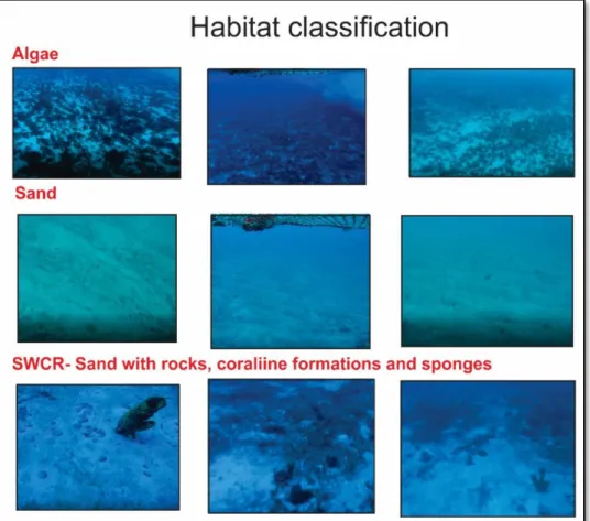
Temperature, salinity, and oxygen profiles were collected for each haul using a CTD (model: SeaBird911). To classify bottom habitat, a video footage was achieved through an underwater camera (GOPRO HERO 3) fitted on the upper part of the mouth of the net. In laboratory, a detailed video analysis was undertaken, where all major habitats were identified. Based on this frame by frame analyses combined with an adaptation of the methodology from Monaco et al. (2012), we were able to consistently identify 3 major types of habitat: (i) Sand with rocks, coralline formations and sponges (SWCR) - primarily sand bottom with 10% or greater distribution of biogenic rocks, corals, calcareous algae and sponges; (ii) Sand - coarse sediment typically found in areas exposed to currents or wave energy; and (iii) Algae - substrates with 10% or greater distribution of any combination of numerous species of leafy red, green or brown algae (Figure 2). After identifying the major habitats, a photo data library with habitats was created to ensure consistency in the video classification process.
Figure 1 - Study area with the bottom-trawl stations (black dots). The position of the Marine Protected Areas (MPA) is indicated (black tick lines and dashed areas).
For each haul, fish were identified, counted, weighed on a motion-compensating scale (to the nearest 0.1 kg), and preserved with a solution of 4% formalin in seawater or by freezing until processing.
2.3. Data analyses
2.3.1. Fish fauna biodiversity and community descriptors
The relative indexes of density and biomass (catch per unit of effort – CPUE) were calculated considering the number of individuals and the weight of fish caught per trawled area (ind.km-2 – kg.km-2). The trawled area was estimated by multiplying the distance covered by the net through the bottom (in m) with the estimated gear mouth opening obtained through the SCANMAR sensors. In six trawls the SCANMAR system was not operative and the average mouth opening (13 m) was utilized.
Figure 2 - Collection of images examples used in habitat classifications along the northeast Brazilian continental shelf (4°- 9°S)
Species composition was estimated by number (%N) and weight (%W). Patterns of dominance were obtained following the methodology of Garcia et al. (2006) and species were classified based on frequency of occurrence (number of occurrences of a species divided by the total number of trawls (x100), %F) and relative abundance (catch per unit effort; %CPUE) per latitude stratum (4°-9°S, intervals of 1°). Species showing %FO > average %FO in each latitude stratum were considered frequent fishes, whereas those with %FO < average %FO were considered rare (Garcia et al., 2006). A similar method was applied to %CPUE, resulting in Higher Abundant (%CPUE > average %CPUE) and Scarce (%CPUE < average %CPUE) categories. Finally, based on these criteria, species were classified in four groups of relative importance (relative importance index): (1) higher abundant and frequent, (2) higher abundant and rare, (3) scarce and frequent and (4) scarce and rare (Garcia et al., 2006). Species were considered dominant when classified within first, second and third categories (Garcia et al., 2006). We also classified the species according to the IUCN Red List categories at the regional level (ICMbio, 2016), which comprises 10 levels: Extinct (EX), Regionally Extinct (RE), Extinct in the Wild (EW), Critically Endangered (CR), Endangered (EN), Vulnerable
(VU), Near Threatened (NT), Least Concern (LC), Data Deficient (DD) and Not Evaluated (NE). The classification criteria, application guidelines, and IUCN Red List methodology on how to apply the Criteria are publically available (IUCN, 2012, 2000).
To investigate the community structure, we performed a Bray-Curtis similarity resemblance matrix, which was used to perform an unweighted arithmetic complete clustering analysis. The non-parametric permutation procedure ANOSIM (Analysis of Similarity) was applied to test for differences among habitat types and depth ranges (intervals of 10 m) (Clarke et al. 1994). To reduce bias in these analyses, species data were log-transformed (log (x + 1)), and infrequent species (those representing <0.1% of abundance) were not considered. As we tested differences among habitats, hauls where the habitat type was classified as unknown were removed from the analysis. The similarity percentage routine (SIMPER) was applied to determine the species contribution to the similarity within a group of sampled sites and the dissimilarity between groups. The set of species that cumulatively contributed to over 70% to the similarity were classed as consolidating, and the set of species contributing to over 70% of dissimilarity between groups were classified as discriminating (Gregory et al., 2016).
Diversity was assessed based on six indices calculated for each haul and by assemblages identified in cluster analyses (Table 1). Diversity indexes were chosen according to the expected complementarity of their conceptual and statistical properties, aiming to access the richness, rarity, commonness and taxonomic distance between species of the community studied (Magurran, 2004; Gaertner et al., 2005; Farriols et al., 2017). The diversities measures Hill’s N1, Hill’s N2 and Pielou’s evenness (J’) were obtained using untransformed relative abundance data, while Margalef`s richness was estimated using untransformed abundance data (Hill, 1973; Margalef, 1978; Pielou, 1966). The Taxonomic diversity (Δ) and Taxonomic distinctness (Δ*), which require taxonomic information for the estimation of the path lengths between each pair of species (Warwick and Clarke, 1995), were calculated using a taxonomic hierarchy based on Nelson et al (2016). Five taxonomic levels were used: species, genera, families, orders, and classes. The weights given to each level ωij were equidistant, being 20 for species belonging to the same genera, 40 for species of different genera and same family, 60 for species belonging to different family but same order, 80 for species of different order and same class, and 100 for individuals belonging to different class (Warwick and Clarke, 1995).
Table 1- Diversity indices analyzed. 𝑥1(𝑖 = 1, … , 𝑆) denotes the number of individuals of the ith species,
N (= ∑𝑆𝑖=1𝑥1) is the total number of individuals in the sample, 𝑝𝑖(= 𝑥𝑖
𝑁) is the proportion of all individuals
belonging to species i, ωij is the taxonomic path length between species i and j, fij is the functional
dissimilarity between species i and j.
To test for differences among assemblages and latitude strata values of biodiversity indices, the Kruskal-wallis nonparametric test were applied (P< 0.05). All the statistical analyses and diversity indices mentioned above were performed using the software PRIMER6 + Permanova (Anderson et al., 2008) and R version 3.3.3 (R Core Team, 2016). The packages used were “vegan” (Oksanen et al., 2017) and “FD” (Laliberté and Legendre, 2010).
3. RESULTS
The thirty-five hauls performed along the Northeast Brazilian continental shelf corresponded to a total effort of 200 minutes and 257,000 m2 of trawled area. Totally,
three major types of bottom habitats were identified along the study area. Eighteen samples were classified as SWCR, seven as Algae and six as Sand. Four sample habitats could not be classified and were considered unknown. SWCR and Algae habitats were found in all depth ranges (10-60 m). The sand habitat, however, were found only in samples near to the shore (10-30 m). The oceanographic conditions in sampling stations were rather similar among surveys and regions (Supplementary Material 2 and 3). Bottom temperatures were higher during the second survey performed in summer but overall ranged from 25.5°C to 29.6°C (mean equals 27.5°C), while salinity and dissolved oxygen
Diversity index Formula Symbol Description References
Margalef’s richness 𝑑 =𝑠 − 1𝑙𝑛𝑁 D Number of species adjusted to the number of
individuals Margalef (1958)
Pielou’s evenness 𝐽′ =𝑙𝑛𝑆𝐻′ J' Equitability in the distribution of abundances of
species in a community Pielou (1966)
Hill’s N1 N1=expH' N1
Exponential of Shannon, which measure the uncertainty about the species of the nearest neighbor of an individual from the community
Hill (1957)
Hill’s N2 N2 = 1
∑𝑆 𝑝𝑖2 𝑖=1
N2
Reciprocal of Simpson, which is the probability that two individuals drawn at random from an infinite community belong to the same species
Hill (1957) Taxonomic diversity Δ = 2 ∑ ∑(𝑖<𝑗)(𝜔𝑖𝑗𝑥𝑖𝑗𝑥𝑗) (𝑁(𝑁 − 1) Δ
Taxonomic distance expected between two individuals randomly Warwick and Clark (1995) Taxonomic distinctness Δ ∗=∑ ∑(𝑖<𝑗)(𝜔𝑖𝑗𝑥𝑖𝑗𝑥𝑗) ∑ ∑(𝑖<𝑗)(𝑥𝑖𝑗𝑥𝑗)
Δ* Taxonomic distance expected between two individuals randomly selected, considering that they belong to different species
Warwick and Clark (1995)
varied from 36.4 to 37.5 (mean equals 36.9)and 4 mg.l-1 to 4.4 mg.l-1 (mean equals 4.2 mg.l-1), respectively.
In total, 7,235 individuals (830 kg), distributed in 24 orders, 49 families, and 120 species were collected. The order with the highest number of taxa was Perciforms (10 families, 36 species; 60% of total individuals caught); followed by Tetraodontiformes (5 families, 18 species; 14% of total individuals caught) (Table 2). The families with the highest %N were Haemulidae (3,052 individuals; 41%); Mullidae (527 individuals; 7%), Holocentridae (446 individuals; 6%), Gerreidae (393 individuals; 5%) and Diodontidae (368 individuals; 5%) (Table 2). The five most representative families in %W were Haemulidae (226 kg; 27%), Diodontidae (80 kg; 10%), Ostraciidae (77 kg; 9%), Dasyatidae (76 kg; 9%) and Pomacanthidae (51 kg; 6%).
Considering the relative importance index, 19 species were classified as higher abundant and frequent, representing 80% of sampled individuals. The other species were classified as higher abundant and rare (two species, 2% of sampled individuals), scarce and frequent (15 species, 7% of sampled individuals) and scarce and rare (81 species, 11% of sampled individuals). A strong discontinuity was observed in fish species distribution among latitude stratum. A clear shift was observed at 8°S (south of Pernambuco), with most species classified as scarce and rare being observed south of 8ºS (Table 2). The species Hypanus marianae, Holocentrus adscensionis, Pseudupeneus
maculatus, Haemulon aurolineatum, Haemulon plumierii, Lutjanus synagris, Acanthostracion polygonius, Acanthostracion quadricornis and Diodon holocanthus
were present and classified as higher abundant and frequent in almost all study area, being characterized, therefore, as important components of the demersal ichthyofauna assemblage in Northeast Brazil (Table 2).
Within the assemblage, according to the Brazilian IUCN Red List classification, three species were classified as Vulnerable (VU) (Sparisoma axillare, Sparisoma
frondosum and Mycteroperca bonaci), 9 species as Near Threatened, 92 species as Least
Concern (LC), 17 as Data deficient (DD) and two as Not Evaluated (NE) (Table 2). All species VU were also classified as scarce and rare.
1
Order Family Species
Latitude Stratum/ State
N IUCN 4° - 5° 5° - 6° 6° - 7° 7° - 8° 8° - 9° Total RN RN RN-PB PB-PE PE-AL Relative Importance index
Rajiformes Rhinobatidae Pseudobatos percellens (Walbaum, 1792) 25 DD 3 4 3 3
Myliobatiformes Dasyatidae Dasyatis guttata (Bloch & Schneider, 1801) 1 LC 4 4 Hypanus marianae Gomes, Rosa & Gadig, 2000 77 DD 3 1 3 3 3 3 Elopiformes Elopidae Elops cf. smithi McBride, Rocha, Ruiz-Carus & Bowen, 2010 1 LC 4 4
Albuliformes Albulidae Albula vulpes (Linnaeus, 1758) 3 DD 4 4 4
Anguilliformes Muraenidae Gymnothorax moringa (Cuvier, 1829) 1 DD 4 4
Gymnothorax vicinus (Castelnau, 1855) 11 DD 4 4 4 4 Clupeiformes Pristigasteridae Chirocentrodon bleekerianus (Poey, 1867) 93 LC 2 2 2
Engraulidae Lycengraulis grossidens (Agassiz, 1829) 3 LC 4 4
Clupeidae Opisthonema oglinum (Lesueur, 1818) 165 LC 4 1 1
Siluriformes Ariidae Bagre marinus (Mitchill, 1815) 9 DD 4 4 4 4
Aulopiformes Synodontidae Synodus foetens (Linnaeus, 1766) 29 LC 4 4 3 3 3
Synodus intermedius (Spix & Agassiz, 1829) 9 LC 4 4 4 3 3
Synodus synodus (Linnaeus, 1758) 7 LC 4 4 4
Trachinocephalus myops (Forster, 1801) 17 LC 3 4 3 3 Holocentriformes Holocentridae Holocentrus adscensionis (Osbeck, 1765) 425 LC 4 1 1 1 1 1
Myripristis jacobus Cuvier, 1829 17 LC 4 4
Kurtiformes Apogonidae Astrapogon puncticulatus (Poey, 1867) 2 LC 4 4
Phaeoptyx pigmentaria (Poey, 1860) 4 LC 4 4
Gobiiformes Pomacentridae Stegastes pictus (Castelnau, 1855) 1 LC 4 4
Stegastes fuscus (Cuvier, 1830) 1 LC 4 4
Microdesmidae Ptereleotris randalli Gasparini, Rocha & Floeter, 2001 1 LC 4 4
Carangiformes Echeneidae Echeneis naucrates Linnaeus, 1758 4 LC 4 3 4
Carangidae Caranx crysos (Mitchill, 1815) 1 LC 4 4
Caranx latus Agassiz, 1831 1 LC 4 4
Selar crumenophthalmus (Bloch, 1793) 8 LC 4 4
Selene brownii (Cuvier, 1816) 11 LC 4 4 4 4
Selene vomer (Linnaeus, 1758) 1 LC 4 4
Istiophoriformes Sphyraenidae Sphyraena barracuda (Edwards, 1771) 1 LC 4 4
Sphyraena guachancho Cuvier, 1829 8 LC 4 3 4
Pleuronectiformes Paralichthyidae Cyclopsetta fimbriata (Goode & Bean, 1885) 4 LC 4 4 4
Syacium micrurum Ranzani, 1842 75 LC 3 3 4 3 3
Syacium papillosum (Linnaeus, 1758) 7 LC 4 4 4
Bothidae Bothus lunatus (Linnaeus, 1758) 40 LC 1 4
Bothus ocellatus (Agassiz, 1831) 156 LC 2 2 3 3 1
Bothus robinsi Topp & Hoff, 1972 2 LC 4 4
Achiridae Achirus achirus (Linnaeus, 1758) 6 LC 4 4
Achirus lineatus (Linnaeus, 1758) 2 LC 4 4
Syngnathiformes Fistulariidae Fistularia tabacaria Linnaeus, 1758 67 LC 3 1 1 1
Aulostomidae Aulostomus maculatus Valenciennes, 1841 37 NE 2 4 4 4
Aulostomus strigosus Wheeler, 1955 4 LC 4 4 4
Dactylopteridae Dactylopterus volitans (Linnaeus, 1758) 28 LC 4 4 3 3 3
Scombriformes Scombridae Scomberomorus brasiliensis Collette, Russo & Zavala-Camin, 1978 1 LC 4 4
Labriformes Labridae Halichoeres dimidiatus (Agassiz, 1831) 3 LC 4 4 4
Halichoeres poeyi (Steindachner, 1867) 3 LC 4 4
Scaridae Cryptotomus roseus cope, 1871 36 LC 2 4
Sparisoma axillare (Steindachner, 1878) 12 VU 4 4 4 4 Sparisoma frondosum (Agassiz, 1831) 17 VU 4 2 4 4 4 Sparisoma radians (Valenciennes, 1840) 55 LC 2 4 4
Perciformes Gerreidae Diapterus auratus Ranzani, 1842 12 LC 4 4
Diapterus rhombeus (Cuvier, 1829) 6 LC 4 4
Eucinostomus argenteus (Baird & Girard, 1855) 95 LC 4 2 4 3 1
Eucinostomus gula (Quoy & Gaimard, 1824) 78 LC 4 4 2 4 1
Ulaema lefroyi (Goode, 1874) 85 LC 4 1 2
Mullidae Mulloidichthys martinicus (Cuvier, 1829) 4 LC 4 4 4
Pseudupeneus maculatus (Bloch, 1793) 477 LC 3 1 1 1 1 1
Upeneus parvus Poey, 1852 1 LC 4 4
Mycteroperca bonaci (Poey, 1860) 1 VU 4 4 Paranthias furcifer (Valenciennes, 1828) 6 NE 4 4 Rypticus bistrispinus (Mitchill, 1818) 3 LC 4 4 4
Alphestes afer (Bloch, 1793) 53 DD 4 1 4 4 4
Diplectrum formosum (Linnaeus, 1766) 14 LC 3 4 3 4 3
Priacanthidae Heteropriacanthus cruentatus (Lacepède, 1801) 1 LC 4 4
Priacanthus arenatus Cuvier, 1829 26 LC 4 4
Chaetodontidae Chaetodon ocellatus Bloch, 1787 22 DD 4 2 4 4
Chaetodon striatus Linnaeus, 1758 53 LC 4 4 3 3 3 1
Pomacanthidae Holacanthus ciliaris (Linnaeus, 1758) 6 DD 4 4 4 4 4
Holacanthus tricolor (Bloch, 1795) 4 DD 4 4
Pomacanthus paru (Bloch, 1787) 30 DD 3 1 4 3 4 3
Malacanthidae Malacanthus plumieri (Bloch, 1786) 2 LC 4 4
Haemulidae Anisotremus virginicus (Linnaeus, 1758) 6 LC 3 4
Conodon nobilis (Linnaeus, 1758) 1 LC 4 4
Haemulon aurolineatum Cuvier, 1830 1977 LC 1 1 2 4 1 1
Haemulon melanurum (Linnaeus, 1758) 5 LC 4 4
Haemulon parra (Desmarest, 1823) 1 DD 4 4
Haemulon plumierii (Lacepède, 1801) 216 LC 3 1 1 1 1 1
Haemulon squamipinna Rocha & Rosa, 1999 704 LC 1 1 1
Haemulon steindachneri (Jordan & Gilbert, 1882) 91 LC 1 3 1 1 1
Haemulopsis corvinaeformis (Steindachner, 1868) 8 LC 4 4
Orthopristis ruber (Cuvier, 1830) 42 LC 1 2 4 3
Lutjanidae Lutjanus analis (Cuvier, 1828) 10 NT 4 3 4
Lutjanus synagris (Linnaeus, 1758) 171 NT 3 1 1 1 1 1
Ocyurus chrysurus (Bloch, 1791) 16 NT 3 4 4 4 4 3
Polynemidae Polydactylus virginicus (Linnaeus, 1758) 1 LC 4 4
Scorpaeniformes Scorpaenidae Scorpaena bergii Evermann & Marsh, 1900 11 LC 4 4
Scorpaena inermis Cuvier, 1829 3 LC 4 4
Scorpaena isthmensis Meek & Hildebrand, 1923 6 LC 4 4 4
Scorpaena plumieri (Bloch, 1789) 2 LC 4 4 4
Scorpaena melasma Eschmeyer, 1965 6 LC 4 4 4
Moroniformes Ephippidae Chaetodipterus faber (Broussonet, 1782) 9 LC 4 4
Acanthuriformes Sciaenidae Odontoscion dentex (Cuvier, 1830) 5 LC 4 4
Pareques acuminatus (Bloch & Schneider, 1801) 9 LC 4 4 4
Acanthuridae Acanthurus bahianus (Castelnau, 1855) 42 LC 4 1 4 3
Acanthurus chirurgus (Bloch, 1787) 90 LC 4 3 1 4 1
Acanthurus coeruleus Bloch & Schneider, 1801 18 LC 4 4 4
Spariformes Sparidae Calamus calamus (Valenciennes, 1830) 14 DD 4 4 4
Calamus pennatula Guichenot, 1868 23 LC 4 4 4
Lophiiformes Antennariidae Antennarius multiocellatus (Valenciennes, 1837) 1 DD 4 4
Ogcocephalidae Ogcocephalus vespertilio (Linnaeus, 1758) 3 LC 4 4 4
Tetraodontiformes Ostraciidae Acanthostracion polygonius Poey, 1876 204 LC 4 1 1 1 1 1
Acanthostracion quadricornis (Linnaeus, 1758) 81 LC 3 1 3 1 3 1
Lactophrys trigonus (Linnaeus, 1758) 48 LC 4 3 3 3 3 3
Balistidae Balistes capriscus Gmelin, 1789 2 NT 4 4
Balistes vetula Linnaeus, 1758 3 NT 4 4 4 4
Xanthichthys ringens (Linnaeus, 1758) 1 LC 4 4
Monacanthidae Aluterus heudelotii Hollard, 1855 3 LC 4 4 4
Aluterus monoceros (Linnaeus, 1758) 4 NT 3 4
Aluterus scriptus (Osbeck, 1765) 3 LC 3 4
Cantherhines macrocerus (Hollard, 1853) 13 LC 3 3 3
Cantherhines pullus (Ranzani, 1842) 3 LC 3 4 4
Monacanthus ciliatus (Mitchill, 1818) 66 LC 4 2 4 4 4 Stephanolepis hispidus (Linnaeus, 1766) 59 LC 4 2 4 3 3
Tetraodontidae Canthigaster figueiredoi Moura & Castro, 2002 2 DD 4 4 4
Sphoeroides spengleri (Bloch, 1785) 141 LC 4 1 3 2 1
Sphoeroides testudineus (Linnaeus, 1758) 1 DD 3 4 4
Diodontidae Chilomycterus spinosus spinosus (Linnaeus, 1758) 5 LC 3 4 4
Diodon holocanthus Linnaeus, 1758 344 LC 4 3 1 1 1 1
2
Table 2- List of species, number of individuals (n), relative importance index (4 scarce and rare; 3 scarce and frequent; 2 higher abundant and rare; 1 higher abundant and
3
frequent), IUCN classification (Vulnerable (VU), Near Threatened (NT), Least Concern (LC), Data Deficient (DD) and Not Evaluated (NE))for demersal fish species sampled
4
along the northeast Brazilian continental shelf (4°-9°S).
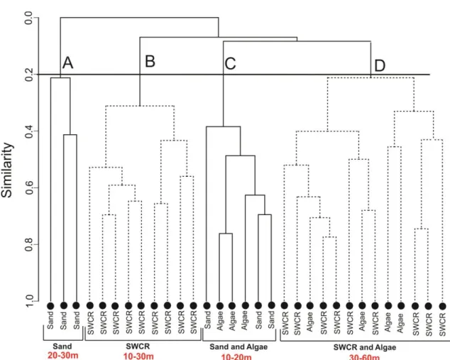
The cluster analyses based on the log-transformed dataset exhibited four major 6
groups (assemblages) at the resemblance level of 20% (Figure 3), showing a significant 7
difference in the species composition among habitats types (R=0.192, p=0.042) and depth 8
range (R=0.201, p=0.001). Assemblage A (named Sand 20-30 m) included only the 9
habitat Sand located on the depth range of 20-30 m. Assemblage B (named SWCR 10-30 10
m) was comprised entirely of SWCR habitat (Sand with coralline formations and 11
sponges), distributed in areas between 10-30 m depth. Assemblage C (named Sand and 12
Algae 10-20 m), with 4 stations, was divided equally between Sand and Algae habitat, 13
both located in shallow areas (10-20 m). Assemblage D (named SWCR and Algae 30-60 14
m), grouped most part of the stations (13), encompassed the SWCR (9 stations) and Algae 15
(4 stations) habitats. All stations for this group were located on depths between 30 and 60 16
m. 17
SIMPER analysis showed low-moderate average within-group similarity ranging 18
from 29.2 to 55.7% (Table 3). There were only three consolidating species (those 19
cumulatively contributing to over 70% to the similarity) in Assemblage A: 20
Acanthostracion quadricornis, Lactophrys trigonus and Hypanus marianae. Assemblage
21
B had the greatest number of consolidating species (13), with Lutjanus synagris, 22
Eucinostomus argenteus and Bothus ocellatus contributing to the highest percentage
23
(29.2%). In Assemblage C, with 7 consolidating species, Acanthostracion polygonius, 24
Eucinostomus gula and Lutjanus synagris cumulatively contributed to the highest
25
contribution (36.6%). Assemblage D was composed by 9 consolidating species, with 26
Acanthostracion polygonius, Diodon holocanthus, Acanthostracion quadricornis and
27
Hypanus marianae showing the highest contribution (48 %).
28
The dissimilarity levels between the assemblages were much higher than the 29
within-assemblage similarity, ranging from 71.9% (B-C) to 81.9% (D-A) (Table 4). 30
Discriminating species (those cumulatively contributing to over 70% of the dissimilarity) 31
were more numerous than the consolidating species within assemblages, ranging from 18 32
to 29 species. Dissimilarities between assemblages B-A, D-A and A-C were primarily a 33
result of species that were absent (e.g. Eucinostomus argenteus, Eucinostomus Gula, 34
Lutjanus synagris and Diodon holocanthus) from one or other of the assemblages.
35
However, between D-B, B-C and D-C the dissimilarity was driven mostly by differences 36
in average abundance rather than presence/absence. 37
39
40
Figure 3 – Dendrogram showing habitat types and depth range obtained after cluster analysis applied on
41
the Bray Curtis similarities calculated among hauls (abundance data) for demersal fish assemblage in the
42
northeast Brazilian continental shelf (4°-9°S). SWCR is the habitat sand with coralline formations and
43
sponges.
44 45
Table 3 -SIMPER results of demersal fish species contributing > 70 % of similarity for the four community
46
assemblages (A, B, C and D) at the northeast Brazilian continental shelf identified using cluster analysis
47
(4°-9°S). Av. abund. is the average abundance, Av. Sim is the average similarity, Sim/SD is the ration
48
between similarity and standard deviation, Contrib% is the percentage of similarity contribution and Cum%
49
is the cumulative percentage of the total similarity.
50 51
52 53
Table 4 - Global dissimilarity calculated through SIMPER analyses between the four community
54
assemblages (A, B, C and D) at the northeast Brazilian continental shelf identified using cluster analysis
55
(4°-9°S).
56
Assemblages Global average dissimilarity B-C 71.89 D-A 81.91 D-B 70.58 A-C 77.2 B-A 72.68 D-C 74.71 57 58 59 60 61 62
Species Av. Abund Av. Sim Sim/SD Contrib% Cum. %
Assemblage A - Sand 20-30m: average similarity = 29.2
Acanthostracion quadricornis 21.57 14.66 3.35 48.91 48.91
Lactophrys trigonus 14.64 4.9 0.58 16.36 65.27
Hypanus marianae 14.87 3.53 0.58 11.78 77.05
Assemblage B - SWCR 10- 30m: average similarity = 47.55
Lutjanus synagris 21.25 5.25 6.42 11.05 11.05
Eucinostomus argenteus 19.59 4.36 1.75 9.17 20.22
Bothus ocellatus 19.28 4.29 1.76 9.01 29.23
Synodus foetens 16.99 3.34 1.14 7.03 36.26
Assemblage C- Sand and Algae 10-20: average similarity = 55.69
Acanthostracion polygonius 22.29 6.96 5.39 12.5 12.5
Eucinostomus gula 21.66 6.75 5.33 12.12 24.62
Lutjanus synagris 21.6 6.72 5.22 12.07 36.69
Haemulon steindachneri 21.31 6.64 5.02 11.93 48.62
Assemblage D- SWCR and Algae 30-60: average similarity = 46.76
Acanthostracion polygonius 19.99 5.38 2.02 11.51 11.51
Diodon holocanthus 20.09 5.22 2.02 11.16 22.67
Acanthostracion quadricornis 18.28 4.4 1.39 9.42 32.1
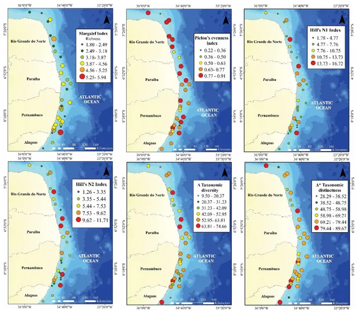
Margalef richness index d ranged from 0.48 to 5.93, with higher values in the south of 63
Pernambuco (PE) (8°S - 9°S) (p<0.05). Stations with comparatively low values of richness 64
were observed along the entire study area. However, the state of Rio Grande do Norte 65
aggregated most part of them (5° - 6°S) (Figure 4). Hill’s N1 and N2 indices varied between 66
1.65 to 16.72 effective species and 1.27 and 11.71 effective species, respectively. Based on 67
Hill’s indices, elevated values of diversity were found in specific locations along the entire 68
latitudinal range, with almost all higher values located in the deepest locations (40-60m) 69
(Figure 4). Pielou’s evenness indicated a high equitability (0.77 -0.91) along the whole study 70
area, ranging from 0.23 to 0.95 and showing no significant differences among latitudes and 71
depth (Figure 4). The taxonomic diversity (Δ) and Taxonomic distinctness (Δ*) indices varied 72
from 9.5 to 74.7 and 28.3 to 89.7, respectively. Most part of higher values of taxonomic indices 73
found in the state of PE and Paraiba (PB) were sampled near to the shore (Figure 3). 74
In relation to assemblages, higher values of richness and taxonomic diversity were 75
found for assemblage B (p<0.05), followed, in the decreasing order, by the assemblages C, D, 76
and A (Figure 4). Hill’s N1 and N2 indices presented higher values of diversity for assemblage 77
C, followed by assemblages D, B and A (p<0.05) (Figure 5). The taxonomic distinctness and 78
Pielou’s evenness indices did not show significant differences among assemblages (p>0.05). 79
80
81
Figure 4 - Spatial representation of estimations of Margalef index, Pielou’s evenness, Hill’s Shannon index (N1),
82
Hill’s Simpson’s index (N2) and taxonomic diversity (Δ) and Taxonomic distinctness (Δ*) of demersal fishes
83
caught along the northeast Brazilian continental shelf (4°- 9°S).
84 85 86
87
Figure 5 – Box plot of Margalef index, Pielou’s evenness, Hill’s Shannon index (N1), Hill’s Simpson’s index
88
(N2) and taxonomic diversity (Δ) and Taxonomic distinctness (Δ*) per assemblages from cluster analysis on
89
demersal fishes caught along the northeast Brazilian continental shelf (4°- 9°S).
90 91
4. DISCUSSION
92
The fish diversity found in the Brazilian northeast continental shelf (120 demersal fish 93
species) is, overall, similar or higher than other tropical coastal shelf ecosystems in Brazil 94
(MMA, 2006), and around the world. For instance, in tropical systems, Willems and Backer 95
(2015) reported 98 species in Suriname and Gray and Otway (1994) observed 75 species in 96
Australia. In temperate areas, Beentjes et al. (2002) registered 100 species in New Zealand, 97
Jaureguizar et al. (2006) reported 94 species in Argentine and Prista et al. (2003) observed 36 98
species in Portugal. On the opposite, higher demersal fish diversity has been reported in Costa 99
Rica and Southern Tyrrhenian Sea, with 242 and 249 species, respectively (Busalacchi et al., 100
2010; Sousa et al., 2006; Wolff, 1996). Besides intrinsic biogeographic differences (e.g. 101
oceanographic conditions, climate pattern, habitat heterogeneity) (Ray and Grassle, 1991), 102
which are major factors driving the number of species, sampling strategy and effort were 103
different among studies, which may also affect the observed image of the diversity (Magurran, 104
2004). 105
The dominance pattern found in demersal fish assemblages of the Brazilian northeast 106
continental shelf is probably related to habitat type, once most of the dominant families are 107
classified as distinctive reef-associated (e.g. Haemulidae, Lutjanidae) (Rangel et al., 2007). In 108
addition, some of the dominant species also share the same food resource (sessile and mobile 109
invertebrates) (Bowen et al., 1995; Rangel et al., 2007). The dominance of the demersal 110
assemblage by few families (7 out of 49) has also been registered in other studies in Brazil 111
(Azevedo et al., 2007; Muto et al., 2000) and elsewhere (Jaureguizar et al., 2006; Johannesen 112
et al., 2012; Prista et al., 2003), seeming to be an ecological pattern of demersal assemblages 113
(Gibson et al., 2007). 114
The highest values of richness (expressed through Margalef index) were found in the 115
south of Pernambuco (8°30’S - 9°). This area encompassed species classified as highly 116
abundant and frequent but also most of the species classified as lower abundant and rare, 117
including species currently categorized as Vulnerable by IUCN (e.g. Sparisoma axillare, S. 118
frondosum and M. bonaci). Many species are also categorized as Data Deficient (DD). A wide
119
range of variables drives the number of species of a location (e.g. human activity, physical 120
factors, prey availability) (Ray and Grassle, 1991). The presence and extension of coral reefs 121
and associated ecosystems found in the south of Pernambuco (Costa et al., 2007; Ferreira et 122
al., 2006) as well as their conservation status, have motivated the creation of two Marine 123
Protected Areas (‘APA Costa do Corais’ and ‘APA Guadalupe’) (Ferreira and Maida, 2007; 124
Prates et al., 2007), that are now probably the main factor responsible for the maintenance of 125
such richness. The ‘APA Costa do Corais’ (ACC) was created in 1997, encompassing more 126
than 400 thousand hectares of marine area. Although artisanal fisheries are allowed inside the 127
ACC, and law enforcement is a challenge in these large areas, increased compliance may be a 128
possible expected effect (Gerhardinger et al., 2011; Pollnac et al., 2010). Zoning, for instance, 129
includes the creation of no-taken zones, where a rapid increase of richness, diversity, and 130
biomass of many species have been observed (Ferreira and Maida, 2007). 131
High values of diversity (Pielou and Hill’s indices) were found in specific locations 132
along the entire latitudinal range, with almost all higher values located in the deepest habitats 133
(30 -60m). Previous studies based on underwater visual sensing and bottom long-lines have 134
also reported high values of diversity in deep coastal shelf environments on the Brazilian coast 135
(Feitoza et al., 2005; Olavo et al., 2011). This location is indeed a marine ecotone characterized 136
by the coexistence of different communities of the continental shelf, upper slope and adjacent 137
pelagic biota (Olavo et al., 2011). This ecotone, characterized by high population densities and 138
species richness, concentrates fishing resources and sustain an important multispecific reef 139
fishery in the Tropical Atlantic (Costa et al., 2005; Frédou and Ferreira, 2005; Olavo et al., 140
2011). In addition, these deep coastal shelf environments on the Brazilian coast are part of a 141
faunal corridor that serves as a connection between cold habitats in southern Brazil and the 142
Caribbean (Olavo et al., 2011). Finally, the occurrence of small upwelling processes has been 143
reported near to these locations enhancing nutrient supply from deeper layers and increasing 144
food availability for fish assemblages (MMA, 2006). 145
Taxonomic diversity (∆) and distinctness (∆*), which consider taxonomic differences 146
between species, presented high values distributed along the whole study area, evidencing the 147
presence of local hotspots supporting higher diversity. Most high values of taxonomic indices 148
were found in the shallowest habitats (10-30m). This result shows that, although the deepest 149
habitats (30-60m) holds the highest values of diversity (N1 and N2), the shallowest habitats 150
contains species that are more taxonomically distant. This pattern was largely driven by the 151
presence of rays (Dasyatis spp.), which were more abundant in sand shallow habitats near to 152
the coast. Indeed, habitat and bathymetric segregation are known for these species (Costa et 153
al., 2017). This pattern was also reported by Rogers et al. (1999) in the Northeast Atlantic. 154
The major factors structuring assemblages were habitat type and depth strata. Despite 155
the distinctive influence of habitat, the assemblages C and D were related to more than one 156
habitat type. It may be explained by the great mobility and feeding behavior of many species 157
found in this study (e.g. L. synagris, P. maculatus and H. plumierii) that may move between 158
habitats according to their use for food and shelter (Mora, 2015). In addition, the similarity 159
percentage procedure (SIMPER) revealed that many species are usually present in more than 160
one habitat type. Assemblages C (composed by Sand and Algae) and D (composed by SWCR 161
and Algae) presented the highest values of diversity (N1 and N2). This pattern is not only a 162
consequence of the presence of more complex habitats, which increases diversity, but also a 163
consequence of the ecological benefits provided by these locations. Habitats as algae and 164
coralline formations mediate competition and predation, facilitate cohabitation of an increased 165
number of species, and provide essential habitats and resources for marine invertebrates and 166
fish (Bertelli and Unsworth, 2014; Darling et al., 2017). The highest values richness and 167
taxonomic diversity were found in the assemblages B, which comprise only SWCR habitats in 168
relatively shallow waters (10-30 m depth). 169
5. CONCLUSION
170
Our results may be hampered by gear selectivity and by the sampling spatial extent. We 171
do not propose an exhaustive inventory of demersal fish assemblages in the northeast Brazilian 172
coast, but our results provide valuable information on tropical fish fauna distribution in this 173
area, and relationships with habitat characteristics. These findings are useful for conservation 174
purposes. Indeed, we identified the presence of numerous sensitive and commercial species 175
deserving special attention from stakeholders since they are currently categorized within risk 176
categories by IUCN or Data Deficient. These species are mainly associated with the habitat 177
SWCR, which also holds the highest number of species classified as scarce/rare and the greatest 178
values of biodiversity. We also highlight the importance of the deepest coastal shelf 179
environments (30-60 m) as areas of high fish densities and diversity. 180
Ecosystem-based management practices have been implemented with the creation of 181
marine protected areas encompassing interconnected habitats in a portion of the study area 182
(Ferreira and Maida, 2007; Prates et al., 2007). However, most critical environments identified 183
in this study remain unprotected. We thus recommend giving special attention on SWCR 184
habitats, mainly those located close to the shelf-break, between 30 and 60 m of depth, in 185
management strategies of conservation. Possible measures include specific regulations of use 186
and/or creation or expansion of MPAs encompassing those environments (CBD, 2014). 187
Acknowledgements
188
We acknowledge the French oceanographic fleet for funding the at-sea survey Abraços 1 and 2
189
(http://dx.doi.org/10.17600/15005600 / http://dx.doi.org/10.17600/17004100) and the officers and crew of the R/V
190
Antea for their contribution to the success of the operations. The present study could not have been done without
191
the work of all participants from the BIOIMPACT Laboratory. We thank the CNPq (Brazilian National Council for
192
Scientific and Technological Development), which provided student scholarship to Leandro Nolé Eduardo and Alex
193
Souza Lira and research grant for Thierry Frédou, Beatrice Padovani Ferreira and Flávia Lucena Frédou. This work
194
is a contribution to the LMI TAPIOCA and the EU RISE Project PADDLE.
195
Funding: This study was funded by the French oceanographic fleet, through the projects ABRACOS 1 and 2 196
(http://dx.doi.org/10.17600/15005600 / http://dx.doi.org/10.17600/17004100).
197
Ethical approval: All applicable international, national, and/or institutional guidelines for the care and use of 198
animals were followed. All procedures performed in this research were in accordance with the ethical standards of
199
the the institution (University Federal Rural de Pernambuco) and the Brazilian Ministry of Envirnomental.
6. REFERENCES
201
Anderson, M.J., Gorley, R.N., Clarke, K.R., 2008. PERMANOVA+ for PRIMER: Guide to 202
Software and Statistical Methods. PRIMER-E, Plymouth. 203
Azevedo, M.C.C. d, Araújo, F.G., Cruz-Filho, A.G. d, Pessanha, A.L.M., Silva, M. d A., 204
Guedes, A.P.P., 2007. Demersal fishes in a tropical bay in southeastern Brazil: 205
Partitioning the spatial, temporal and environmental components of ecological variation. 206
Estuar. Coast. Shelf Sci. 75, 468–480. doi:10.1016/j.ecss.2007.05.027 207
Beentjes, M.P., Bull, B., Hurst, R.J., Bagley, N.W., 2002. Demersal fish assemblages along the 208
continental shelf and upper slope of the east coast of the South Island, New Zealand. New 209
Zeal. J. Mar. Freshw. Res. 36, 197–223. doi:10.1080/00288330.2002.9517080 210
Bertelli, C.M., Unsworth, R.K.F., 2014. Protecting the hand that feeds us: Seagrass (Zostera 211
marina) serves as commercial juvenile fish habitat. Mar. Pollut. Bull. 83, 425–429. 212
doi:10.1016/j.marpolbul.2013.08.011 213
Borcard, D., Gillet, F., Legendre, P., 2011. Numerical Ecology with R, 1st ed, Media. Springer 214
New York Dordrecht London Heidelberg, Québec. 215
Bowen, S.H., Lutz, E. V., Ahlgren, M.O., 1995. Bowen SH, Lutz E V., Ahlgren MO (1995) 216
Dietary protein and energy as determinants of food quality: Trophic strategies compared. 217
Ecology 76:899–907. doi: 10.2307/1939355Dietary protein and energy as determinants 218
of food quality: Trophic strategies compared. Ecology 76, 899–907. doi:10.2307/1939355 219
Busalacchi, B., Rinelli, P., De Domenico, F., Profeta, A., Perdichizzi, F., Bottari, T., 2010. 220
Analysis of demersal fish assemblages off the Southern Tyrrhenian Sea (central 221
Mediterranean). Hydrobiologia 654, 111–124. doi:10.1007/s10750-010-0374-9 222
Causse, R., Ozouf-Costaz, C., Koubbi, P., Lamy, D., Eléaume, M., Dettaï, A., Duhamel, G., 223
Busson, F., Pruvost, P., Post, A., Beaman, R.J., Riddle, M.J., 2011. Demersal 224
ichthyofaunal shelf communities from the Dumont d’Urville Sea (East Antarctica). Polar 225
Sci. 5, 272–285. doi:10.1016/j.polar.2011.03.004 226
CBD, 2014. Ecologically or Biologically Significant Marine Areas (EBSAs). Special places in 227
the world’s oceans., 2nd ed. Secretariat of the Convention on Biological Diversity, Recife. 228
Clarke, K., Somerfield, P.J., Warwick, R., 1994. Change in marine communities: an approach 229
to statistical analysis and interpretation, 1st ed. PRIMER-E Ltd, Plymouth. 230
Costa, P., Martins, A., Olavo, G., Haimovici, M., Braga, A., 2005. Pesca exploratória com 231
arrasto de fundo no talude continental da região central da costa brasileira entre Salvador-232
BA e o cabo de São Tomé-RJ, in: Pescae Potenciais de Exploração de Recursos Vivos Na 233
Região Central Da Zona Econômica Exclusiva Brasileira. Museu Nacional, Rio de 234
Janeiro, pp. 145–165. 235
Costa, P., Olavo, G., Martins, A.S., 2007. Biodiversidade na costa central brasileira. Museu 236
Nacional, Rio de Janeiro. 237
Costa, T.L.A., Pennino, M.G., Mendes, L.F., 2017. Identifying ecological barriers in marine 238
environment: The case study of Dasyatis marianae. Mar. Environ. Res. 125, 1–9. 239
doi:10.1016/j.marenvres.2016.12.005 240
Curley, B.G., Kingsford, M.J., Gillanders, B.M., 2002. Spatial and habitat-related patterns of 241
temperate reef fish assemblages: Implications for the design of Marine Protected Areas. 242
Mar. Freshw. Res. 53, 1197–1210. doi:10.1071/MF01199 243
Dahl, R., Ehler, C., Douvere, F., 2009. Marine spatial planning: A Step-by-Step Approach 244
toward ecosystem based management, UNESCO IOC Manual and Guides. 245
Intergovernmental Oceanographic Commission and Man and the Biosphere Programme, 246
Paris. 247
Darling, E.S., Graham, N.A.J., Januchowski-hartley, F.A., Nash, K.L., Pratchett, M.S., Wilson, 248
S.K., 2017. Relationships between structural complexity , coral traits , and reef fish 249
assemblages. Coral Reefs 36, 561–575. doi:10.1007/s00338-017-1539-z 250
Ekau, W., Knoppers, B., 1999. An introduction to the pelagic system of the north-east and east 251
Brazilian shelf. Arch. Fish. Mar. Res. 47, 113–132. doi:0944-1921/99/47/2/3-5/12.00$/0 252
Farriols, M.T., Ordines, F., Somerfield, P.J., Pasqual, C., Hidalgo, M., Guijarro, B., Massutí, 253
E., 2017. Bottom trawl impacts on Mediterranean demersal fish diversity: Not so obvious 254
or are we too late? Cont. Shelf Res. 137, 84–102. doi:10.1016/j.csr.2016.11.011 255
Feitoza, B.M., Rosa, R.S., Rocha, L.A., 2005. Ecology and Zoogeography of Deep- Reef 256
Fishes in Northeastern Brazil. Bull. Mar. Sci. 76, 725–742. 257
Ferreira, B.P.., Toniolo, L.M.., Maida, M., 2006. The Environmental Municipal Councils as an 258
Instrument in Coastal Integrated Management: the Área de Proteção Ambiental Costa dos 259
Corais (AL/ PE) Experience. J. Coast. Res. 39, 1003–1007. 260
Ferreira, B.P., Maida, M., 2007. Características e Perspectivas para o Manejo da Pesca na Área 261
de Proteção Ambiental Marinha da Costa dos Corais, in: Áreas Aquáticas Protegidas 262
Como Instrumento de Gestão Pesqueira. Serie Areas Protegidas, Brasília, pp. 39–51. 263
Ferreira, C.E.L., Floeter, S.R., Gasparini, J.L., Ferreira, B.P., Joyeux, J.C., 2004. Trophic 264
structure patterns of Brazilian reef fishes: A latitudinal comparison. J. Biogeogr. 31, 265
1093–1106. doi:10.1111/j.1365-2699.2004.01044.x 266
Frédou, T., Ferreira, B.P., 2005. Bathymetric trends of northeastern Brazilian snappers (pisces, 267
lutjanidae): Implications for the reef fishery dynamic. Brazilian Arch. Biol. Technol. 48, 268
787–800. doi:10.1590/S1516-89132005000600015 269
Gaertner, J.-C., Bertrand, J., Gil de Sola, L., Durbec, J.-P., Ferrandis, E., Souplet, A., 2005. 270
Large spatial scale variation of demersal fish assemblage structure on the continental shelf 271
of the NW Mediterranean Sea. Mar. Ecol. Prog. Ser. 297, 245–257. 272
doi:10.3354/meps297245 273
Garcia, A.M., Bemvenuti, M.A., Vieira, J.P., Motta Marques, D.M.L., Burns, M.D.M., 274
Moresco, A., Vinicius, M., Condini, L., 2006. Checklist comparison and dominance 275
patterns of the fish fauna at Taim Wetland, South Brazil. Neotrop. Ichthyol 4, 261–268. 276
Gerhardinger, L.C., Godoy, E.A.S., Jones, P.J.S., Sales, G., Ferreira, B.P., 2011. Marine 277
protected dramas: The flaws of the Brazilian national system of marine protected areas. 278
Environ. Manage. 47, 630–643. doi:10.1007/s00267-010-9554-7 279
Gibson, R.N., Atkinson, R.J. a, Gordon, J.D.M., 2007. Oceanography and Marine Biology An 280
Annual Review Vol.45. Taylor & Francis, Boca Raton, FL. 281
Gray, C.A., Otway, N.M., 1994. Spatial and temporal differences in assemblages of demersal 282
fishes on the inner continental shelf off sydney, south-eastern australia. Mar. Freshw. Res. 283
45, 665–676. doi:10.1071/MF9940665 284
Gregory, S., Collins, M.A., Belchier, M., 2016. Demersal fish communities of the shelf and 285
slope of South Georgia and Shag Rocks (Southern Ocean). Polar Biol. 40, 107–121. 286
doi:10.1007/s00300-016-1929-7 287
Halpern, B.S., 2003. The impact of marine reserves: do reserves work and does reserve size 288
matter? Ecol. Appl. 13, 117–137.
doi:10.1890/1051-289
0761(2003)013[0117:TIOMRD]2.0.CO;2 290
Hanchet, S.M., Stewart, A.L., McMillan, P.J., Clark, M.R., O’Driscoll, R.L., Stevenson, M.L., 291
2013. Diversity, relative abundance, new locality records, and updated fish fauna of the 292
Ross Sea region. Antarct. Sci. 25, 619–636. doi:10.1017/S0954102012001265 293
Hill, M.O., 1973. Diversity and evenness: a unifying notation and its consequences. Ecology 294
54, 427–432. doi:10.2307/1934352 295
ICMbio, 2016. Executive Summary Brazil Red Book of Threatened Species of Fauna sumario, 296
Livro Vermelho. Instituto Chico Mendes de Conservaçã o da Biodiversidade, Ministério 297
de Meio Ambiente, Brasília, DF. 298
IUCN, 2012. Guidelines for Application of IUCN Red List Criteria at Regional and National 299
Levels: Version 4.0. IUCN, Gland, Switzerland and Cambridge, UK. 300
IUCN, 2000. IUCN Red List Categories and Criteria, IUCN Bulletin. IUCN, Gland, 301
Switzerland and Cambridge, UK. doi:10.9782-8317-0633-5 302
Jaureguizar, A.J., Menni, R., Lasta, C., Guerrero, R., 2006. Fish assemblages of the northern 303
Argentine coastal system: Spatial patterns and their temporal variations. Fish. Oceanogr. 304
15, 326–344. doi:10.1111/j.1365-2419.2006.00405.x 305
Johannesen, E., Hoines, A.S., Dolgov, A. V., Fossheim, M., 2012. Demersal fish assemblages 306
and spatial diversity patterns in the arctic-atlantic transition zone in the barents sea. PLoS 307
One 7. doi:10.1371/journal.pone.0034924 308
Laliberté, E., Legendre, P., 2010. A distance-based framework for measuring functional 309
diversity from multiple traits. Ecology 91, 299–305. 310
Letessier, T.B., Meeuwig, J.J., Gollock, M., Groves, L., Bouchet, P.J., Chapuis, L., Vianna, 311
G.M.S., Kemp, K., Koldewey, H.J., 2013. Assessing pelagic fish populations: The 312
application of demersal video techniques to the mid-water environment. Methods 313
Oceanogr. doi:10.1016/j.mio.2013.11.003 314
Lotze, H.K., Lenihan, H.S., Bourque, B.J., Bradbury, R.H., Cooke, R.G., Kay, M.C., Kidwell, 315
S.M., Kirby, M.X., Peterson, C.H., Jackson, J.B.C., 2006. Depletion, Degradation, and 316
Recovery Potential of Estuaries and Coastal Seas. Science (80-. ). 312, 1806–1809. 317
doi:10.1126/science.1128035 318
Magurran, A.E., 2004. Measuring biological diversity. Blackwell Pub, Malden. 319
Margalef, R.D., 1978. Information Theory In Ecology. Gen. Syst. 320
Mellin, C., Andréfouët, S., Kulbicki, M., Dalleau, M., Vigliola, L., 2009. Remote sensing and 321
fish-habitat relationships in coral reef ecosystems: Review and pathways for multi-scale 322
hierarchical research. Mar. Pollut. Bull. 58, 11–19. doi:10.1016/j.marpolbul.2008.10.010 323
Miloslavich, P., Klein, E., Díaz, J.M., Hernández, C.E., Bigatti, G., Campos, L., Artigas, F., 324
Castillo, J., Penchaszadeh, P.E., Neill, P.E., Carranza, A., Retana, M. V, Díaz de Astarloa, 325
J.M., Lewis, M., Yorio, P., Piriz, M.L., Rodríguez, D., Valentin, Y.Y., Gamboa, L., 326
Martín, A., 2011. Marine biodiversity in the Atlantic and Pacific coasts of South America: 327
Knowledge and gaps. PLoS One 6. doi:10.1371/journal.pone.0014631 328
MMA, 2006. Programa REVIZEE. Avaliação do Potencial Sustentável de Recursos Vivos na 329
Zona Econômica Exclusiva. Ministério do Meio Ambiente, Brasília, DF. 330
Muto, E.Y., Soares, L.S.H., Rossi-wongtschowski, C.L.D.B., 2000. Demersal fish assemblages 331
off São Sebastião, southeatern Brazil: structure and environmental conditioning factors 332
(summer 1994). Rev. Bras. Oceanogr. 48, 9–27. doi:10.1590/S1413-77392000000100002 333
Nelson, J.S., Grande, T., Wilson, M.V.H., 2016. Fishes of the world, 5th ed. Wiley. 334
Nóbrega, M.F. de, Lessa, R., Santana, F.M., 2009. Peixes Marinhos da regiao Nordeste do 335
Brasil. Martins & Cordeiro, Fortaleza. 336
Oksanen, J., F. Guillaume Blanchet, M.F., Kindt, R., Legendre, P., Dan McGlinn, P.R.M., 337
Simpson, L., Solymos, P., Henry, M., Stevens, H., 2017. Vegan: Community Ecology 338
Package. 339
Olavo, G., Costa, P.A.S., Martins, A.S., Ferreira, B.P., 2011. Shelf-edge reefs as priority areas 340
for conservation of reef fish diversity in the tropical Atlantic. Aquat. Conserv. Mar. 341
Freshw. Ecosyst. 21, 199–209. doi:10.1002/aqc.1174 342
Pielou, E.C., 1966. Species-diversity and pattern-diversity in the study of ecological 343
succession. J. Theor. Biol. 10, 370–383. doi:http://dx.doi.org/10.1016/0022-344
5193(66)90133-0 345
Pollnac, R., Christie, P., Cinner, J.E., Dalton, T., Daw, T.M., Forrester, G.E., Graham, N.A.J., 346
McClanahan, T.R., 2010. Marine reserves as linked social-ecological systems. Proc. Natl. 347
Acad. Sci. 107, 18262–18265. doi:10.1073/pnas.0908266107 348
Prates, A.P.L., Cordeiro, A.Z., Ferreira, B.P., Maida, M., 2007. Unidades de Conservação 349
Costeiras e Marinhas de Uso Sustentável como Instrumento para a Gestão Pesqueira, in: 350
Áreas Aquáticas Protegidas Como Instrumento de Gestão Pesqueira. Serie Areas 351
Protegidas, Brasília, pp. 27–39. 352
Prista, N., Vasconcelos, R.P., Costa, M.J., Cabral, H., 2003. The demersal fish assemblage of 353
the coastal area adjacent to the Tagus estuary (Portugal): Relationships with 354
environmental conditions. Oceanol. Acta 26, 525–536. doi:10.1016/S0399-355
1784(03)00047-1 356
R Core Team, 2016. R: A language and environment for statistical computing. R Foundation 357
for Statistical Computing, Vienna, Austria. 358
Rangel, C.A., Chaves, L.C.T., Monteiro-Neto, C., 2007. Baseline Assessment of the Reef Fish 359
Assemblage From Cagarras Archipelago, Rio De Janeiro, Southeastern Brazil. Brazilian 360
J. Oceanogr. 55, 7–17. doi:10.1590/S1679-87592007000100002 361
Ray, G.C., Grassle, J.F., 1991. Marine Biological Diversity Program. Bioscience 41, 453–457. 362
doi:10.2307/1311799 363
Roberts, C.M., Bohnsack, J.A., Gell, F., Hawkins, J.P., Goodridge, R., 2001. Effects of marine 364
reserves on adjacent fisheries. Science 294, 1920–3. doi:10.1126/science.294.5548.1920 365
Rogers, S.I., Clarke, K.R., Reynolds, J.D., 1999. The Taxonomic Distinctness of Coastal 366
Botton-Dwelling Fish Communities of the North-East Atlantic. J. Anim. Ecol. 68, 769– 367
782. doi:10.1046/j.1365-2656.1999.00327.x 368
Silva Júnior, C.A.B. da, Viana, A.P., Frédou, F.L., Frédou, T., 2015. Aspects of the 369
reproductive biology and characterization of Sciaenidae captured as bycatch in the prawn 370
trawling in the northeastern Brazil. Acta Sci. Biol. Sci. 37, 1. 371
doi:10.4025/actascibiolsci.v37i1.24962 372
Sousa, P., Azevedo, M., Gomes, M.C., 2006. Species-richness patterns in space, depth, and 373
time (1989-1999) of the Portuguese fauna sampled by bottom trawl. Aquat. Living 374
Resour. 19, 93–103. doi:10.1051/alr:2006009 375
Vital, H., Gomes, M.P., Tabosa, W.F., Fraz??o, E.P., Santos, C.L.A., Placido Junior, J.S., 2010. 376
Characterization of the Brazilian continental shelf adjacent to Rio Grande do Norte State, 377
Ne Brazil. Brazilian J. Oceanogr. 58, 43–54. doi:10.1590/S1679-87592010000500005 378
Warwick, R.M., Clarke, K.R., 1995. New “biodiversity’’ measures reveal a decrease in 379
taxonomic distinctness with increasing stress.” Mar. Ecol. Prog. Ser. 129, 301–305. 380
doi:10.3354/meps129301 381
Willems Tomas; Backer, A.M.J.H.. V.M.H.K., 2015. Distribution patterns of the demersal fish 382
fauna on the inner continental shelf of Suriname. Reg. Stud. Mar. Sci. 2, 177–188. 383
doi:10.1016/j.rsma.2015.10.008 384
Wolff, M., 1996. Demersal fish assemblages along the Pacific coast of Costa Rica: a 385
quantitative and multivariate assessment hased on the Victor Hensen Costa Rica 386
Expedition (199311994). Rev. Biol. Trop. 44, 187–214. 387
Worm, B., Barbier, E.B., Beaumont, N., Duffy, J.E., Folke, C., Halpern, B.S., Jackson, J.B.C., 388
Lotze, H.K., Micheli, F., Palumbi, S.R., Sala, E., Selkoe, K.A., Stachowicz, J.J., Watson, 389
R., 2006. Impacts of Biodiversity Loss on Ocean Ecosystem Services. Science (80-. ). 390 314, 787–790. doi:10.1126/science.1132294 391 392 393 394 395 396 397 398 399 400 401 402 403
Supplementary Material 1- Size histogram of fish captured during the Abraços 1 (red) and 2 (blue) surveys
404
in the latitudinal range 4°- 9°S.
405 406
407
408
Supplementary Material 2- Spatial representation of bottom environmental variables collected using a
409
CTD along the northeast Brazilian continental shelf (4°- 9°S).
410 411 412 413 414 415 416 417 418 419 420 421 422 423 424 425 426
Supplementary Material 3- CTD profiles of environmental variables collected through two surveys along
427
the northeast Brazilian continental shelf (4°- 9°S).
428 429 430 431
432
Supplementary material 4 -SIMPER results of demersal fish species contributing > 70 % of similarity for the four
433
community assemblages (A, B, C and D) at the northeast Brazilian continental shelf identified using cluster
434
analysis (4°-9°S).
435
Species Av. Abund Av. Sim Sim/SD Contrib% Cum. %
Assemblage A - Sand 20-30m: average similarity = 29.2
Acanthostracion quadricornis 21.57 14.66 3.35 48.91 48.91
Lactophrys trigonus 14.64 4.9 0.58 16.36 65.27
Hypanus marianae 14.87 3.53 0.58 11.78 77.05
Assemblage B - SWCR 10- 30m: average similarity = 47.55
Lutjanus synagris 21.25 5.25 6.42 11.05 11.05 Eucinostomus argenteus 19.59 4.36 1.75 9.17 20.22 Bothus ocellatus 19.28 4.29 1.76 9.01 29.23 Synodus foetens 16.99 3.34 1.14 7.03 36.26 Hypanus marianae 14.79 2.17 0.82 4.56 40.83 Stephanolepis hispidus 14.69 1.99 0.83 4.19 45.01 Haemulon plumierii 14.7 1.99 0.83 4.18 49.19 Syacium micrurum 14.72 1.98 0.83 4.16 53.35 Pseudupeneus maculatus 14.45 1.96 0.82 4.12 57.47 Diodon holocanthus 14.41 1.94 0.83 4.08 61.55 Trachinocephalus myops 11.95 1.4 0.6 2.94 64.48 Synodus intermedius 12.01 1.37 0.6 2.89 67.37 Holocentrus adscensionis 12.1 1.34 0.61 2.81 70.18
Assemblage C- Sand and Algae 10-20: average similarity = 55.69
Acanthostracion polygonius 22.29 6.96 5.39 12.5 12.5 Eucinostomus gula 21.66 6.75 5.33 12.12 24.62 Lutjanus synagris 21.6 6.72 5.22 12.07 36.69 Haemulon steindachneri 21.31 6.64 5.02 11.93 48.62 Pseudupeneus maculatus 21.11 6.49 4.99 11.66 60.28 Hypanus marianae 18.29 4.03 1.34 7.25 67.53 Diplectrum formosum 15.03 2.52 0.78 4.53 72.06
Assemblage D- SWCR and Algae 30-60: average similarity = 46.76
Acanthostracion polygonius 19.99 5.38 2.02 11.51 11.51 Diodon holocanthus 20.09 5.22 2.02 11.16 22.67 Acanthostracion quadricornis 18.28 4.4 1.39 9.42 32.1 Hypanus marianae 18.17 4.14 1.4 8.87 40.96 Pseudupeneus maculatus 17.28 3.61 1.28 7.73 48.69 Fistularia tabacaria 16.44 3.59 1.04 7.69 56.38 Lactophrys trigonus 14.82 3.03 0.82 6.49 62.87 Holocentrus adscensionis 14.56 2.59 0.84 5.55 68.42 Pomacanthus paru 12.79 1.93 0.67 4.12 72.54 436 437 438