Calibration of muon reconstruction algorithms using an external
muon tracking system at the Sudbury Neutrino Observatory
The MIT Faculty has made this article openly available.
Please share
how this access benefits you. Your story matters.
Citation
Sonley, T.J., R. Abruzzio, Y.D. Chan, C.A. Currat, F.A. Duncan,
J. Farine, R.J. Ford, et al. “Calibration of Muon Reconstruction
Algorithms Using an External Muon Tracking System at the Sudbury
Neutrino Observatory.” Nuclear Instruments and Methods in Physics
Research Section A: Accelerators, Spectrometers, Detectors and
Associated Equipment 648, no. 1 (August 2011): 92–99.
As Published
http://dx.doi.org/10.1016/j.nima.2011.05.054
Publisher
Elsevier
Version
Original manuscript
Citable link
http://hdl.handle.net/1721.1/108677
Calibration of Muon Reconstruction Algorithms Using an External
Muon Tracking System at the Sudbury Neutrino Observatory
T.J. Sonleya,d, R. Abruzzioa, Y.D. Chanb, C.A. Currat1b, F.A. Duncanc,d, J. Farinee, R.J. Fordc,
J.A. Formaggioa,f,∗, N. Gagnonf,d,b,g, A.L. Hallinh,d, J. Heised,g,i, M.A. Howej,f, E. Ilhoffa,
J. Kelseya, J.R. Kleink, C. Kraush,d, A. Kr¨ugere, T. Kutterl, C.C.M. Kyba2k, I.T. Lawsonc,m,
K.T. Leskob, N. McCauley3k, B. Monreal4a, J. Monroea, A.J. Nobled, R.A. Otta, A.W.P. Poonb,
G. Prior5b, K. Rielageg,f, T. Tsuii, B. Wallf, J.F. Wilkersonj,f
aLaboratory for Nuclear Science, Massachusetts Institute of Technology, Cambridge, MA 02139
bInstitute for Nuclear and Particle Astrophysics and Nuclear Science Division, Lawrence Berkeley National Laboratory, Berkeley, CA 94720
cSNOLAB, Sudbury, ON P3Y 1M3, Canada
dDepartment of Physics, Queen’s University, Kingston, Ontario K7L 3N6, Canada eDepartment of Physics and Astronomy, Laurentian University, Sudbury, Ontario P3E 2C6, Canada fCenter for Experimental Nuclear Physics and Astrophysics, and Department of Physics, University of Washington,
Seattle, WA 98195
gLos Alamos National Laboratory, Los Alamos, NM 87545
hDepartment of Physics, University of Alberta, Edmonton, Alberta, T6G 2R3, Canada iDepartment of Physics and Astronomy, University of British Columbia, Vancouver, BC V6T 1Z1, Canada
jDepartment of Physics, University of North Carolina, Chapel Hill, NC
kDepartment of Physics and Astronomy, University of Pennsylvania, Philadelphia, PA 19104-6396 lDepartment of Physics and Astronomy, Louisiana State University, Baton Rouge, LA 70803
mPhysics Department, University of Guelph, Guelph, Ontario N1G 2W1, Canada
Abstract
To help constrain the algorithms used in reconstructing high-energy muon events incident on the Sudbury Neutrino Observatory (SNO), a muon tracking system was installed. The system consisted of four planes of wire chambers, which were triggered by scintillator panels. The system was integrated with SNO’s main data acquisition system and took data for a total of 95 live days. Using cosmic-ray events reconstructed in both the wire chambers and in SNO’s water Cherenkov detector, the external muon tracking system was able to constrain the uncertainty on
the muon direction to better than 0.6◦.
1Current Address: Business Direct, Wells Fargo, San Francisco, CA
2Current address: Institute for Space Sciences, Freie Universit¨at, Berlin, Leibniz-Institute of Freshwater Ecology and Inland Fisheries, Germany
3Current address: Department of Physics, University of Liverpool, Liverpool, UK
4Current address: Department of Physics, University of California Santa Barbara, Santa Barbara, CA 5Current address: CERN (European Laboratory for Particle Physics), Geneva, Switzerland ∗
Corresponding author.
1. Introduction
1
The Sudbury Neutrino Observatory (SNO) was a large water Cherenkov detector optimized
2
for detecting solar neutrinos created from the8B reaction in the main pp fusion chain. In addition
3
to solar neutrinos, the Sudbury Neutrino Observatory was also sensitive to high-energy muons
4
that traverse the volume of the detector. A small fraction of these events are neutrino-induced
5
muons from atmospheric neutrinos, while the large remaining fraction come from cosmic rays
6
created in the upper atmosphere. It is possible to discriminate between these muon sources by
7
looking at the angular distribution of incoming muons. The combination of large depth and the
8
relatively flat topography in the vicinity of the detector attenuates almost all cosmic ray muons
9
entering the detector at zenith angle cos (θz) > 0.4. The study of muon events in the SNO
detec-10
tor provides measurements of the absolute flux of atmospheric neutrinos and constraints on the
11
atmospheric neutrino mixing parameters∆m2
23and θ23[1]. While the latter measurement is more
12
strongly constrained by other experiments [2, 3], the former is unique to the SNO experiment.
13
To facilitate a clean measurement of the zenith distribution of muons entering the SNO
fidu-14
cial volume, an accurate understanding of the muon reconstruction algorithm is necessary. This
15
includes both the angular and spatial resolution of high-energy muons which enter the detector.
16
Determining the accuracy of the muon tracking reconstruction algorithm, however, relies almost
17
entirely on Monte Carlo simulations. Although the detector response to muons was benchmarked
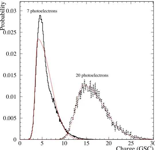
18
against selected cosmic-ray data, there is not an external calibration source that can provide a
19
consistency-check to the accuracy of the reconstruction algorithm. This is in sharp contrast to
20
the case for SNO’s response to neutrons and low energy electrons, which was calibrated with
21
multiple sources to a precision of ∼ 1% [4].
22
We present in this paper a means by which the SNO experiment was able to calibrate its
23
muon tracking algorithm via the use of an external muon tracking system. The External Muon
24
System (EMuS) allowed SNO to simultaneously reconstruct selected cosmic-ray events in two
25
independent systems, thereby providing a cross-check on the tracking algorithm. The EMuS
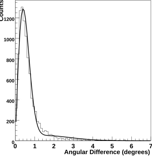
26
experiment ran for a total of 94.6 live days during the last phase of the SNO experiment.
27
This paper is divided as follows: Section 2 describes the main SNO experiment, Section 3
28
describes the SNO muon reconstruction algorithm, Section 4 describes the characteristics of the
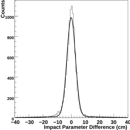
29
EMuS apparatus, Section 5 describes the criterion for accepting events, and finally Section 6
30
discusses the analysis used to calibrate the SNO tracking algorithm against data taken with the
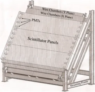
31
EMuS system.
32
2. The Sudbury Neutrino Observatory
33
The SNO detector consisted of a 12-meter-diameter acrylic sphere filled with 1 kiloton of
34
D2O. The 5.5-cm-thick acrylic vessel was surrounded by 7.4 kilotons of ultra-pure H2O encased
35
within a barrel-shaped cavity, 34 m in height and 22 m in diameter. A 17.8-meter-diameter
36
geodesic structure surrounded the acrylic vessel and supported 9456 20-cm-diameter
photomul-37
tiplier tubes (PMTs) pointed toward the center of the detector. A non-imaging light concentrator
38
of 42◦ with respect to the propagation direction of the muon. Cherenkov light and light from
45
delta rays produced by the muon illuminate an average of 5500 PMTs, whose charge and timing
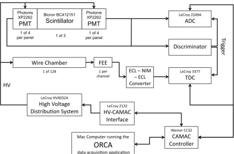
46
information are recorded. The amplitude and timing response of the PMTs were calibrated in
47
situusing a light diffusing sphere illuminated by a laser at six distinct wavelengths [4]. This laser
48
ball calibration was of particular relevance to the muon fitter because it provides a timing and
49
charge calibration for multiple photon hits on a single PMT. Other calibration sources used in
50
SNO are described elsewhere [6, 7].
51
Data taking in the SNO experiment was subdivided into three distinct phases for
measure-52
ment of the solar neutrino flux. In the first phase, the experiment ran with pure D2O only. The
53
solar neutral current reaction was observed by detecting the 6.25 MeV γ-ray following the
cap-54
ture of the neutron by a deuteron. For the second phase of data taking, approximately 0.2% by
55
weight of purified NaCl was added to the D2O volume to enhance the sensitivity to neutrons
56
via their capture on35Cl. In the third and final phase of the experiment, 40 discrete3He and
57
4He proportional tubes were inserted within the fiducial volume of the detector. This enhanced
58
the neutron capture cross-section to make an independent measurement of the neutron flux, by
59
observing neutron capture on3He in the proportional counters. Results from the measurements
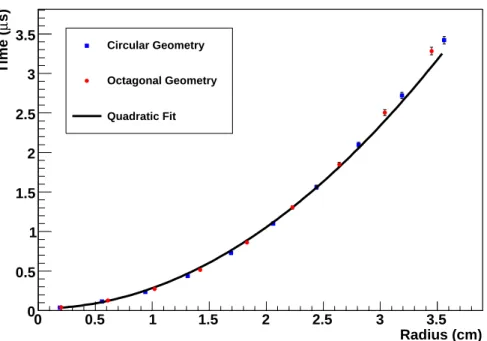
60
of the solar neutrino flux for these phases have been reported elsewhere [8, 9, 10, 11, 12, 13, 14].
61
3. Muon Reconstruction with the SNO Detector
62
The SNO muon reconstruction algorithm fits for a through-going muon track based on the
63
charge, timing, and spatial distribution of triggered PMTs. Using a maximum likelihood method,
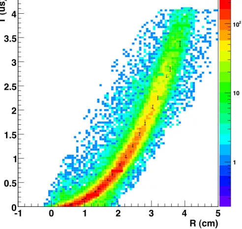
64
the fitter is able to determine a variety of muon tracking parameters, including the muon’s
propa-65
gation direction, impact parameter with respect to the center of SNO, the total deposited energy,
66
and a timing offset. The likelihood is defined as:
67 L= PMT s Y i ∞ X n=1 PN(n|λi)PQ(Qi|n)PT(ti|n) (1)
where n is the number of detected photons, PN(n|λi) is the probability of n photoelectrons being
68
detected for λiexpected number of detected photoelectrons, PQ(Qi|n) is the probability of seeing
69
charge Qigiven n photon hits, and PT(ti|n) is the probability of observing a PMT trigger at time
70
tgiven n photon hits.
71
The heart of the fitter lies in the first probability term, which is calculated based on Monte
72
Carlo simulations. Muons were simulated at discrete impact parameter values with random
di-73
rections through the detector. These simulations were used to create lookup tables for how many
74
photoelectrons are expected to be detected by a PMT at a given position with respect to a muon
75
track with a given impact parameter.
76
The second term further refines the fit by including the charge information from the PMTs,
77
and allows an estimate of the total energy deposited by the muon, correcting for offline PMTs
78
and the neck of the detector. This probability was calculated by simulating multiple photon hits
79
on all of the PMTs in SNO. For a given number of photon hits, the resulting charge distribution is
80
modeled as an asymmetric Gaussian with the widths extracted from simulations. This fit model
81
agrees well with the simulations for many photon hits, and acceptably for few photon hits (see
82
Figure 1).
7 photoelectrons 20 photoelectrons
Charge (GSC)
Probability
0
0.005
0.01
0.015
0.02
0.025
0.03
0
5
10
15
20
25
30
Figure 1: The normalized PMT charge distribution measured in (scaled) pedestal-subtracted ADC charge for the case of 7 and 20 photoelectrons striking a single PMT. The smooth curve (red) indicates the prediction from the charge parameterization model used in the reconstruction.
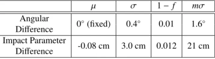
µ σ 1 − f mσ Angular 0◦(fixed) 0.4◦ 0.01 1.6◦ Difference Impact Parameter -0.08 cm 3.0 cm 0.012 21 cm Difference
Table 1: Accuracy of the muon fitter based on Monte Carlo simulations. Fit parameters for mean (µ), widths (σ and mσ), and relative weight (1 − f ) are given in Equations 4 and 5.
The third term in the likelihood refines the fit by including the PMT timing. For each PMT,
84
the time residual can be calculated as:
85 tres= tPMT,i− t0− d1 c − d2 cD (2)
where tPMT,iis the recorded time on a given PMT, t0is the time offset term in the likelihood fit,
86
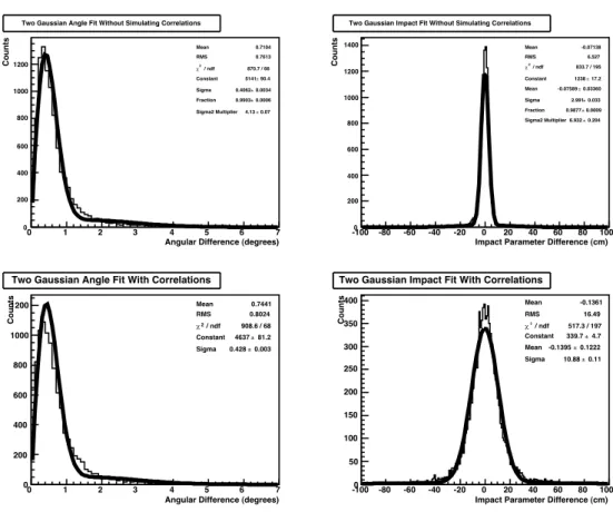
d1is the distance the muon travels within the detector before emitting the Cherenkov photon, c
87
is the speed of light in vacuum, d2is the distance the Cherenkov photon traveled, and cDis the
88
average speed of light in D2O/H2O medium (21.8 cm/ns). The Cherenkov photon is assumed
89
to have an angle of 42◦ with respect to the muon track, making d
1 and d2 well-defined. The
90
probability of the time residual is modeled as a Gaussian centered at zero with corrections to
91
include estimates of prepulsing and late light as a function of the number of photon hits.
92
The SNO muon fitter maximizes the likelihood function for the impact parameter, direction,
93
deposited energy, and timing offset using the method of simulated annealing with downhill
sim-94
plex [16]. After determining the parameters that maximize the likelihood, a set of data quality
95
measurements are used for background rejection.
96
The muon fitter is found to have good reconstruction accuracy for simulated muons.
Fig-97
ure 2 shows the angle (θmr) between the Monte Carlo generated muon direction (~ug) and the
98
reconstructed muon direction (~ur):
99
θmr= cos−1(~ug·~ur) (3)
This is fit to a weighted double Gaussian function:
100 p(θ)= Aθ " f e−2σ2θ2 + (1 − f )e− θ2 2(mσ)2 # (4) The additional θ-dependence is introduced in order to account for the phase space available.
101
The fit parameters are summarized in Table 1. Although the tails are non-Gaussian, this fit
102
gives a reasonable estimate for the uncertainty in the angular resolution. Figure 3 shows the
103
impact parameter reconstruction accuracy. The distribution is fit to the sum of two Gaussians:
104 p(x)= A " f e−(x−µ)22σ2 + (1 − f )e− (x−µ)2 2(mσ)2 # (5) with the fit parameters also summarized in Table 1. Monte Carlo studies show that the
recon-105
struction accuracy of the muon direction and impact parameter are uncorrelated.
Angular
Difference
(degrees)
0
1
2
3
4
5
6
7
Counts
0
200
400
600
800
1000
1200
Figure 2: The angular difference (as defined in Eq. 3) of Monte-Carlo muon tracks through the SNO detector (solid histogram). The angular distribution is fit to the function outlined in Eq. 4 (solid line). The results from the fit are given in Table 1.
Impact Parameter
Difference
(cm)
−40
−30
−20
−10
0
10
20
30
40
Counts
0
200
400
600
800
1000
Figure 3: The impact parameter difference of Monte-Carlo muon tracks through the SNO detector (solid histogram). The distribution is fit to the function outlined in Eq. 5 (solid line). The results from the fit are given in Table 1.
Scintillator P
anels
PMTsWire ChambersWire Chambers (X Plane) (Y Plane)
Mounting F rame
Wire Chamber 1 of 128 Bicron BC412151 Scintillator Photonis XP2262 PMT 1 of 3 per panel 1 of 4 1 of 4 per panel Photonis XP2262 PMT ECL – NIM – ECL Converter LeCroy 2132 HV‐CAMAC Interface Weiner CC32 CAMAC Controller Mac Computer running the
ORCA
data acquisiIon applicaIon LeCroy HV4032A High Voltage DistribuIon System FEE 1 per channel Discriminator LeCroy 3377 TDC LeCroy 2249A ADC HV4. The External Muon System
107
The External Muon System consists of a series of 128 single-wire chambers arranged into
108
four planes and triggered by three large scintillator panels (see Figure 4). The wire chamber cells
109
and electronics were provided by Indiana University. Each cell is 7.5 cm wide and has a square
110
cross-section with the corners trimmed into a near-octagonal shape. The cells are 2.564 m in
111
length and possess a single 50 µm diameter tungsten wire running through the center. The wire
112
is held at a positive potential of 2500 V (2700 V) while running on the surface (underground)
113
for electron drift and collection. A gas mixture of 90%Ar-10%CO2was used in order to achieve
114
high efficiency and stability, and to meet safety regulations for underground operations.
115
When a muon passes through the system, it deposits energy in the scintillator and ionizes
116
atoms in each of the wire chambers it passes through. The scintillator converts the energy into
117
light that is then detected by PMTs in a fast process (∼ns). In the wire chambers, the high voltage
118
draws the ionization electrons to the wire in a slow drift process (∼ µs). The drift time is
propor-119
tional to the closest distance between the muon track and the wire, allowing track reconstruction
120
using timing and position. The measured drift time for each wire is the time difference between
121
when the scintillator fired and when the drift electrons reached the wire.
122
The scintillator consists of three large rectangular panels (350 × 70 × 5 cm3) which cover
123
the active region of the EMuS detector. The panels were acquired from the KARMEN neutrino
124
experiment [17], and consisted of Bicron BC412 scintillator read out at each end by four
Photo-125
nis XP2262 PMTs. The signals from the PMTs were sent to a LeCroy 2249A Analog to Digital
126
Converter (ADC) and a discriminator. If both ends of a panel fire in coincidence, a start signal
127
was sent to the wire readout modules, and the ADC modules recorded the pulse-height of each
128
PMT.
129
Each wire chamber was monitored by an individual Front-End Electronics (FEE) card which
130
output an ECL signal if a pulse is detected on the wire. The ECL signal was sent to a LeCroy 3377
131
Time to Digital Converter (TDC) with a readout window of 4.1 µs. In order to mitigate high levels
132
of electronic noise in the pre-amplifiers, the readout cables were sent through an additional
ECL-133
NIM-ECL converter (see Figure 5).
134
The EMuS system was deployed on the deck of the SNO experiment, 12 m above and 3 m
135
west of the center of the detector. Due to space and solid-angle considerations, the planes were
136
inclined at a 55◦from horizontal. A survey was performed to determine the position of each of the
137
wires with respect to the SNO detector. The dominant sources of uncertainty associated with the
138
wire positions relative to the SNO detector are summarized in Table 2. The largest uncertainty
139
stems from determining X-Y coordinates of the EMuS detector. By comparing survey results
140
with other known location markers at the detector, the X-Y coordinate was determined to better
141
than ±0.53 cm. The reference point used for the Z-coordinate of the detector was only known
142
to ±0.32 cm, and thus added as an uncertainty to the EMuS location. Other uncertainties on the
143
locations of the wires included uncertainties on the floor level, the placement of the wires within
144
the modules, the spacing between wires, and the gaps between the modules. These additional
145
uncertainties do not apply equally to all wires, and have a maximum combined value of ±0.30 cm.
146
The final uncertainty on the SNO-EMuS coordinate translation based on this survey was ±0.68
Radius (cm) 0 0.5 1 1.5 2 2.5 3 3.5 s) µ Time ( 0 0.5 1 1.5 2 2.5 3 3.5
Circular Geometry
Octagonal Geometry
Quadratic Fit
Figure 6: The drift time for simulated electrons inside the EMuS wire chambers plotted as a function of starting radius. The plot shows drift times for both circular (boxes) and octagonal (circles) cross-sectional geometries. The quadratic fit (solid line) is accurate to within 5% at the maximum simulated radius.
closest approach of the muon. This time-to-radius conversion function, r(t), has been simulated
152
and measured for the EMuS system.
153
The Garfield gas simulation [19] was used to generate expected r(t) curves as a function of
154
gas pressure and applied voltage. The code was not able to perfectly model the shape of the wire
155
chambers so two similar geometries were used to check the effects of this imperfect modeling:
156
a circle with radius 3.75 cm, and a regular octagon with a longest radius of 4.06 cm. Simulated
157
electrons were generated at 10 points along the longest radius, and the mean drift time for each
158
point was calculated. Figure 6 shows that the two r(t) curves agree to within 2%. A parabolic fit
159
to this data is accurate to 5%.
160
In order to directly measure the r(t) curve, the EMuS system was run on the surface at the
161
SNO X-Y Coordinate 0.53 cm
SNO Z Coordinate 0.32 cm
Floor Level* 0.17 cm
Wire Placement 0.08 cm
Wire Spacing* 0.18 cm
Gaps Between Modules* 0.14 cm
Time to Radius Conversion 0.28 cm
Overall 0.74 cm
MIT-Bates Linear Accelerator Center in Middleton, MA. Candidate muon tracks are selected if
162
they pass through two adjacent chambers on two parallel planes. A series of data cleaning cuts
163
are applied to remove hit pairs created by noise and accidental triggers. Since the positions of
164
the wire chambers that fire are known, an estimate of the angle of the muon trajectory (θ) can be
165
calculated. Once the angle is known, the radii of closest approach are related as:
166
R1+ R2= D cos θ (6)
where D is the distance between each wire. A trial r(t) function (ρ(t)= at2+b) is used to estimate
167
R2as a function of the time from the other chamber:
168
R02= D cos θ − ρ(t1) (7)
A least-squared parameter B is constructed
169
B= (ρ(t2) − R02)
2 (8)
and then minimized. The resulting r(t) curve is shown in Figure 7. Slices in time show a Gaussian
170
shape, where the maximum width of these slices is 0.24 cm, which is taken as the uncertainty on
171
the time-to-radius conversion. The fit also extracts a negative time offset of 70 ns, which is caused
172
by delays introduced by the electronic signal chain. This time offset slightly decreases the
effi-173
ciency for reconstructing events, but does not significantly change the reconstruction accuracy.
174
Running conditions varied slightly between Bates lab and underground at SNO (mainly due to
175
ambient pressure and operating voltage) and simulations were used to correct for these changes.
176
The extrapolation provides an additional uncertainty of ±0.14 cm, yielding a total uncertainty of
177
±0.28 cm on the time-to-radius conversion model.
178
5. Data Selection
179
A number of data quality checks were made to find candidate muons that went through both
180
SNO and the EMuS system. Six of the EMuS wires were removed from the analysis because of
181
their abnormally low or high trigger rates. A small number of channels had multiple recorded
182
hits in a single event. For such events, only the first hit in time was considered part of the muon
183
track reconstruction algorithm.
184
EMuS event level cuts were defined to select muon events throughout the run of the
experi-185
ment. A minimum of three wire planes had to fire in order to ensure proper reconstruction. The
186
event also had to have fewer than 30 wires fired so as to reduce contamination from electrical
187
pickup. Finally, runs with increased human activity above the detector, due to calibrations or
188
source manipulation runs, were removed from the data analysis. A total of 62 EMuS events
189
passed all run selection criteria.
190
To correlate these candidate events with the SNO detector, all of the relevant SNO runs were
191
examined with an event viewer. Of the 62 EMuS events, 32 corresponded to a muon track passing
192
R (cm)
-1
0
1
2
3
4
5
T (us)
0
0.5
1
1.5
2
2.5
3
3.5
4
1 10 2 10Figure 7: Drift time as a function of radius for data taken at Bates Laboratory (surface measurement). The color axis indicates the number of events that reconstruct with the given radius and time. The vertical error bars are Garfield simulations of the drift time.
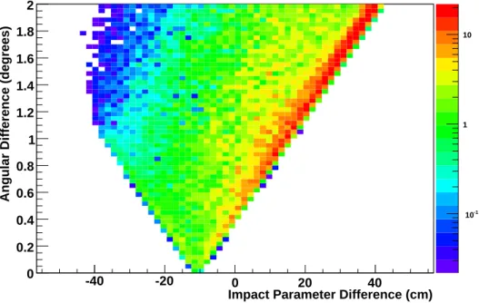
Impact Parameter Difference (cm) -40 -20 0 20 40 Angular Di fference (degrees) 0 0.2 0.4 0.6 0.8 1 1.2 1.4 1.6 1.8 2 -1 10 1 10
Figure 8: Angular difference vs impact parameter difference between SNO’s muon fitter and the EMuS system for one event. The color scale indicates the density of possible tracks weighted by their likelihood.
6. EMUs Reconstruction
199
By utilizing tracks that reconstruct in both SNO and the EMuS system, one can determine
200
the final muon track reconstruction accuracy. A Monte Carlo-based method is used to determine
201
such reconstruction characteristics. For each real data event that is reconstructed in both the SNO
202
and EMuS detector, a series of random test tracks are generated. These Monte Carlo generated
203
random tracks use the muon track as reconstructed by the SNO detector alone as a seed track, but
204
its vertex and direction are allowed to vary; with up to δθ ≤ 10◦variations in reconstruction angle
205
and up to δbµ ≤ 100 cm variations in impact parameter. Subsequently, these generated Monte
206
Carlo tracks are then compared to the hit pattern as recorded in the EMuS tracking chamber. The
207
negative log likelihood value (hereafter referred to as the likelihood) for each generated track is
208
calculated to determine the overall compatibility of the SNO muon reconstruction algorithm with
209
tracks reconstructed in the EMuS system. The likelihood is given by the following functional
210 form: 211 L= X wires i [bi−ρ(ti)]2 σ2 i (9)
where biis the impact parameter between the simulated track and the ithwire, ρ(ti) is the expected
Angular Difference (degrees) 0 1 2 3 4 5 6 7 Counts 0 200 400 600 800 1000 1200
Two Gaussian Angle Fit Without Simulating Correlations
Mean 0.7104 RMS 0.7613 / ndf 2 r 870.7 / 66 Constant 5141 ± 90.4 Sigma 0.4062 ± 0.0034 Fraction 0.9903 ± 0.0006 Sigma2 Multiplier 4.13 ± 0.07
Two Gaussian Angle Fit Without Simulating Correlations
Impact Parameter Difference (cm)
-100 -80 -60 -40 -20 0 20 40 60 80 100 Counts 0 200 400 600 800 1000 1200 1400
Two Gaussian Impact Fit Without Simulating Correlations
Mean -0.07138 RMS 6.527 / ndf 2 r 833.7 / 195 Constant 1238 ± 17.2 Mean -0.07589 ± 0.03360 Sigma 2.991 ± 0.033 Fraction 0.9877 ± 0.0009 Sigma2 Multiplier 6.932 ± 0.204
Two Gaussian Impact Fit Without Simulating Correlations
Angular Difference (degrees)
0 1 2 3 4 5 6 7 Counts 0 200 400 600 800 1000 1200
Two Gaussian Angle Fit With Correlations
Mean 0.7441 RMS 0.8024 / ndf 2 r 908.6 / 68 Constant 4637 ± 81.2 Sigma 0.428 ± 0.003
Two Gaussian Angle Fit With Correlations
Impact Parameter Difference (cm)
-100 -80 -60 -40 -20 0 20 40 60 80 100 Counts 0 50 100 150 200 250 300 350 400
Two Gaussian Impact Fit With Correlations
Mean -0.1361 RMS 16.49 / ndf 2 r 517.3 / 197 Constant 339.7 ± 4.7 Mean -0.1395 ± 0.1222 Sigma 10.88 ± 0.11
Two Gaussian Impact Fit With Correlations
Figure 9: Results from fitting the angular (left) and impact parameter (right) distributions of the ensemble of the gen-erated simulated data sets according to Equations 4 and 5; respectively. The top plots show the results of fitting the distributions directly from SNOMAN Monte Carlo simulation package without taking into account correlations between angle and impact parameter reconstruction in the EMuS data. The bottom plots show the results with the inclusion of these correlations.
Angular Difference (degrees) 0 1 2 3 4 5 6 7 Counts 0 1 2 3 4 5 6 7 Angular Fit χ2 / ndf 9.281 / 26 Constant 17.26 ± 4.66 Sigma 0.6135 ± 0.0622 Angular Fit
Impact Parameter Difference (cm)
−100 −80 −60 −40 −20 0 20 40 60 80 100 Counts 0 1 2 3 4 5 6
Impact Parameter Fit χ2 / ndf 18.37 / 47
Constant 2.406 ± 0.583
Mean 4.261 ± 3.749
Sigma 18.59 ± 2.98
Impact Parameter Fit
Figure 10: Gaussian fit to the data jointly reconstructed by the EMuS-SNO systems. Figure shows both angular (left) and impact parameter (right) difference.
reconstructed by the EMuS system. This is expected because if the track direction is changed
218
(raising the angular difference) the placement of the track can be changed (raising the impact
219
parameter difference) without significantly altering the hit pattern recorded by the EMuS system.
220
Since this ambiguity exists only in the EMuS system and not in SNO’s muon tracking
algo-221
rithm, we can compare tracks reconstructed in the two systems by assuming either (a) the impact
222
parameter is fixed or (b) the reconstructed track direction is fixed. To test the validity of these
223
assumptions, an ensemble of fake data sets is generated both with and without accounting for
224
track correlations in the EMuS system. The results from these Monte Carlo tests are shown in
225
Figure 9. Correlations have no effect on the angular mis-reconstruction or the means of the
distri-226
butions, but they do broaden the impact parameter mis-reconstruction by as much as 10 cm. We
227
conclude that the EMuS-SNO tracks are sensitive enough to constrain the angular
reconstruc-228
tion and impact parameter bias of the SNO muon fitting algorithm, but not the resolution of the
229
impact parameter reconstruction.
230
Figure 10 shows the results of applying the two assumptions to the 30 reconstructed
EMuS-231
SNO events. The data are fitted to the functional forms of Equations 4 and 5. Due to the small
232
number of events, the weights and relative widths of the secondary gaussians are fixed to their
233
values from the earlier simulations. We find that the angular width is 0.61◦± 0.06◦. The impact
234
parameter bias is 4.2 ± 3.7 cm, while fit impact parameter width is 18 ± 11 cm.
235
7. Conclusions
236
The combined data from the SNO detector and the External Muon System have demonstrated
237
that the SNO muon reconstruction algorithm is accurate to the level needed by the
neutrino-238
induced atmospheric flux analysis. The EMuS analysis places a constraint on the angular
recon-239
struction to better than 0.61◦± 0.06◦and on the impact parameter bias to better than 4.2 ± 3.7 cm.
240
The latter constraint is in good agreement with other methods using cosmic-ray data in SNO [1].
241
8. Acknowledgements
244
This research was supported by: Canada: Natural Sciences and Engineering Research
Coun-245
cil, Industry Canada, National Research Council, Northern Ontario Heritage Fund, Atomic
En-246
ergy of Canada, Ltd., Ontario Power Generation, High Performance Computing Virtual
Labora-247
tory, Canada Foundation for Innovation; US: Dept. of Energy, National Energy Research
Sci-248
entific Computing Center; UK: Science and Technology Facilities Council; Portugal: Fundac¸˜ao
249
para a Ciˆencia e a Tecnologia. We would like to thank Indiana University, Los Alamos National
250
Laboratory, and K. Eitel for loan of equipment to make the measurement possible. We would
251
also like to thank the SNO technical staff for their strong contributions and Vale (formerly Inco)
252
for hosting this project.
253
[1] B. Aharmim et al., Phys. Rev. D 80 (2009) 012001.
254
[2] Y. Ashie et al., Phys. Rev. D 71 (2005) 112005.
255
[3] P. Adamson et al., Phys. Rev. D 77 (2008) 072002.
256
[4] B. A. Moffat et al., Nucl. Instrum. Meth. A 554 (2005) 255.
257
[5] G. Doucas et al. Nucl. Instrum. Methods A 370:579 (1996).
258
[6] J. Boger et al., Nucl. Instrum. Meth. A 449 (2000) 172.
259
[7] M. R. Dragowsky et al., Nucl. Instrum. Meth. A 481 (2002) 284.
260
[8] Q.R. Ahmad et al., Phys. Rev. Lett. 87 (2001) 071301.
261
[9] Q.R. Ahmad et al., Phys. Rev. Lett. 89 (2002) 011301.
262
[10] Q.R. Ahmad et al., Phys. Rev. Lett. 89 (2002) 011302.
263
[11] B. Aharmim et al., Phys. Rev. C 75 (2007) 045502.
264
[12] S.N. Ahmed et al., Phys. Rev. Lett. 92 (2004) 181301.
265
[13] B. Aharmim et al., Phys. Rev. C 72 (2005) 055502.
266
[14] B. Aharmim et al., Phys. Rev. Lett. 101 (2008) 11130.
267
[15] M.A. Howe et al., IEEE Trans. Nucl. Sci. 51 (2004) 878.
268
[16] W. H. Press, S. A. Teukolsky, W. T. Vetterling, and B. P. Flannery, Numerical Recipes in Fortran, Cambridge
269
University Press, 2nd ed (1992).
270
[17] H. Gemmeke et al., Nucl. Instrum. Meth. A 289, 490 (1990).
271
[18] A. Peisert and F. Sauli, CERN-84-08 (1984).
272
[19] R. Veenhof, “Garfield”, CERN Program Library (1998).