Publisher’s version / Version de l'éditeur: Proceedings, 2003
READ THESE TERMS AND CONDITIONS CAREFULLY BEFORE USING THIS WEBSITE.
https://nrc-publications.canada.ca/eng/copyright
Vous avez des questions? Nous pouvons vous aider. Pour communiquer directement avec un auteur, consultez la
première page de la revue dans laquelle son article a été publié afin de trouver ses coordonnées. Si vous n’arrivez pas à les repérer, communiquez avec nous à PublicationsArchive-ArchivesPublications@nrc-cnrc.gc.ca.
Questions? Contact the NRC Publications Archive team at
PublicationsArchive-ArchivesPublications@nrc-cnrc.gc.ca. If you wish to email the authors directly, please see the first page of the publication for their contact information.
NRC Publications Archive
Archives des publications du CNRC
This publication could be one of several versions: author’s original, accepted manuscript or the publisher’s version. / La version de cette publication peut être l’une des suivantes : la version prépublication de l’auteur, la version acceptée du manuscrit ou la version de l’éditeur.
Access and use of this website and the material on it are subject to the Terms and Conditions set forth at
The Friction Coefficient of a Large Ice Block on a Sand/Gravel Beach
Timco, Garry; Barker, Anne
https://publications-cnrc.canada.ca/fra/droits
L’accès à ce site Web et l’utilisation de son contenu sont assujettis aux conditions présentées dans le site LISEZ CES CONDITIONS ATTENTIVEMENT AVANT D’UTILISER CE SITE WEB.
NRC Publications Record / Notice d'Archives des publications de CNRC:
https://nrc-publications.canada.ca/eng/view/object/?id=e7337f27-5c6b-4074-9866-9b2d83ae341b https://publications-cnrc.canada.ca/fra/voir/objet/?id=e7337f27-5c6b-4074-9866-9b2d83ae341b
CGU HS Committee on River Ice Processes and the Environment
12th Workshop on the Hydraulics of Ice Covered Rivers
Edmonton, AB, June 19-20, 2003
The Friction Coefficient of a Large Ice Block on a Sand/Gravel Beach
Anne Barker and Garry Timco
Canadian Hydraulics Centre
National Research Council of Canada, Ottawa, Ont. K1A 0R6 anne.barker@nrc-cnrc.gc.ca, garry.timco@nrc-cnrc.gc.ca
The amount of ice ride-up on beaches and shorelines is a function of the slope of the beach, the driving force, the size of the ice blocks, and the friction between the ice and the beach. Predicting the amount of ride-up is difficult, primarily because little is known about the friction coefficient of large ice blocks on sand/gravel beaches. To investigate this, a test program was performed to measure the friction of a large block of ice sliding on a sand/gravel beach. Four different friction coefficients were measured, corresponding to the four modes of movement of the block on the beach: static, bulldozing, transition and sliding. The friction coefficient decreased as the movement mode changed from static to sliding. The statistical analysis of the friction coefficient values showed that the mean value generally decreased with an increase in velocity. The static friction values were approximately the same for each test. The results of these tests will be presented in this paper, as well as a discussion of the implications of the results on the ride-up processes of ice on these types of shorelines.
1. Introduction
Ice ride-up and pile-up has been discussed extensively in the ice-related literature (see e.g. Kovacs and Sodhi 1980, 1988; Kovacs 1983, 1984; Croasdale et al 1988; Christensen 1994; Timco and Barker 2002). In certain situations it is important to be able to predict if ice pile-up or ride-up will occur. Several factors influence ride-up and pile-up events including the thickness, strength and size of the ice floe, the local geometry and roughness of the shore, the driving force on the floe, the initial size and velocity of the floe, and the friction coefficient between the ice and the shoreline soil. In most situations, all of these factors can be quantified except for the friction coefficient between the ice and shoreline soil. Since very little quantitative information is known about this, a test program was carried out to measure the friction coefficient between a large block of ice and a sand/gravel mix. The tests were carried out using a large block of ice that would be representative of a typical ice block in nature. The test procedure and results are presented in this paper.
2. Test Set-Up
2.1 Test Facility
The tests were performed in the ice tank at the NRC Canadian Hydraulics Centre (CHC) in Ottawa (Pratte and Timco, 1981). The tank is 21 m long by 7 m wide and 1.2 m deep, and is housed in a large insulated room that can be cooled down to an air temperature of -20°C. A carriage that can travel the length of the tank spans the tank. The carriage is driven through two helical-cut rack and pinion gears, and is designed for loads up to 50 kN with a speed range from 0.003 to 0.65 m/s. A smaller service carriage also spans the tank. For these tests, the main carriage was driven backwards along the tank, pulling the ice block behind it. During a test, the output from the instrumentation was sampled, digitized and stored for subsequent analysis and computation.
2.2 Seabed
The soils used in this study consisted of a fine, well-graded gravel and a coarse, well-graded sand. These two materials were mixed together at an approximate ratio of 1 part sand to 2/3 part gravel at the start of the testing program. The sand and gravel were placed in the ice tank by a loader in the dry. This material was placed in approximately 0.15 m lifts. As each lift was placed, some water was added to facilitate packing. Packing was performed on each lift using a vibratory plate compactor. Once the material had been sufficiently compacted to achieve a consistent, high placement density, the chamber was then cooled to a temperature of +2°C. After each test, the sand/gravel mix that was disturbed was raked back into place. There were two sections of the channel – one where the sand/gravel mix was smooth, and another where it was rough, in order to examine the differences between the two.
2.3 Ice block
The ice block was built up in a two-part plywood mold (Figure 1) in the CHC cold room. The mold’s outside dimensions were 0.8 m x 0.8 m x 0.76 m. The freshwater ice used in the block was initially frozen in plastic tubs. Once frozen, this ice was broken up using a 2 lb sledgehammer, into chunks with diameter generally less than 0.1 m. The ice was added to the
mold in 0.05 m layers, as a slurry, using chilled water. Midway up the mold, strapping was frozen in place in order to facilitate lifting the ice block with a forklift and a jib crane. After the final layer was added and frozen, the top of the ice block was smoothed using a palm sander. Before testing, the lower plywood mold was removed to expose the ice. A hole was drilled through the ice block and plywood mold at the centre of buoyancy. A 5/8” metal rod was inserted, and an eyebolt was attached at one end, with a metal plate at the other end, so that the main carriage could tow the block. The back of the ice block, with the plywood bottom removed, is shown in Figure 2. The dimensions of the block were 0.72 m x 0.72 m x 0.70 m. The mass of the ice block, with the wooden top attached, was approximately 400 kg. The average footprint pressure was calculated as approximately 7 kPa.
Figure 2 Back of ice block with plywood top and towing plate
2.4 Instrumentation
A 6-component dynamometer, composed of six Interface load cells mounted in different configurations, was used to measure the applied ice loads (Figure 3). The dynamometer consists of three load cells mounted to measure forces in the z-direction, two in the x-direction and one in the y-direction. The instrumentation was calibrated to ensure reliable and accurate performance prior to installation in the ice tank. Factory calibration constants were used for the dynamometer since in situ calibration was not possible. However, these factory constants were verified by a number of static tests.
The data acquisition system (DAS) recorded the analogue signals from the instrumentation. The signals were sampled and digitized by a NEFF Instruments System 100 data acquisition system. The data was sampled at a rate of 100 Hz. During sampling, an analogue low-pass filter with a cut-off frequency of 33 Hz was applied to prevent aliasing. The digitized signals were recorded on a Digital VAX AlphaStation computer as GEDAP data files (Miles, 1990). GEDAP is a software package developed at the CHC to facilitate experiment control, data acquisition, data analysis and the graphical presentation of time series data.
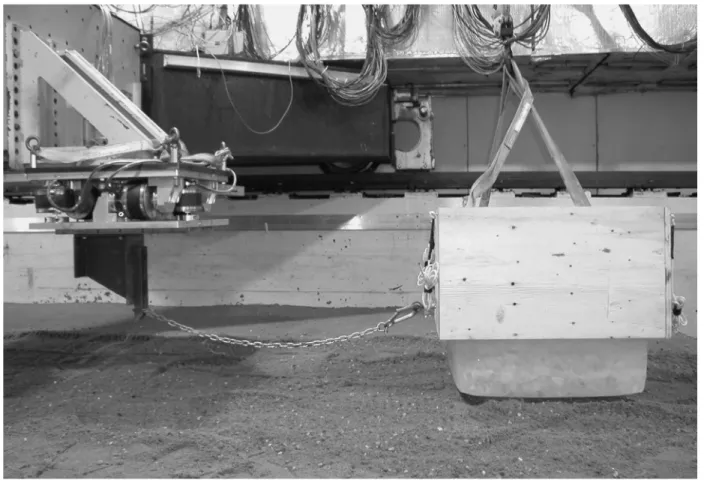
Figure 3 shows the overall set-up for the test series. A 0.37 m-long bracket that had an eyebolt inserted at its base was attached underneath the Dynamometer. A 1 m-long, lightweight chain was then attached with shackles to both the bracket and to the eyebolt on the block for towing. The block was brought from the cold room to the environmental chamber using a forklift. The instrumentation was re-zeroed before each test with everything held stationary. When this was completed, the DAS was started, and the ice block was pulled along the bed material at the
desired velocity. The carriage was stopped after it had travelled the length of the channel, and then the DAS system was also stopped. The ice block was lifted using a jib crane, and the entire set-up was moved back to the beginning of the test channel. The seabed material was then raked back into place. Six tests were performed at different velocities.
Figure 3 Test set-up. The six-component dynamometer and towing bracket are on the left. 3. Results
After testing was complete, the six channels of recorded data were transferred to a PC, where the sum of the forces in the x-direction was calculated. This data set was then transformed into a time-series of the friction coefficient, by dividing the sum-Fx time-series by 3.9 kN, which was
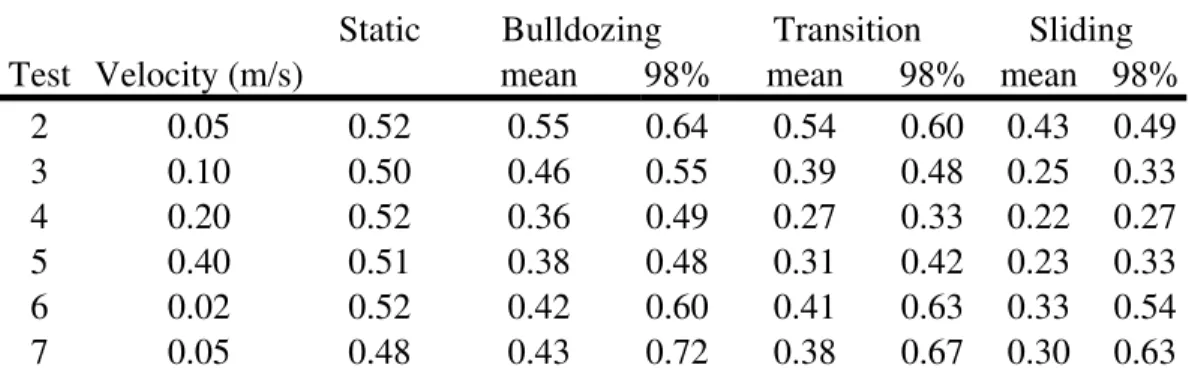
the weight of the block. The test matrix and results are shown in Table 1. The first test in the series was discarded due to set-up difficulties. Visual observation of the tests indicated that, especially at the lower test velocities, the ice was moving in a stick-slip pattern.
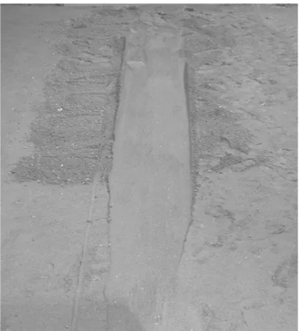
Figure 4 shows a typical time-series trace from a test. Statistical analysis of the data provided the mean and the 98% probability level value of the friction coefficient, taken over each of the three observed sections along the channel: a bulldozing section, along the rough section of the channel; a transition area where the ice block rode up out of the bulldozing trench it had created; and a surface sliding section along the smooth portion of the channel (see Figure 5). Additionally, the static friction coefficient was calculated from the initial force at the moment of contact between the ice and the seabed.
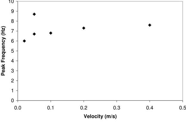
The statistical analysis of the friction coefficient values showed that the mean value generally decreased with an increase in velocity (Figure 6). The bulldozing section of the test channel had higher friction values than the surface sliding section. The static friction values were generally the same for each test, with a mean value of 0.50. Spectral analysis of the friction coefficient time series plots showed that the peak frequency of the time-series traces generally increased with increasing velocity (Figure 7).
Table 1 Test matrix and measured friction coefficient values
Static Bulldozing Transition Sliding
Test Velocity (m/s) mean 98% mean 98% mean 98%
2 0.05 0.52 0.55 0.64 0.54 0.60 0.43 0.49 3 0.10 0.50 0.46 0.55 0.39 0.48 0.25 0.33 4 0.20 0.52 0.36 0.49 0.27 0.33 0.22 0.27 5 0.40 0.51 0.38 0.48 0.31 0.42 0.23 0.33 6 0.02 0.52 0.42 0.60 0.41 0.63 0.33 0.54 7 0.05 0.48 0.43 0.72 0.38 0.67 0.30 0.63
Figure 4 Calculated friction coefficient value versus time for test #4
Static
Figure 5 Photograph of a scour path. The bulldozing section is at the top of the picture, followed by the transition to the surface sliding section of the test.
0.0 0.1 0.2 0.3 0.4 0.5 0.6 0.7 0.8 0 0.1 0.2 0.3 0.4 0.5
Velocity (m/s)
Friction Coefficient
Static Bulldozing Transition SlidingFigure 6 Plot of friction coefficients versus velocity. Static coefficient values were taken at the initiation of movement of the ice block over the sediment, while kinetic coefficient values are the mean value for each type of interaction (bulldozing, transition, sliding).
0 1 2 3 4 5 6 7 8 9 10 0.0 0.1 0.2 0.3 0.4 0.5 Velocity (m/s) Peak Frequency (Hz)
4. Discussion
4.1 Ice Friction Measurements On Various Materials
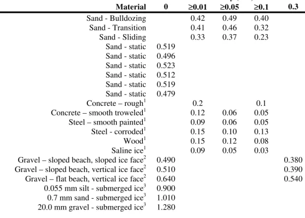
The results from this study were compared with previous laboratory and field studies examining ice friction. In Frederking and Barker (2001), the friction of sea ice on various materials such as smooth and rough concrete, rusted and smooth steel, wood and ice was investigated. The footprint pressure for the Frederking and Barker (2001) tests was either 65 kPa or 130 kPa, approximately 10 to 18 times higher than the present tests. The temperature of the ice was varied by changing the air temperature within the environmental chamber. The authors found that friction was higher at lower speeds and on rough materials, as may be expected. The average coefficient of friction of sea ice on smoother materials was found to be about 0.05 for speeds higher than 0.05 m/s and 0.1 at 0.01 m/s (Table 2). On rough materials, the average coefficient of friction was 0.1 at speeds greater than 0.1 m/s and increased to 0.2 at speeds around 0.01 m/s. They also observed weak trends of lower friction coefficient at higher contact pressures and higher friction coefficient with higher temperatures. Values of the friction coefficient in the present study were larger than those measured by Frederking and Barker (2001). In the present study, deformation of the seabed occurred. This factor, combined with the force required to bulldoze the block of ice through the seabed material, could account for these high friction coefficient values.
A large-scale field study of the friction coefficient between gravel and ice was carried out by Shapiro and Metzner (1987). In their study, large blocks of sea ice were cut from a leading ice edge, then dragged either up or along a gravel beach by a bulldozer. These blocks were approximately 30 times more massive than the present study (ice block with vertical contact face: 3m x 3m x 1.2m; ice block with sloping contact face: 2.7 m x 2.2 m x 1.2 m), with a mean contact pressure of approximately 10 kPa and a density slightly higher than the ice blocks modeled here, primarily due to some gravel embedded near the top of the sea ice. The blocks were pulled with an approximate velocity of 0.3 m/s. The mean friction coefficient values from the Shapiro and Letzner study are also shown in Table 2. It can be seen that the values from this study are similar to the present investigation. In the Shapiro study, the authors investigated two types of ice blocks – one with a sloped face and one with a vertical face. The authors found that the difference in the shapes of the leading edge of the ice block were not important with respect to the friction coefficient of ice on a sloped gravel beach. They also noted that the friction coefficient was higher for the ice block towed along the vertical beach, compared to up the sloping beach (angle = 10°). They hypothesized that this could be because the beach might not have been completely flat. They noted that, for example, a 4° slope would decrease the friction coefficient by 0.07, using their formula for calculating the friction coefficient.
An additional set of tests performed by Utt and Clark (1980) were compared with the present study. In these tests, a block of ice was submerged using lead weights and towed along three different materials, as listed in Table 2, under different contact pressure conditions (all less than 4.6 kPa). The soil was smoothed for all cases. It can be seen that these test results were much higher than either the Shapiro or the present tests. Utt and Clark felt that the differences were accounted for by the lower contact pressures, smoothed surfaces and submerged test blocks in their study.
Table 2 Comparison of friction coefficients from laboratory and field studies Velocity (m/s) Material 0 ≥0.01 ≥0.05 ≥0.1 0.3 Sand - Bulldozing 0.42 0.49 0.40 Sand - Transition 0.41 0.46 0.32 Sand - Sliding 0.33 0.37 0.23 Sand - static 0.519 Sand - static 0.496 Sand - static 0.523 Sand - static 0.512 Sand - static 0.519 Sand - static 0.479 Concrete – rough1 0.2 0.1
Concrete – smooth troweled1 0.12 0.06 0.05
Steel – smooth painted1 0.09 0.06 0.05
Steel - corroded1 0.15 0.10 0.13
Wood1 0.15 0.12 0.08
Saline ice1 0.09 0.05 0.03
Gravel – sloped beach, sloped ice face2 0.490 0.380
Gravel – sloped beach, vertical ice face2 0.510 0.390 Gravel – flat beach, vertical ice face2 0.640 0.540
0.055 mm silt - submerged ice3 0.900
0.7 mm sand - submerged ice3 1.010
20.0 mm gravel - submerged ice3 1.280
1Frederking and Barker, 2001
2Shapiro and Metzner, 1987
3Utt and Clark, 1980
4.2 Implications For Ride-Up Measurements
Christensen (1994) discusses formulae for calculating the necessary forces for ice pile-up and ride-up initiation. For ice ride-up, he calculated that ride-up might occur when the available horizontal driving force’s component parallel to the slope is larger than the parallel resistance. This is calculated as ) tan (µ α γ + >L bh F i [1]
where F is the available horizontal driving force, L is the slope length above water covered by ice pieces, b is the width of ice on the slope, h is the ice sheet thickness, γi is the specific weight
of the ice, α is the slope angle and µ is the friction coefficient. Using this equation, a small parametric study was carried out, incorporating the measured mean friction coefficients (Table 1). The values for L, γi, b and h were held constant, while the friction coefficient and
slope of the beach changed. The results are shown in Table 3.
The table shows that changing the friction factor by approximately 0.1 changes the required force for ride-up by roughly 1 kN. Figure 8 and Figure 9 show these results in a graphical format.
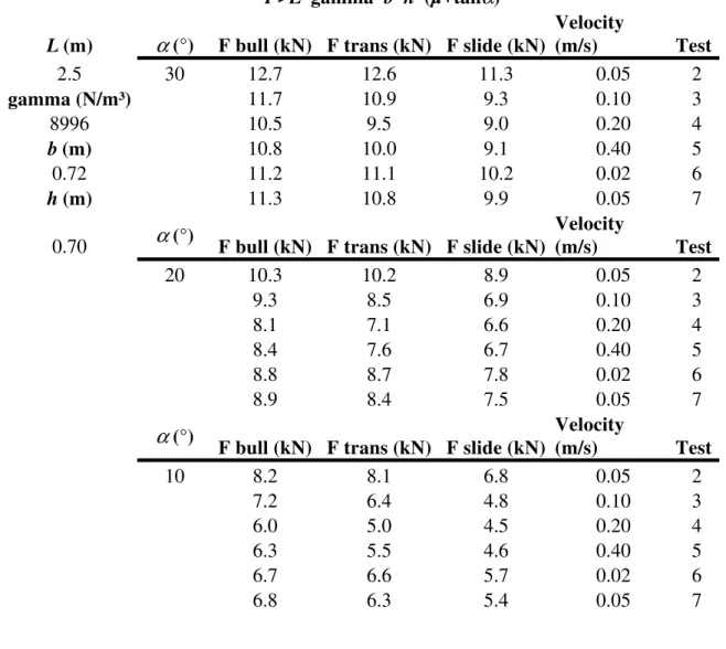
Table 3 Parametric study results
F>L*gamma*b*h*(µ+tanα)
L (m) α (°) F bull (kN) F trans (kN) F slide (kN)
Velocity (m/s) Test 2.5 30 12.7 12.6 11.3 0.05 2 gamma (N/m³) 11.7 10.9 9.3 0.10 3 8996 10.5 9.5 9.0 0.20 4 b (m) 10.8 10.0 9.1 0.40 5 0.72 11.2 11.1 10.2 0.02 6 h (m) 11.3 10.8 9.9 0.05 7
0.70 α (°) F bull (kN) F trans (kN) F slide (kN)
Velocity (m/s) Test 20 10.3 10.2 8.9 0.05 2 9.3 8.5 6.9 0.10 3 8.1 7.1 6.6 0.20 4 8.4 7.6 6.7 0.40 5 8.8 8.7 7.8 0.02 6 8.9 8.4 7.5 0.05 7 α (°)
F bull (kN) F trans (kN) F slide (kN)
Velocity (m/s) Test 10 8.2 8.1 6.8 0.05 2 7.2 6.4 4.8 0.10 3 6.0 5.0 4.5 0.20 4 6.3 5.5 4.6 0.40 5 6.7 6.6 5.7 0.02 6 6.8 6.3 5.4 0.05 7
0 2 4 6 8 10 12 14 0 0.1 0.2 0.3 0.4 0.5 Velocity (m/s) Force (kN) Slope = 30° Slope = 20° Slope = 10° Bulldozing
Figure 8 Bulldozing force required for pile-up with changing ice velocity and slope.
0 2 4 6 8 10 12 14 0 0.1 0.2 0.3 0.4 0.5 Velocity (m/s) Force (kN) Slope = 30° Slope = 20° Slope = 10° Sliding
Figure 9 Sliding force required for pile-up with changing ice velocity and slope.
It is possible to use Equation (1) to estimate the ride-up length on a beach for different shoreline slopes and ride-up behaviour. Consider the following example. An ice field extends 10 km outwards from a 1 km wide shore. The ice is pressed against the shore by winds averaging 20 m/s at 10 m height. The force (Fa) from the wind on the ice sheet is given by
2 v c A
Fa =ρ [2]
where ρ is the density of air, A is the horizontal area of the ice, and v is the wind speed measured at a height of 10 m. The corresponding drag coefficient (c) for smooth ice can be taken as
2 X 10⁻³ (Ashton, 1986). In this example, the area is 10 km2, and using c = 0.002, and an air density of 1.3 kg/m3, the total wind-drag force is approximately 10 MN.
Figure 10 shows the results for a case with an ice velocity at the shore of 0.2 m/s, the associated friction coefficient from Table 1, an ice thickness of 0.4 m, and using an assumption that the loading is uniform along the beach. In this example, the ride-up length was calculated for both bulldozing and sliding modes. The results show that the length of the ride-up decreases with increasing shoreline slope, as expected. Quantitative values show that, for ice sliding, the ride-up length can be on the order of 10 to 12 m for a relatively flat beach slope. If the ice block bulldozes, the ride-up length is lower, on the order of 7 m. This example illustrates that the mode of ice sliding can significantly affect the amount of ride-up especially for shallow beaches.
0 2 4 6 8 10 12 0 5 10 15 20 25 30
Slope of Shoreline (degrees)
Length of Ride-up (m)
Sliding
Bulldozing
Figure 10 Length of ride-up versus slope of shoreline. 5. Summary
A test program has been performed to measure the friction of a large block of ice sliding on a sand/gravel shore. Four different friction coefficients were measured corresponding to the four modes of movement of the block on the beach: static, bulldozing, transition and sliding. The friction coefficient decreased as the movement mode changed from static to sliding. The friction
coefficient was found to be a function of the velocity of the interaction and generally decreased with increasing velocity. The results of these tests demonstrate the direct implication on the amount of ride-up that could occur on beaches from ice pushing onto a beach with respect to the friction between ice and sand.
6. Acknowledgements
The support of the Program on Energy Research and Development (PERD) Ice-Structure Interaction Program Activity is gratefully acknowledged.
7. References
Ashton, G. D. 1986. River and Lake Ice Engineering. Water Resources Publications, Littleton, U.S.A.
Christensen, F.T. 1994. Ice Ride-up and Pile-up on Shores and Coastal Structures. Journal of Coastal Engineering Vol. 10, No. 3, pp 681-701.
Croasdale, K. R., Allyn, N. and Roggensack, W. 1988. Arctic Slope Protection: Considerations for Ice. In ASCE Arctic Coastal Processes and Slope Protection Design, edited by A.T. Chen and C.B. Leidersdorf. American Society of Civil Engineers, New York, N.Y., USA., pp 216 - 243.
Frederking, R. and Barker, A. 2001. Friction of Sea Ice on Various Construction Materials. PERD/CHC Report 3-49, HYD-TR-067. Ottawa, Canada.
Kovacs, A. 1983. Shore Ice Pile-up and Ride-up Features; Part 1: Alaska's Beaufort Sea Coast. U.S. Army CRREL Report 83-9, Hanover, N.H., USA.
Kovacs, A. 1984. Shore Ice Pile-up and Ride-up Features; Part 2: Alaska's Beaufort Sea Coast - 1983 and 1984. U.S. Army CRREL Report 83-9, Hanover, N.H., USA.
Kovacs, A. and Sodhi, D. 1980. Shore Ice Pile-up and Ride-up: Field Observations, Models and Theoretical Analysis. Cold Regions Science and Technology 2 , pp 209-288.
Kovacs, A. and Sodhi, D. 1988. Onshore Ice Pile-up and Ride-up: Observations and Theoretical Assessment. In ASCE Arctic Coastal Processes and Slope Protection Design, edited by A.T. Chen and C.B. Leidersdorf. American Society of Civil Engineers, New York, USA., pp 108 -142.
Miles, M.D., 1990. The GEDAP Data Analysis Software Package. NRC Report TR-HY-030. Ottawa, Canada.
Pratte, B.D. and Timco, G.W. 1981. A New Model Basin for the Testing of Ice-Structure Interactions. Proceedings 6th International Conference on Port and Ocean Engineering under Arctic Conditions, Vol. II, pp 857-866, Quebec City, Canada.
Shapiro, L.H. and Metzner, R.C. 1987. Coefficients of Friction of Sea Ice on Beach Gravel. Journal of Offshore Mechanics and Arctic Engineering, Vol. 109, pp. 388-390.
Timco, G. and Barker, A. 2002. What is the maximum pile-up height for ice? Proceedings 16th IAHR Symposium on Ice, Vol.2, pp.69-77, Dunedin, New Zealand.
Utt, M.E. and Clark, R.A. 1980. Coefficient of Friction Between Submerged Ice and Soil. American Society of Mechanical Engineers. Petroleum Division Journal, No.80-PET-41, p.1-4. United States.