Characterization and modeling of a 30 kilohertz transformer

Characterization and Modeling of a 30 Kilohertz

Transformer

by

Anne M. Mitzel

Submitted to the Department of Electrical Engineering and Computer

Science

in partial fulfillment of the requirements for the degree of

Master of Enineering in Electrical Science and Engineering

at the

MASSACHUSETTS INSTITUTE OF TECHNOLOGY

January 2001

37C4V

O t4109

©

Anne M. Mitzel, MMI. All rights reserved.

The author hereby grants to MIT permission to reproduce and

distribute publicly paper and electronic copies of this thesis document

in whole or in part.

JUL 112001

LIBRARIES

Department of Electrical Engineering and Computer Science

October 2, 2000

Certified by ...

...

...

...

Mouhoub Mekhiche, Ph.D.

Electro Magnetis/Mechanical roup Leader, Satcon Technology

Corporation 'I'he sSupeyvisor

Accepted by... ...-... ...

u

Ch , n C i n G.

Smith

Chairman,

Author.

Characterization and Modeling of a 30 Kilohertz

Transformer

by

Anne M. Mitzel

Submitted to the Department of Electrical Engineering and Computer Science on October 2, 2000, in partial fulfillment of the

requirements for the degree of

Master of Enineering in Electrical Science and Engineering

Abstract

A 30 kilohertz transformer for a power conditioning unit was characterized through

ex-tensive experimental measurements. Measurements of the driving-point impedance of the transformer were used to create an equivalent circuit model of the transformer, and the model was optimized for close correspondence between the measured impedance and the impedance of the equivalent circuit. While the impedance predicted by the model bore a close resemblance to the actual driving point impedance of the trans-former, the model was unable to predict the transient behavior of the transformer in its operational environment. The model was evaluated to be an impractical method of simulating transformer behavior in a power electronics circuit.

Thesis Supervisor: Jeffrey H. Lang Title: Professor, EECS

Thesis Supervisor: Mouhoub Mekhiche, Ph.D.

Acknowledgments

I would like to thank Mouhoub Mekhiche at SatCon for his invaluable help throughout this project. I would also like to thank Evgeny Holmansky at SatCon for providing the data for the transformer and Professor Lang for his advice and help.

Contents

3.1 Equivalent circuit model . . . .

3.2 Experimental measurements . . . .

3.2.1 Configuration BD . . . .

3.2.2 Configuration AB CD . . . . .

3.2.3 Configurations AC, BC, and AD 3.2.4 Equipment . . . .

4 Identification of the Equivalent Circuit

4.1 Modification of the equivalent circuit . 4.1.1 Coupling coefficient . . . . 4.1.2 Loss parameters . . . . 4.2 Optimization procedure . . . .

4.3 Calculation of six capacitor values . . . 5 Simulation

5.1 Sim ulation tool . . . .-. . . . .

5.2 The transformer as a stand-alone circuit . . . .

9 10 13 16 19 . . . . 19 . . . . 22 . . . . 23 . . . . 26 . . . . 26 . . . . 27 Parameters 29 . . . . 30 . . . . 32 . . . . 33 . . . . 34 . . . . 37 40 40 41

5.3 The transformer in its operational environment . . . . 5.3.1 Transient simulation results . . . .

6 Results and Conclusions

6.1 Interpretation of results . . . . 6.2 C onclusion . . . .

A Maple Code

A.1 Short-circuit impedance . . . . A.2 Open-circuit impedance . . . . A.3 Open-circuit resonant frequencies . . . .

B Matlab Scripts

B.1 Minimization script for inductances, B.1.1 lxiter.m . . . . B.1.2 reserr.m . . . . B.1.3 reserrsimpl.m . . . . B.1.4 magnerr.m . . . . B.1.5 finaldrivingpoint.m... B.1.6 finaldrivingcc.m . . . . B.2 Determination of six capacitors . .

C Equivalent Model for Remaining

C.1 Measured Data . . . .

C.2 Equivalent Circuit Model . . . .

capacitances, and resistances

Transformer Configurations . . . . . . . . 47 50 58 58 59 62 62 64 68 72 72 72 76 77 79 80 83 85 93 93 97

List of Figures

1-1 DC to DC converter ... ...

1-2 Connections to primary and secondary windings . . . . .

1-3 Magnetic structure of transformer . . . . 1-4 Block diagram of procedure . . . .

11 11 12 14

Equivalent circuit model of transformer . . . . 20

Three independent voltages of a two-winding transformer . . . . 20

Six capacitors of the equivalent circuit model . . . . 21

Impedance of secondary, primary open . . . . 23

Impedance of secondary, primary shorted . . . . 24

Impedance of primary, secondary open . . . . 25

Simplified equivalent circuit model of the transformer . . . . 30

Simplified circuit with additional inductance . . . . 31

Simplified circuit with additional inductance . . . . 31

Open circuit impedance, measured and predicted . . . . 36

Short circuit impedance, measured and predicted . . . . 36

Circuit model of transformer . . . . Open circuit simulation, configuration BD . . . .

Short circuit simulation, configuration BD . . . .

5-4 Simulated impedance from secondary, primary open, values . . . . various capacitor 41 42 43 44 3-1 3-2 3-3 3-4 3-5 3-6 4-1 4-2 4-3 4-4 4-5 5-1 5-2 5-3

5-5 Impedance of secondary, primary open, using six capacitors from Table 5.1 ... . . .. ... . ... . . . .. ... ... 5-6 Impedance of secondary, primary shorted, using six capacitors from

T ab le 5.1 . . . .

5-7 Impedance of secondary, primary open, for three-capacitor circuit . . 5-8 Impedance of secondary, primary shorted, for three-capacitor circuit .

Equivalent circuit used for simulation . . .

Connections to external circuit . . . . Test waveforms from the rectifier circuit, 2 Test waveforms from the rectifier circuit, 6 Transient simulation, 6 kW output power . Transient simulation, C1 = O.nF . . . . .

Transient simulation, C1 = 85nF . . . . . Transient simulation, C3 = 150nF . . . . . Transient simulation, C3 = 15nF . . . . . Transient simulation . . . . Transient simulation . . . . . . . . 4 8 . . . . 4 9 kW output power . . . . . 51 kW output power ... 51 . . . . 5 2 . . . . 5 3 . . . . 54 . . . . 5 5 . . . . 5 5 . . . . 56 . . . . 5 6 5-9 5-10 5-11 5-12 5-13 5-14 5-15 5-16 5-17 5-18 5-19 C-1 C-2 C-3 C-4 C-5 C-6 C-7 . . . . 94 . . . . 94 . . . . 95 . . . . 95 . . . . 96 primary primary open . shorted

C-8 Half secondary, full primary. Impedance of secondary, primary open . C-9 Half secondary, full primary. Impedance of secondary, primary shorted C-10 Half secondary, half primary. Impedance of secondary, primary open . C-11 Half secondary, half primary. Impedance of secondary, primary-shorted

98 98 99 99 100 100 45 46 47 48

Impedance of full secondary, full primary shorted . . Impedance of half secondary, primary open . . . . Impedance of half secondary, full primary shorted Impedance of half secondary, half primary shorted Impedance of full primary, secondary open . . . . Full secondary, full primary. Impedance of secondary, Full secondary, full primary. Impedance of secondary,

List of Tables

3.1 Experimental measurements . . . . 22

3.2 Experimental measurements . . . . 27

4.1 Optimized circuit parameter values . . . . 37

4.2 Equations relating capacitance values for various measurement config-urations . . . . 38

4.3 Values for six capacitors . . . . 38

5.1 Altered capacitor values . . . . 45

5.2 New capacitor values . . . . 57

C.1 Measured resonant frequencies . . . . 96

Chapter 1

Introduction

The technology of power electronic components has seen many improvements over the past several years, stemmed from the market needs for light weight, compact, and power dense systems, allowing for power circuits that can operate at high frequencies with high efficiency.

A transformer is a device frequently used in power electronic circuits due to its

ability to transform voltages and currents while preserving power. In high-power circuits, it is necessary for the transformer to be able to operate at high frequencies and yet with the lowest losses.

To aid in the design and development of power electronic systems, circuit simula-tion programs exist that can model diodes, transistors, and many other components. However, due to the variety of topologies available for transformers, it is not easy to include a transformer as part of a circuit simulation program. Thus there is a need for an in-depth understanding of the physical phenomena taking place in and generated

by wound components such as transformers in order to improve and optimize the

design of various power electronic systems.

The goal of this project was to extensively characterize the physical behavior of a transformer operating in a high frequency power conversion and conditioning unit. The analysis was to account for all relevant physical phenomena that affect the performance of the transformer. Such an analysis could then be used to optimize the transformer and the entire power conditioning unit for efficiency and size. The

terminal behavior of the transformer was measured and characterized. An equivalent circuit model for the transformer was developed to be included in a circuit simulation for the study of the system as a whole.

1.1

Background

The transformer in question is part of a power electronics circuit that is currently being developed for use in a fuel cell based commercial product. The circuit is a power conditioning unit that requires the transformer to run at a switching frequency of 30 kHz while transforming 7 kilowatts of output power. It will transform a variable voltage of 40 to 80 volts on the primary to 215 volts on the secondary, carrying an average current of 193 amps on the primary and 32 amps on the secondary. It is part of a push-pull DC to DC converter. A simplified diagram of the push-pull converter is shown in Figure 1-1. The transformer primary has a center tap which is connected to the positive DC bus. Switches control the voltage across each half of the primary winding. When the top switch is closed, the bus voltage is applied across the top half of the transformer. When the bottom switch is closed, the bus voltage is applied across the bottom half of the transformer, with opposite polarity. The effect of the switching will be to place alternating positive and negative voltages across the transformer. Current will alternately flow in opposite directions in the transformer secondary. The diodes and inductors maintain current in one direction across the load at a DC voltage that is higher than the bus voltage at the primary.

The transformer has a primary winding of four turns and a secondary winding with 24 turns. The primary winding is constructed with 24 turns, in bundles of six in parallel to form the equivalent of four total turns. The secondary turns are all connected in series. Each winding has an additional center-tapped connection, resulting in six electrical connections to the transformer as a whole. Figure 1-2 shows the electrical connections to the windings of the transformer.

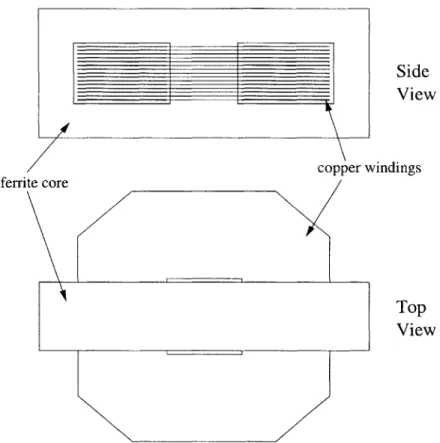
The magnetic structure of the transformer consists of a ferrite E-core with the windings surrounding the center post, as shown in Figure 1-3. The windings are made

Figure 1-1: DC to DC converter Primary Iturn ... x6... i turn ... x 6... I turn _{... x6 ...} I turn ... x6.. Secondary 12 turns 12 turns

Figure 1-2: Connections to primary and secondary windings V+

0-V.

Side View copper windings ferrite core Top View

Figure 1-3: Magnetic structure of transformer

of flat copper sheets separated by thin layers of insulating material. The structure of the windings is designed to increase the current density handling capability that is required during normal operation at high frequencies. This is due to the fact that the flat-winding construction of the transformer has several advantages over conventional windings for carrying high current density at a high frequency. Copper sheets with thin layers of insulation between them allow for a much higher packing factor than conventional windings made of rounded insulated wire, as the fill factor is higher for the flat sheets. The resulting effective area of the windings is higher, allowing the windings to carry greater current density. The shape of the windings also has the effect of giving the transformer better performance at high frequency. The thickness of the windings is less than the skin depth of the copper at 30 kHz, so the skin effect is reduced at high frequencies as well as the proximity effect.

However, the use of flat copper conductors in the windings raises other design issues. The flat windings running parallel to each other behave as parallel plate

ca-pacitors, causing inter- and intra-winding capacitances to become significant. The primary and secondary windings are interleaved in order to reduce the leakage induc-tance of the transformer. However, interleaving the windings greatly increases the parasitic capacitance between the primary and secondary windings, resulting in un-planned resonant frequencies affecting the behavior of the transformer. Capacitance was therefore one of the more important transformer characteristics considered by this thesis.

An attempt was made to analyze the transformer using three-dimensional finite element analysis. However, the geometry of the transformer did not lend itself well to construction of the finite element analysis mesh. Each of the flat windings is about three inches in length and width but only 0.016 inches in thickness. The large difference between the largest and smallest dimension means that a very fine mesh is needed over a large surface area in order to accurately analyze the model. The amount of memory needed to run the simulation exceeded that found in the average computer. The difficulty of performing a physical analysis of the transformer behavior demonstrated the need for a simpler way to accurately predict transformer behavior.

1.2

Technical approach

Preliminary tests of the power conditioning circuit indicated that the transformer was overheating under normal operating conditions. The transformer needed to be made more efficient in order to function effectively as a power transfer device. The objective of this thesis was to allow the transformer and its surrounding circuitry to be improved for efficiency based on a complete description of its behavior.

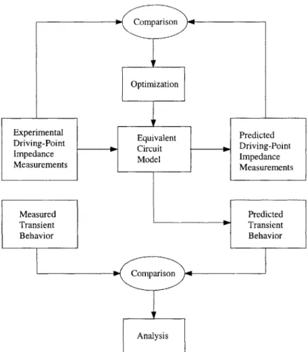
The procedure for characterizing and optimizing the model is outlined in Fig-ure 1-4. Extensive experimental impedance measFig-urements were carried out, leading to the initial calculation of parameter values for an equivalent circuit model of the transformer. The parameter values were then modified by an optimization procedure to minimize the difference between the equivalent circuit behavior and experimental data points. Simulations were run on the equivalent circuit model in order to

rep-Optimization

Experimental Equivalent Predicted

Driving-Point qCircuit Driving-Point

Impedance Model Impedance

Measurements _Measurements

Measured Predicted

Transient Transient

Behavior Behavior

AnalysisI

Figure 1-4: Block diagram of procedure

resent the behavior of the transformer in its operating environment. The modeling technique was analyzed for its ability to predict the impedance characteristics of the transformer and its performance in its operating environment.

The procedure for carrying out impedance measurements on the transformer is described in Chapter 3. Open circuit and short circuit driving-point impedance mea-surements were recorded for various measurement configurations.

The impedance measurements were used to identify parameters for an equivalent circuit representation of the transformer. Chapter 4 describes how the inductance, resistance, and capacitance values were calculated based on the measurements. The equivalent model was optimized for close correspondence between the simulated and measured impedances using error minimization techniques.

model. Chapter 5 describes the circuit simulation software and the equivalent circuit model. The transformer was simulated both as a stand-alone unit and with inputs that simulate its operating environment. The simulations were compared to the various measurement results as well as actual waveforms recorded from tests on the power electronics unit.

The performance of the model was checked against data taken from testing the transformer, and the effectiveness of the equivalent circuit to predict the transformer properties was analyzed. The results of this analysis are described in Chapter 6.

Chapter 2

Previous Work

Many different approaches have been taken to modeling transformers. Developing an equivalent circuit model for a given transformer is a particularly important task, as it allows the circuit containing the transformer to be simulated and tested for per-formance before circuit construction. Some of the methods involve using the physi-cal characteristics of a transformer to explain its behavior, while others attempt to describe the transformer using equivalent circuit parameters not dependent on the physical transformer.

Extensive work in this field has been done by the magnetics group at the Labora-toire d'Electrotechnique de Grenoble, France. An experimental method for producing an equivalent circuit model for a transformer is presented in [4]. The method relies only on external open-circuit and short-circuit driving-point impedance measurements taken at the primary and secondary of the transformer. The equivalent circuit in-cludes terms for parallel and series inductance, losses, and parasitic capacitances. The advantage of the model is that it is valid for a wide range of frequencies but is independent of the geometry and construction of the transformer. Transformers of different shape or technology can be represented by the same model with different circuit parameters.

Calculation of capacitances in the equivalent circuit is treated more thoroughly in [1]. The total electrostatic energy stored in a two-winding transformer is shown to depend on six coefficients and three independent voltages. Therefore, the capacitive

effects seen from the terminals of the transformer can be completely described by six capacitors, appropriately placed in the circuit. The six values can be obtained using different measurement configurations in which certain terminals of the transformer are electrically connected. The model then simplifies to a partial equivalent circuit with three capacitor values. An expression for the energy stored by the capacitors is obtained in each case, and this can be used to calculate the six capacitance values of the total equivalent circuit. The capacitor values for the partial equivalent circuits can be found using resonance frequencies, once the open-circuit and short-circuit in-ductance values of transformer are known. Similarly, once the capacitor values are known, the resonant frequencies can be predicted. The paper also presents a micro-scopic approach to calculating capacitances and general rules for reducing capacitance in windings.

The equivalent circuit representation of transformers is also given extensive treat-ment in [3]. Each component of the lumped-parameter equivalent circuit model is discussed, including elements for magnetic coupling; winding resistance, core losses, and eddy current losses; and capacitance between the windings. Calculation of the component values for a two-winding transformer is demonstrated through an exam-ple, and a comparison of experimental and theoretical results is presented. The paper also discusses measurement techniques and configurations and issues of accuracy that may arise from impedance measuring equipment.

Transformers of more than two windings are described in [7], which presents a different method for calculating equivalent circuits, related to the method described

by the previous work in [4], [1], and [3]. The method allows for transformers with an

arbitrary number of windings to be modeled. It also accounts for situations where certain resonant frequencies, which are needed to calculate component values, are out of the range of the measuring apparatus. Rough equivalent circuit models of the transformer are refined in successive steps to make a more and more accurate model. Multiwinding transformers have also been treated in [6], [8], and [2]. [6] uses

a network of circuit elements to model the frequency dependence of resistance and inductance values in the equivalent circuit. This allows the ac winding resistanee and

leakage inductance to be calculated over a range of frequencies for high-frequency transformers with any number of windings. A physically-based approach to modeling a multiwinding transformer is given in [8]. The method described was used to more accurately predict leakage inductances in high-voltage multiwinding transformers. The transformers described in the paper all have coaxial windings, however. Leakage inductances are also the focus of [2], which uses the finite element method to relate each parameter of the model to a specific flux in the physical transformer. The form of the model, however, does not depend on the physical geometry of the transformer. Modeling of a magnetic system with a complicated geometry was performed in [5]. The paper develops a lumped-parameter model to calculate the voltage distribution in a helical armature winding. The model uses electrical cells to represent the windings, including self and mutual inductance between the cells, capacitance between the cells, and capacitance to ground. The values of the parameters are calculated based on the physical structure of the system.

The previous work serves as a basis for this thesis. The method described in [4],

[1], and [3] is used here to develop an equivalent circuit model for the transformer.

The method had not been previously applied to a transformer with flat windings, and thus it was of interest to determine if the methods extend to this particular topology. Capacitance values were expected to play a particularly large role in the behavior of the transformer, while other factors such as eddy current losses were expected to have a much smaller effect. The equivalent circuit model was simplified in order to focus on the effects which were expected to dominate the transformer's behavior.

Chapter 3

Methods

A circuit model of the transformer was selected, and the values of the circuit

compo-nents were identified through experimental measurements on the transformer. The equivalent circuit chosen to model the transformer was the one described by Cogitore

[3]. A set of measurements was taken at the various transformer terminals in

or-der to determine the parameters representing transformer behavior. The parameters to be determined included magnetic constants, losses, and electrostatic constants. These constants were determined through open-circuit and short-circuit impedance measurements at the various terminals.

3.1

Equivalent circuit model

The equivalent circuit model used for the analysis is shown in Figure 3-1 and includes all the components to be identified. Each circuit element represents a different phys-ical phenomenon affecting the behavior of the transformer. Lp represents the parallel inductance of the transformer, while L, represents the series inductance. The resistor R, represents core loss, and DC winding resitances are accounted for in r, and r2.

Eddy current and proximity effects are neglected in this circuit as a simplification,

since the expected eddy current losses are low due to the winding structure. The six capacitors in the circuit represent all possible capacitive couplings observed at the terminals of the transformer [1].

C5 C4 C6 rl Ls r2 A 1Ns - C Secondary Cl 2Rp 2Lp 2Lp 2Rp C2P B 4 C3

Figure 3-1: Equivalent circuit model of transformer

A + + C

V

V

Figure 3-2: Three independent voltages of a two-winding transformer

A two-winding transformer has at most three independent voltages, depicted in

Figure 3-2: the voltage on the primary, the voltage on the secondary, and the voltage difference between one terminal of the primary and one terminal of the secondary. The stored electrostatic energy of the system is a function of the three voltages:

WE 1 2 - 3 3 2+V C1 2V1V2 + C1 3V1V3 + C2 3V2V3 (3.1)

2 2 2

The six coefficients C1 - C2 3 completely characterize the electrostatic behavior of the

transformer. [1]

A o-C1 --B 0-C5 C4 inductive and resistive components C6 ideal coupling I C2 C3

Figure 3-3: Six capacitors of the equivalent circuit model

equivalent circuit model. The stored electrostatic energy in this circuit is given by 1 WE =-2 V2 + 1 C2 ( ± 1 C 1 2 N 2 CV3+4 V2 2 + I 1 1 72 (

7_)

Equating the expressions of Equations 3.1 and 3.2 gives expressions for the six capac-itors of the equivalent circuit model in terms of the coefficients Cu - C_{2 3}. [3]

C1 = C11 + NC12 + C1 3 C2 = N2C2 2 + NC12 + NC2 3 C3 = C33 + C13 + NC23 C4 = -NC 12 C5 = -C13 C6 = -NC 23 -0 _C D

Configuration Experiment Shorted Driving point connections impedance port

BD 1 BD AB 2 BD,CD AB 3 BD CD AB CD 4 AB,CD BD AC 5 AC AB 6 AC,CD AB BC 7 BC AB 8 BC,CD AB AD 9 AD AB 10 AD,CD AB Table 3.1: Experimental measurements

3.2

Experimental measurements

Identification of the equivalent circuit parameters involved the use of driving point impedance measurements. Different conditions of the impedance measurements were used to compute the various circuit elements. Low frequency values of the inductance, resonant frequencies, and peak impedance values were observed from the measure-ments and used to calculate the parameter values.

There were four possible models that could be developed for the transformer under study, depending on whether the center tap was used as a connection. The measurements could utilize half or all of the primary or secondary winding. The model using the full secondary winding and half of the primary winding was chosen for its significance in later simulations, using the secondary as port AB and half of the primary as port CD. For completeness and to verify the accuracy of the modeling method, measurements were recorded for the three other transformer models. A description of those measurements can be found in Appendix C.

Several sets of driving point impedance measurements were taken at the terminals of the transformer. The various experiments are listed in Table 3.1.

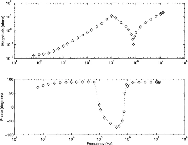
10 10 102 103 0 105 10 10 10" 10 0-) 0 -100 50 1 ci) 0) 0 -100 12310 10 10 10 10 10 10 10678 Frequency (Hz)

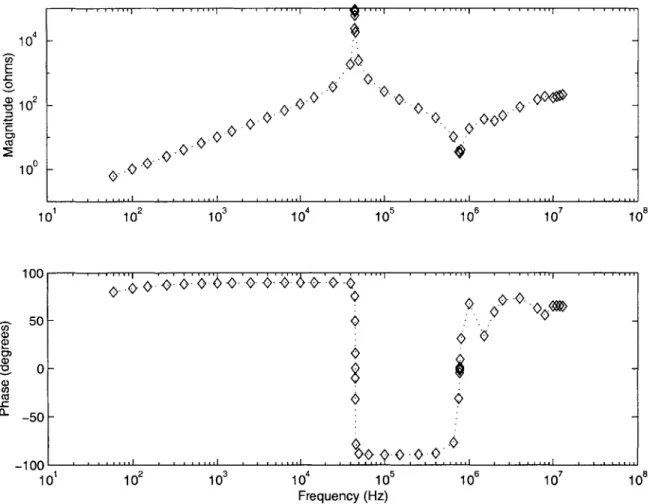
Figure 3-4: Impedance of secondary, primary open

3.2.1

Configuration BD

Three full plots of the driving point impedance were made for the configuration in which B was connected to D. The first plot measured the impedance seen from the secondary (AB) with the primary (CD) open, the second the impedance seen from AB with CD shorted, and the third the impedance seen from CD with AB open. The magnitude and phase of the impedance were recorded over a range of frequencies from 60 Hz to 13 MHz. Plots of the measured impedance are found in Figures 3-4,

3-5, and 3-6.

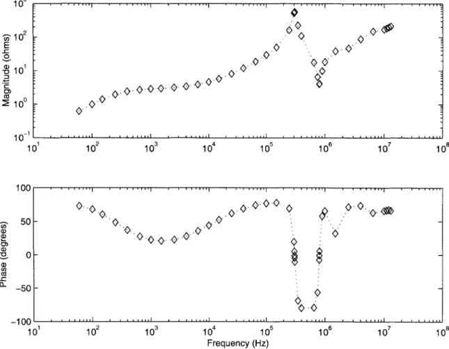
The experiments performed with configuration BD allowed for the calculation of the inductive and resistive parameters in the equivalent circuit model and provided information relevent to the calculation of the capacitor values, as described in

Chap- 0--'0' 0 0 --0 101-1 0-01 10 102 105 Frequency (Hz) 10 10 7

Figure 3-5: Impedance of secondary, primary shorted

10 E -0 70 1 C W 10 10 10 10 5 -5 C,, a) U, U) V a, C,, CU -c 0~ ~10A 10 )8 10 3 10

C

1 2 3 4 5 6 7 10 10 10 10 10 10 10 1C )

0

-

Figure 3-6: Impedance of primary, secondary open - 10 E 0 CD) 0 v 10 C 10-10 10 0), CD 0) CU CL ~10f 10 102 8 0 5 --5 10 4 10 7 10 8

ter 4.

The measurements using this configuration were later compared to bode plots of the impedance of the equivalent circuit model in order to verify the accuracy of the model.

3.2.2

Configuration AB CD

When the ports AB and CD are shorted, V1 = 0 and V2 = 0. Equation 3.1 reduces to

WE C 3 3 32 (33)

2

Measuring the capacitance between terminals B and D gave the capacitive coefficient

C33. The measurement was taken at several low frequencies in order to confirm the

accuracy of the measurement.

C3 3 = 12.8nF

3.2.3

Configurations AC, BC, and AD

Open-circuit and short-circuit driving point impedance measurements were taken for each of the remaining configurations in Experiments 5 through 10. In each case the impedance was measured from the transformer secondary, AB, while the primary,

CD, was either open or shorted. The first two resonant frequencies were recorded

for each open-circuit experiment, and the first resonant frequency was recorded for each short-circuit experiment. The point where the phase of the impedance crossed zero was observed and used to precisely determine the resonant frequency. Capacitor values for the equivalent circuit model depend on the resonant frequencies of the various measurement configurations.

The measured frequencies are listed in Table 3.2. The resonant frequencies of configuration BD are also listed.

fp

f,

Configuration fp,open fs,open fp,short

BD 45.43kHz 773kHz 307kHz

AC 41.96kHz 723kHz 317kHz

BC 51.05kHz 850kHz 330kHz

AD 48.72kHz 814kHz 337kHz

Table 3.2: Experimental measurements

The ten experiments gave enough data to overdetermine the eleven equivalent circuit parameters. With more than the necessary amount of data, redundant results could be compared against each other for consistency.

3.2.4

Equipment

The relatively low impedance of the transformer made impedance measurements dif-ficult. Preliminary impedance characteristics were measured using a Hewlett-Packard

4395A network analyzer. The frequency characteristics measured by the network

an-alyzer showed significant differences from measurements taken using a current probe and oscilloscope. High frequency resonances occurred at different frequencies and the shape of the waveform differed slightly at low frequencies. It was speculated that impedances internal to the network analyzer and its probe were changing with fre-quency in a way that could not be measured or compensated. These speculations were supported by similar problems related in [3]. Since the test configuration for using the HP4395A as an impedance analyzer was not available, measurements were instead carried out on a Hewlett-Packard 4192A impedance analyzer. The impedance analyzer can measure low impedances with greater accuracy than a network analyzer. The method of [3] required that various driving-point impedance measurements be taken over a swept range of frequencies. Two impedance measurements were to be taken from side AB of the transformer (one with the leads CD open and one with the leads CD shorted together) and one impedance measurement was to be taken from side CD (with the port AB open). The equivalent circuit parameters depended more heavily on the measurements taken from side AB than on those taken from

the side CD. The accuracy of the model may depend on the choice of which side of the transformer is considered as AB and which is CD. Since measurements of lower impedances run a greater risk of error due to equipment inaccuracies, more accurate results are likely to be obtained when the side chosen as port AB has a higher impedance. It was expected that more accurate results would be obtained by choosing the side of the transformer with the greater number of turns to represent AB, since a greater number of turns made the impedance seen from this side of the transformer slightly higher.

The secondary side of the transformer in question was chosen to correspond to the port AB. The secondary of the transformer had a higher number of turns and therefore the expected impedance was higher.

The HP4395A did not have automatic sweep measurement or data recording ca-pability in the configuration that was available to perform the testing. Individual data points had to be read and recorded manually. As a result, measurements are discrete rather than continuous, and the data is not as thorough as the measurements recorded in [3].

Chapter 4

Identification of the Equivalent

Circuit Parameters

The values of the circuit components were calculated using external impedance measurements. The experimental method described in [3] for creating a lumped-parameter equivalent circuit depends on the open-circuit impedance measured from both sides of the transformer and the short-circuit impedance measured from one side. Different aspects of the impedance measurements, taken as a function of frequency, were used to compute the various circuit elements. Low frequency values of the inductance, resonant frequencies, peak impedance values, and mid-frequency impedance values were observed from the measurements and used to calculate the parameter values.

Figure 4-1 shows a simplified version of Figure 3-1, using the configuration in which terminal B is connected to D. If this connection is made, the capacitor C3

is eliminated from the circuit, the capacitor C5 is in parallel with C1, and C is

in parallel with C2. The resulting circuit can thus be described by three capacitor

values, as shown in Figure 4-1, where CA is equal to C1 + C5, CB is equal to C2 + C6,

and Cc is equal to C4. This simplified circuit was used to calculate the resistive

and inductive circuit components of the model and to compare predicted impedance with the measurements described in Chapter 3. Measurements using the remaining configurations were later used to define all six capacitor values shown in Figure 3-1.

Cc ri Ls r2 A NS Secondary CA 2Rp 2Lp 2Lp 2Rp CB Primary SD B T

Figure 4-1: Simplified equivalent circuit model of the transformer

4.1

Modification of the equivalent circuit

The measured open circuit and short circuit impedance curves differed from those predicted by the equivalent circuit model in [3]. In particular, there was an additional series resonance in the short circuit impedance that was not found in [3], and a positive slope to the high frequency impedance in both the open and short circuit case, shown in Figures 3-4 and 3-5. These characteristics suggest that an additional inductive element was present in the measured impedance that was not accounted for in the equivalent circuit. A filter present on the measurement equipment was suspected to have caused the additional inductance.

Figure 4-2 shows a modified version of Figure 4-1. The circuit does not contain any resistive elements and has an additional inductor Lx representing the inductance of the measurement setup. In addition, to simplify the consideration of the driving point impedacne seen from port AB with port CD open, the ideal coupling and the port CD are not included. Figure 4-3 shows the circuit of Figure 4-1, simplified for the case in which port CD is shorted and the driving point impedance seen from port AB is considered.

The parameters Lx, L,, and L, were estimated based on the impedance mea-surements and the circuits of Figures 4-2 and 4-3, as discussed below. The resonant frequencies of the measured impedance were used to refine the estimates of the in-ductances and calculate the values of the capacitors CA, CB, and Cc. Finally, initial estimates of the resistive parameters were refined in order to fit the measured data. The calculated values can be found in Table 4.1.

Lx

A

Secondary

Figure 4-2: Simplified circuit with additional inductance

Lx

A rJ~ Y ,

Secondary

CA+CC _{2Lp Ls}

Figure 4-3: Simplified circuit with additional inductance

using the value of the measured high frequency impedance. Expressions for the low frequency open circuit inductance, LO, and the low frequency short circuit inductance, LC, were derived using the equivalent circuits of Figures 4-2 and 4-3.

LO = L, + 2LI|(2Ls + 2JL,) _(4.1)

(4.2) Based on the circuit of Figure 4-3, an expression for the frequency of the parallel resonance can be found.

Wp,short

1

(CA + Cc)(Lc - Lx)

The short circuit series resonance is given by

Ws,short = (4-3) (4.4) 1 (L(1 - 77-j (GA + GO Lc = Lx + 2LpIILs

A script written in Matlab iteratively determined the values of L2, L,, L., and

CA + CC which fit the measured low frequency inductance and short circuit resonant

frequencies. The script is included in Appendix B.

The resonant frequencies of the open circuit model were used to determine the three capacitor values, given the constraint on the value of CA + Cc. The open circuit

equivalent model of Figure 4-2 has four resonant frequencies: two series resonances, or peaks in the impedance graph, and two parallel resonances, or troughs in the impedance graph. In Figure 3-4, for example, the first series and parallel resonant frequencies are easy to observe. The second two resonant frequencies occur close together and are more difficult to observe. The phase plot of the impedance is helpful in estimating the higher resonant frequencies.

Due to the complex nature of the expression for the impedance of Figure 4-2, a mathematical program was used to derive the expression, which can be found in Appendix A. A Matlab script determined the values for the capacitors CA, CB, and

Cc which matched the measured resonant frequencies to the roots of the numerator

and denominator of the impedance expression. The script is included in Appendix B. The calculated values can be found in Table 4.1.

4.1.1 Coupling coefficient

The coupling coefficient for the equivalent circuit is calculated from the low frequency open-circuit inductance seen from the secondary of the transformer and that seen from the primary. The coefficient for the ideal coupling is given by

Ns = LoP (4.5)

Los

where Los and Lop are the low frequency open-circuit inductance seen from the secondary and primary, respectively. The low frequency inductance of the secondary (port AB) is just Lo - L, from Equation 4.1. Similarly, the low frequency induc-tance of the primary (port CD) can be calculated from the measured low frequency inductance of Experiment 3 (Table 3.1) by subtracting L,. The calculated coupling

coefficient, Ns = /1=16x10 5 _{0.0854, closely approximates the known turns ratio of}

the transformer, 2 = 0.0833.

4.1.2

Loss parameters

The value of the parallel resistance Rp was determined by calculating the height of the first resonant peak in the open-circuit impedance measured from the secondary, shown in Figure 3-4. This resistance represents core losses in the transformer.

There are several possible ways of determining the DC winding resistance for each winding. One way is to note that the resistance plotted versus frequency for the open-circuit impedance of the secondary at low frequencies gives rl, the DC winding resistance of the secondary. The low frequency resistance calculated from the open-circuit impedance measured from the primary gives Njr2, the DC winding

resistance seen from the primary. This method of calculation gave r, = 5.5Q and

r2 = 2.4Q. As a check, the short-circuit impedance of the secondary at low frequencies

can be used to determine r1 + r2, the total DC winding resistance seen from the

secondary. However, the value for r1 +r 2 was calculated to be 1.5Q. The two methods gave inconsistent results. Measurement noise and error can account for the difficulty in calculating these two values. An ohmmeter capable of determining very small resistances was used to measure the values of the low frequency resistance seen from both the primary and secondary. Even with this piece of equipment, there was a great deal of measurement noise, and the values for r1 and r2 are only close approximations.

However, since the ohmeter was the most direct method of measuring r1 and r2, the resistance measurements were used for the initial estimates of r, and r2.

Since the resistor values Rp, rl, and r2 of Figure 4-1 had only been estimated previously, a Matlab script was run which selected values for the resistor parame-ters. The script attempted to minimize the difference between the predicted circuit impedance and the measured points over the entire range of frequencies. The resistor values can be found in Table 4.1.

4.2

Optimization procedure

Since the impedance of the equivalent circuit is a complicated mathematical expres-sion depending on all the circuit parameters, Matlab was used as a mathematical aid in optimizing the equivalent circuit. Scripts written in Matlab adjusted the cir-cuit parameters to make the predicted impedance more closely match the measured impedance. The scripts would often minimize the error between the impedance of the equivalent circuit and the measured impedance data points. Initial estimates for the parameters were given to the programs as a starting point, and the script was allowed to change one or more component values in order to find a local minimum for the error.

Several attempts were made to optimize the equivalent circuit by varying all circuit parameters simultaneously. The program was given an initial set of parameter values and was able to vary those parameters until it found a minimum for the difference between the predicted and measured impedance. Since the function to be minimized was often complicated and nonlinear, the results depended heavily on the initial values given. The exact definition of the error function also played a significant role in determining the final results. For example, data points in certain frequency ranges could be weighted more heavily than others, or the program could consider the absolute or relative error of the values. The varying nature of the program output indicated a strong need for a more intelligent optimization process.

As described in Section 4.1, the values of the inductances could be determined with confidence from the measured data points. The capacitances could then be determined as well. Once those parameters were set, it was easier to determine the remaining resistor values.

Equations 4.1 through 4.4 allowed for the calculation of the inductors in the circuit, as well as the sum of the capacitor values CA + Cc. Given the measured values of the low frequency inductances Lo and L, and the resonant frequency wp,short, the program used an estimated value of L. to determine the remaining inductances and the value of CA + Cc. L, was then recalculated using the value for Ws,short and an

iterative process continued until the value for L, no longer changed.

With the inductive values already determined, the program used the four open circuit resonant frequencies to calculate CA, CB, and Cc. The constraint on the value of CA+ Cc gave two degrees of freedom to determine the three capacitor values. A

minimization script was used in this case. The function minimized the difference be-tween the predicted and measured resonant frequencies, weighting all four resonances equally.

The three resistive parameters were determined using another minimization script. The function minimized the difference between the predicted and measured impedance in both the open and short circuit case, calculating the error over a range of data points. Since more data points were taken around the resonant frequencies of the impedance, some points around the resonant frequencies were eliminated from the minimization script. This prevented the program from giving too much weight to the value of the function near the resonant frequencies. The program took the measured

Rp, r1, and r2 as initial values. The error value was increased whenever the resistor

values differed from their original values by more than 15 percent, thereby ensuring that the calculated values were still realistic.

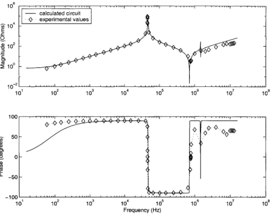
Final circuit parameter values are shown in Table 4.1. It should be noted that the negative value for Cc does not pose a problem, since only capacitances which can be measured physically are required to be positive. Figures 4-4 and 4-5 show the predicted driving-point impedance of the equivalent circuit model, using the param-eter values of Table 4.1. The predicted impedance is plotted with the measured data points from Figures 3-4 and 3-5.

The operating frequency of the transformer is 30 kHz. However, since the driving waveform will be a square wave with varying duty cycle, frequencies higher than 30 kHz are relevant to the operation of the transformer. Frequencies below 30 kHz may also be important as the duty cycle varies with time. The optimized circuit values match the measured impedance in a frequency range several orders of magnitude above and below the operating frequency. The optimization also yields circuit pa-rameter values that are very close to the original calculated values. The result of the

10 1 102 103 104 10 10 10 Frequency (Hz) - calculated circuit 10 - experimental values 1 2 -0 10 -10-2 10 102 103 104 105 10 10 10 100 50-0 -50-.100 108

Figure 4-4: Open circuit impedance, measured and predicted

102 10 0 10 0 --50 10 2" 102 103 104 105 10 10 10 10 102 103 104 Frequency (f 105 10 10 10

Figure 4-5: Short circuit impedance, measured and predicted

E -c_ 0 0) Ca C .) IL 104 calculated circuit - experimental values - -0 E -c 0 C cc CO 10~2 10 1 U) 0o CL 6 8

-L, 6.81pH LP 1.57mH L, 40.5pH Rp 78.OkQ r1 685mQ r2 32.3mQ CA 6.81nF CB 0.41nF Cc -0.088nF Ns 0.0854

Table 4.1: Optimized circuit parameter values

optimization affirms the accuracy of the model within a wide frequency range. There were certain tradeoffs in the optimization procedure. The new impedance curve no longer matches the magnitude of the resonant peaks as closely as it did before. However, it was considered most important to match the frequency values of the resonance and the high and low frequency inductor values.

4.3

Calculation of six capacitor values

The majority of the measurements on the transformer were taken with the config-uration shown in Figure 4-1, where B on the secondary was connected to D on the primary. However, in order to calculate all six capacitor values in Figure 3-1, resonant frequencies are needed from other measurement configurations.

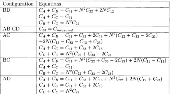
The first series and parallel resonant frequencies for the open and short circuit impedance was recorded for all measurement configurations described in Chapter 3 and listed in Table 3.1. The three capacitor values CA, CB, and Cc were determined for each case. Table 4.2 shows how the capacitor values for each measurement config-uration relate to the capacitive coefficients of Equation 3.1, as described in [1]. The measurements generated thirteen equations with which to calculate the six unknown capacitances. The capacitors values are overspecified by the available information.

ca-Configuration Equations BD CA + CB= C11 + N2C2 2 + 2NC12 CA +CC =C11 CB + Cc =N 2 C22 AB CD C33 = Cmeasured AC CA + CB Cn + C33 +2C 13 +

N

Table 4.2: Equations relating capacitance values for various measurement configura-tions

BD AC BD BC BD AD BC AD Best fit CC fit CAandCB fit C1 124.9nF -405.8nF 110.6nF 99.2nF 163.9nF 162.2nF 107.5nF C2 6.31nF -39.6nF 4.91nF 150.1nF 24.5nF 25.7nF 40.OnF C3 15.3nF -30.7nF 26.lnF 306.4nF 52.5nF 54.7nF 52.4nF C4 -3.52nF -3.52nF -3.52nF 119.2nF -3.9OnF -.088nF -.088nF C5 -114.7nF 527.5nF -100.3nF 11.11nF -44.2nF -42.5nF -100.7nF C6 -2.47nF 43.5nF -13.3nF -293.5nF -39.7nF -41.9nF -39.6nF

Table 4.3: Values for six capacitors

pacitor values, the capacitors were calculated many different ways and the results were compared against each other. All calculations utilized the measurement from configuration AB CD, which gave the value for C33. The first calculation combined data from when B and D from Figure 3-1 are connected together (configuration BD) and from when terminals A and C are connected together (configuration AC). The second calculation used configuration BD and configuration BC, the third configura-tions BD and AD, and the fourth configuraconfigura-tions BC and AD. The resulting values are shown in Table 4.3.

It should be noted that, although a capacitance which can be directly measured can only be positive, the capacitors of the equivalent circuit are not necessarily directly related to meaurable capacitances in the transformer. The six capacitors in total represent the electrostatic interactions in the transformer, and since some couplings may reduce the stored electrostatic energy, the capacitances are allowed to be negative

[1].

Considering the wide variety of resultant capacitor values, it was deemed appro-priate to calculate a best fit for the unknown capacitances. A set of twelve equations for the five remaining unknowns was processed by Matlab, giving equal confidence to all equations. The results appear in Table 4.3 in the column labeled "Best fit".

Since the configuration of Figure 4-1 was more completely characterized than the other measurement configurations, there is more confidence in the capacitor values calculated from that configuration. Cc in Figure 4-1 is the same as C4 in Figure 3-1, eliminating one of the unknowns from the set of equations. Taking this into account yields the results in column "Cc fit". Finally, C1

+

Figure 4-1, and C2 + 06 in Figure 3-1 is equal to CB in Figure 4-1. The values for CA and CB, as well as that for Cc, were matched by the final calculation. The results are in column "CA and CB fit".

The difficulty in finding a consistent set of capacitor values plays a significant role in the effectiveness of the equivalent circuit under simulation.

Chapter 5

Simulation

The measurements and calculations of the previous chapter were used to develop the circuit diagram shown in Figure 5-1 as described in [3]. Figure 5-1 is identical to Fig-ure 3-1, but the values for the inductances, resistances, and coupling coefficient have been included in the figure. L represents the parallel inductance of the transformer, while L, represents the series inductance. The resistor Rp represents core loss, and

DC winding resitances are accounted for in r1 and r2. The six capacitors in the circuit

represent all possible capacitive couplings between the terminals. The ideal coupling of the equivalent circuit was represented in simulation by a voltage-controlled voltage source and a current-controlled current source of identical gain.

5.1

Simulation tool

Simulations of the equivalent circuit were performed using Simplorer circuit simu-lation software. Simplorer allows a circuit schematic to be entered with values for each of the components. An equivalent circuit can be driven by a sinusoidal source over a range of frequencies, or by a source of arbitrary waveform. Both types of analysis were used in this case, since both frequency-dependent characteristics and time-domain transient performance were important to the model. Simplorer can cal-culate and plot various voltages and currents for a given input. Simplorer will also calculate mathematical combinations of voltages and currents that allow calculation

C5 C4 C6 T1 Ls r2 Ns A 0.0854:1 C 685 m 40.5 uH 32.3 m Secondary Ci 2Rp 2Lp 2Lp 2Rp C2Pr 156k 3.14 mH 3.1D4 mH B o C3

Figure 5-1: Circuit model of transformer

of other important considerations, such as magnitude and phase.

As described in Section 4.3, the capacitors in the equivalent circuit may take on negative values, provided that no capacitances which can be measured directly are negative. Simplorer accepts negative values for capacitors without giving an error. Simplorer will, however, give unstable results in transient simulation if the combination of capacitor values results in a physically impossible situation, one in which measurable capacitances in the circuit would turn out to be negative. This fact provides an additional check for the appropriateness of the capacitor values in transient simulation.

5.2

The transformer as a stand-alone circuit

In order to confirm the ability of the model to represent the transformer as it was experimentally measured, the transformer was simulated as a stand-alone circuit. AC sweep analysis was performed in order to find the voltage to current ratio seen from the secondary side of the transformer. A resistor of value 1 Megaohm placed across the primary of the transformer simulated an open circuit, while a resistor of 1 milliohm placed at that winding simulated a short circuit. The open-circuit and short-circuit impedances from the simulation were compared against the experimentally measured

102 103 104 105 10 10 108

2 3 4 5

102 10 104 10

Frequency (Hz)

10 10 10

Figure 5-2: Open circuit simulation, configuration BD values.

The measurement configuration of Figure 4-1, configuration BD, was used for the first set of simulations. Therefore, the capacitor values CA - Cc were used, rather than C, - C6. The component L; was included in the circuit so that it could be

compared accurately to the measured data.

The simulated data is plotted with the measured data points in Figures 5-2 and

5-3. The plot closely matches the measured impedance, as predicted by the previous

analysis and summarized in Figures 4-4 and 4-5.

Since the actual circuit under operation does not have terminal B connected to terminal D, it is important to consider the accuracy of the six capacitor circuit of Figure 3-1. The driving point impedance of the secondary (AB) of the six capacitor circuit was simulated and compared against a set of measurements in which no con-nection had been made between the secondary and primary. Since there were many possibilities for the six capacitances, the simulation was performed for each case in

me --- sin 106 2 10 E -C 10 10) 2 100 102 L 10 CI) a) cc 0) ~0 100 5 0- -50--100 10 ~

L

measured - simulated E 102 10 10 10 12 3 4 5 8 10 10 10 10 10 10 10 10 (n 50-0 - -50-101 102 103 104 105 10 10 108 Frequency (Hz)

Figure 5-3: Short circuit simulation, configuration BD

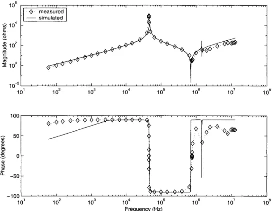
Table 4.3. The simulation results for all cases are plotted together in Figure 5-4. The resonant frequencies of the open circuit impedance do not resemble the mea-sured values, no matter which set of capacitor values is used. The inconsistency of the six capacitor values calculated from various measurements on the transformer implied a lack of confidence in any of the capacitor values. The plot of the simulated impedance shows that the choice of capacitor values has a significant effect on the equivalent circuit behavior. Despite the close correspondence obtained for the case in which only three capacitors are significant, the equivalent circuit does not accurately

predict transformer behavior for all measurement configurations.

A closer fit was obtained by arbitrarily changing capacitor values to alter the

resonant frequencies. For example, it was noted that the resonant frequencies of the simulated impedance were lower than those of the measured impedance for all cases in Figure 5-4. An effort was made to increase the resonant frequency values by changing the capacitor values. Simulated impedance using the values in Table 5.1 is shown in

-3 3 3 -N T T W .I