Can we trust the inter-packet time for traffic classification?

HAL Id: inria-00546794

https://hal.inria.fr/inria-00546794

Submitted on 21 Jan 2011

HAL is a multi-disciplinary open access

archive for the deposit and dissemination of

sci-entific research documents, whether they are

pub-lished or not. The documents may come from

teaching and research institutions in France or

abroad, or from public or private research centers.

L’archive ouverte pluridisciplinaire HAL, est

destinée au dépôt et à la diffusion de documents

scientifiques de niveau recherche, publiés ou non,

émanant des établissements d’enseignement et de

recherche français ou étrangers, des laboratoires

publics ou privés.

Can we trust the inter-packet time for traffic

classification?

Mohamad Jaber, Roberto Cascella, Chadi Barakat

To cite this version:

Mohamad Jaber, Roberto Cascella, Chadi Barakat. Can we trust the inter-packet time for traffic

classification?. [Research Report] 2011. �inria-00546794�

Can we trust the inter-packet time for traffic

classification?

Mohamad Jaber, Roberto G. Cascella and Chadi Barakat

2004, Route des Luciolles Sophia Antipolis, France

Email:{mjaber, rcascell, cbarakat}@inria.fr

Abstract—The identification of Internet applications is impor-tant for ISPs and network administrators to protect the network from unwanted traffic and prioritize some major applications. Statistical methods are widely used since they allow to classify applications according to their statistical signatures. They com-bine the statistical analysis of flow parameters, such as packet size and inter-packet time, with machine learning techniques. Previous works are mainly based on the packet size and the directions of the packets.

In this work we make a complete study about the inter-packet time to prove that it is also a valuable information for the classification of Internet traffic. We discuss how to isolate the noise due to the network conditions and extract the time generated by the application. We present a model to preprocess the inter-packet time and use the result as input to the learning process. We discuss an iterative approach for the on line identification of the applications and we evaluate our method on two different real traces. The results show that the inter-packet time is an important parameter to classify Internet traffic.

I. INTRODUCTION

Internet Service Providers (ISPs) and network administra-tors are more and more interested in identifying the appli-cations behind Internet traffic to protect the network from unwanted traffic and to prioritize some major applications. The recognition of applications should help to take the right decision for the control of the quality of service and for the dimensioning of the network.

The recognition of applications in IP traces becomes in-creasingly complex. Historically, this recognition was based on static and standard port numbers in the transport header, but the use of dynamic port numbers or of standard ports to hide other applications causes this solution to be ineffective. Current techniques of “Deep Packet Inspection” (DPI) [1] make it possible to go further in the identification of the applications but they require a complete and costly exploration of the payload of the packets. This induces an important load and is not practical when packets are encrypted.

Statistical techniques [2]–[8] seem to be today a promising alternative. They allow to recognize and to classify the applica-tions according to their statistical signatures. These signatures can be data volume (e.g., number of bytes) per connection, connection duration, rate, inter-packet delay, packet size, and direction. Most of the papers in the literature rely on the packet size to identify the applications.

Several papers [5]–[8] discuss that inter-packet time is not a good information to differentiate between applications as it depends on the network status. [5] shows that using the size and the direction for the first four packets is a good method to differentiate between applications and that we cannot rely on inter-packet time because this dependency on the network conditions. [6] also discusses that the parameters based on the packet size are preferred to the parameters based on the inter-packet time. [8] shows that using the inter-packet time does not cause a significant increase in the precision of the classification. In our previous work [9], we find that the precision of our iterative classification method decreases when we use the inter-packet time jointly to the packet size comparing to the precision while using the packet size alone. This the starting point of our work in studying the inter-packet time and analyzing the causes of the decrease in performance. Our intent is to extrapolate relevant information from the inter-packet time and use it as a feature to help the classification of the Internet traffic. We believe that any data, such as inter-packet time, packet size, and direction of the packets, is relevant to identify an application if we can properly extract the information to characterize the behavior of the application.

In this paper we present a complete study about the inter-packet time. We first propose a model for the inter-inter-packet time to analyze which factors contribute to the inter-arrival time between two packets. We then propose a solution to distinguish the network delays from the application time. We use our iter-ative method developed in [9] to classify the Internet traffic on line. Our statistical method is able to extend the classification to any number of inter-packet times per flow, compared to the majority of previous works that require to reach the end of the flow before taking the decision, which could be too late for some applications related to network administration. We consider inter-packet times separately from each other which has the main advantage of reducing the problem complexity at the expense of a small loss in performance caused by the correlation that might exist among inter-packet times. This separation is necessary in order to consider more inter-packet times than the very few ones at the beginning of the flow.

We evaluate our method on two different real traces and we discuss the results when we preprocess the inter-packet times without filtering the network delays and when they are

Internet A B Local Network Monitoring Point M TMB TAM

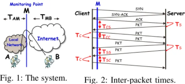
Fig. 1: The system.

Client Server M SYN SYN-ACK ACK PKT TCS PKT PKT TCC PKT TSS TSC PKT PKT TS TC TC TS

Fig. 2: Inter-packet times. filtered out. We show that the inter-packet time is a meaningful parameter to identify applications and that the precision of the classification increases from 80% to 98% for all applications after filtering the noise.

The rest of the paper is organized as follows. Section II dis-cusses the inter-packet time and present our model. Section III review our method and its application to the inter-packet time. Section IV and Section V describe the traces and the evaluation results respectively. Section VI concludes the paper.

II. MODELDESCRIPTION

In this section we analyze the inter-packet time and its use as parameter to classify Internet applications. Most of the recent literature in traffic classification [5]–[8], [10] argues that the inter-packet time is not an informative parameter to characterize and distinguish between applications. Indeed, the timing between subsequent packets is not only function of the application data availability, but also of the size of the TCP congestion window and the network conditions. Starting from these observations, we interpret the inter-packet time and model it to filter out the noise and to extract the time introduced by an application. This latter component is specific to each application and should resist better to network conditions. We present our model for a TCP connection, which can also be applied to UDP Internet traffic. We discuss possible differences at the end of the section.

In our model and without loss of generality we consider a monitoring point at the edge of the network, located in the ISP network, as shown in Figure 1. The monitor passively captures the flows between any two users; a flow consists of the packets with the same 5-tuple (IP source and destination, port source and destination, IP protocol). For each flow, we consider a client and a server, and we assume that the client is the user who initiates the connection, e.g., by sending the SYN packet for TCP. The packets of this same flow are inspected to extract the statistical properties to identify the application. In the following we model the system by considering the position of the user with respect to the monitor. Then we analyze the different cases when the host close to the monitor (A in Figure 1) acts as a client or as a server.

Figure 1 shows the three entities and their relative positions where A is the user behind the local network, B is an Internet user far from the local network, and M is the monitoring point. We defineTAM as the time taken by a packet to travel between the local user A and the monitoring point M and TM Bas the time between the monitoring point M and the user B. These times are shown in Figure 1.

The inter-packet time is characterized by the network, the size of the congestion window, and the time required by the application to generate and push the data to the transport layer. The inter-packet time computed at the monitor between any two packets of the same flow can take one of these four different forms, as shown in Figure 2:

• TCC is the time between two consecutive packets gener-ated by the client;

• TCS is the time between a packet from the client and a packet from the server;

• TSC is the time between a packet from the server and a packet from the client;

• TSS is the time between two consecutive packets gener-ated by the server.

We can now define the time taken by the application at the hosts A and B to generate the packets: TC and TS are the time due to the application at the client and server side respectively. The time due to the change of the network conditions, e.g., variable queueing time, between subsequent packets is accounted as ǫ.

Let’s first consider the communication between a client and a server, when the client is the entity A in Figure 1, i.e., located close to the monitor. From Figure 2, we can calculate the inter-packet times.TCC is equal to the timeTC, taken by the application to generate the data, plus the time ǫC due to possible changes of the network conditions between the client and the monitoring point.TCSis equal to the application time at the server TS plus twice TM B, the time for the packet to travel between the monitoring point and the server, and ǫS, which accounts for possible variations in the network conditions. The other times can be computed in a similar manner.

TCC = TC+ ǫC

TCS= TS+ (2 ∗ TM B) + ǫS (1) TSC = TC+ (2 ∗ TAM) + ǫC

TSS = TS+ ǫS

When the monitor is located close to the server and the client is the entityB of Figure 1, we calculate the inter-packet times in the same way.

TCC= TC+ ǫC

TCS= TS+ (2 ∗ TAM) + ǫS (2) TSC = TC+ (2 ∗ TM B) + ǫC

TSS= TS+ ǫS

The equations (1) and (2) show that many components con-tribute to the inter-packet time. This increases the complexity in creating a statistical signature of an application solely on the inter-packet time. Indeed, the time required by an application to generate and transfer packets to the transport layer is masked by the fact that additional time is added due to the network conditions and the TCP layer.

We are now interested to isolate the time due to the applica-tion, which we have identified asTC andTS in equations (1) and (2). We assume that the time due to the changes of

network conditions between two consecutive packets ǫC or ǫS is negligible. We are aware that the network is not stable and that the queueing time at the routers might change or the packets might follow different paths, but we assume that the times, that add or subtract, compensate each other.

Finally we quantify the time between the entity A and the monitoring point,TAM, and the time between the entityB and the monitoring point,TM B. We only discuss the case when the monitoring point is located close to entity A; the other case is similar. If we consider that the monitoring point is located close to the gateway router of the ISP, then TAM is half the local round-trip time that a connection experiences within the components inside the ISP. TM B is half the remote round-trip time over the wide area Internet from the monitoring point to the server [11]. Now the final question remains the estimation of the local and remote RTT to compute TAM and TM B. We compute the remoteRT T from the TCP three-way handshake to establish the session. We use the time between the SYN and the SYNACK packets, as this time is independent from the application, and we assume that it is constant for the duration of the session. Possible variations of the remote RTT are accounted in ǫS. The local RT T can be estimated from the SYNACK and ACK packets (or DATA packet in case of piggybacking).

Assuming that ǫC andǫS are negligible, we can filter any possible noise. Indeed, we can compute TC and TS from equations (1) and (2) to characterize an application and to classify the Internet traffic. Note that the same model applies to UDP traffic when we can estimate the local and remote RTT for a connection between the client and the server.

III. METHODDESCRIPTION

Our purpose for the classification of Internet traffic is to detect online which flow belongs to which application. We use a statistical and iterative method that computes the probability that packets are generated by an application. We have defined and used this method to classify Internet traffic based on the size of the packets [9]. When applied to inter-packet time, the method allows an iterative classification of the flows for each inter-packet time independently. It considers more inter-packet times until the classifier reaches a predefined threshold. Each flow corresponds to a sequence ofN + 1 packets P ktk, where k indicates the position of the packet in the flow independently of its direction. IP Tk with1 ≤ k ≤ N represents the inter-arrival time between P ktk−1 andP ktk.

In this section we first propose an overview of our method and then we detail its application and extension to the inter-packet time, which we use as a feature for determining an application signature. The method consists of three main phases which are detailed in the following sections: the model building phase, the classification phase, and the application probability or labeling phase.

A. Model building and classification phase

We use K-Means as supervised machine learning algorithm to partition the input in a predefined number of clusters. Given

the number of clusters, K-Means assigns each input feature to a cluster so as to minimize the Euclidian distance of each input from the centroid of the cluster.

IP Tk denotes the inter-packet time, i.e., the observations, and for each inter-packet time we train separately K-Means to obtain different set of classes. Each observation is pre-processed to determine the features in accordance with the4 different types of inter-packet time defined in Section II:TCC, TCS,TSC, andTSS. Figure 3 shows the observations as points in a two dimensional plane, where the X and Y coordinates indicate the first packetP ktk−1 and the second packet P ktk that determine the inter-packet time respectively. The absolute value of the point coordinates is equal to IP Tk. The sign of each coordinate depends on the type of inter-packet time: positive sign when one of the two packets that determines the inter-packet time is sent by the client; negative sign in case the packet is originated by the server. As a result of this processing phase, each feature is a2-dimensional vector.

In the learning algorithm, every class is affected by all applications with different probabilities proportional to the number of flows from each application present in the class. Hence, each class defines the probability that the elements within this class are generated by the applications.

The model building consists of constructing these sets of classes (clusters) by using a training data set, described in Section IV. This learning phase is used to computeP r(i/I), the per-class(i) probability knowing the application (I). We build a separate model, i.e., set of classes, for every inter-packet time noted by IP Tk and we use these classes for the classification phase.

The classification consists of using the classes defined in the learning phase to test and assign the Internet flows to a class. The test is performed by computing the Euclidian distance that separates the point defined by the feature extracted from the inter-packet time IP Tk and the centroid of each class determined for thek-th inter-packet time. We affect the point to the closest class. The test is repeated for all the inter-packet times of a flow iteratively until we reach a predefined threshold. The classification’s result consists in the probability that theIP Tk identifies an application and it is given as input to a labeling function described in the following section. B. Application probability or labeling phase

In the labeling phase we assign a flow to an application knowing the result of the classification. We combine iteratively the results of the classification for each single inter-packet time and we calculate the probability (P r(I/Result)) that a flow belongs to an application I given the classification results of the firstN packet times (i.e., class i(1) for the first inter-packet time, classi(2) for the second inter-packet time and so on). P r(I/Result) = P r(I) ∗ QN k=1P r(i(k)/I) PA I =1P r(I) ∗ QN k=1P r(i(k)/I) (3) P r(I) is the probability that any flow randomly selected comes from application I. The network administrator can set this value if he wants to put confidence on the classification derived

TCC TCS TSC TSS |IP T | |IP T |

Fig. 3: Types of inter-packet timeIP Tk as input to K-Means

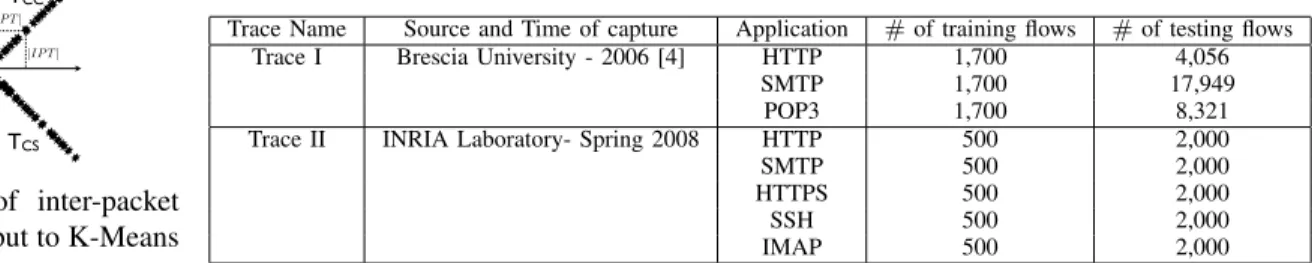
TABLE I: Traces Description

Trace Name Source and Time of capture Application # of training flows # of testing flows Trace I Brescia University - 2006 [4] HTTP 1,700 4,056

SMTP 1,700 17,949 POP3 1,700 8,321 Trace II INRIA Laboratory- Spring 2008 HTTP 500 2,000

SMTP 500 2,000

HTTPS 500 2,000

SSH 500 2,000

IMAP 500 2,000

by other techniques, such as port number classification. In our study, we consider this probability to be uniform for all applications.P r(i(k)/I) is the probability that IP Tkof a flow belongs to the classi knowing the application I. A is the total number of applications. We call this probability the assignment probability and we use it to decide on how well the profile of an inter-packet time of a new flow fits some applicationI. We calculate this probability for every inter-packet time computed after capturing packets from a flow. We stop this iterative process when the highest assignment probability is above a predetermined threshold or the maximum allowed number of tests is reached. This way the threshold is seen as a way to leave the classification phase earlier when we are sure about the flow.

IV. TRACEDESCRIPTION

In our analysis we use two real traces, see Table I. The first trace, noted Trace I, has been collected at the edge gateway of the Brescia University’s campus network [4] and the second trace, noted Trace II, has been collected at the edge of the INRIA Sophia Antipolis Network. The traces already indicate the type of application associated with each flow. In this way we can calibrate our supervised machine learning algorithm and we can evaluate our method. Trace I uses a method based on deep packet inspection to infer the real application. For Trace II, we separately collect the traffic from servers dedicated to unique applications hosted at the INRIA Network. For the evaluation of our method we only use the applications available in these traces, reported in Table I. However, our model is general and it can be applied to any application.

The flows of the traces are divided into a training and a testing set. The training set is used in the learning phase to construct the model and the testing set is used to evaluate how well our iterative method behaves in identifying the application. Note that we use the same number of flows per application to ensure that there is no bias in our learning phase.

V. EXPERIMENTALRESULTS

In this section, we evaluate the overall performance of our method while using the inter-packet time as a feature to classify the Internet traffic. We use the traces described in Section IV and we model the inter-packet time as discussed in Section II. The monitoring point is close to the client for Trace I and close to the server for Trace II, see Figure 2. We initially test the inter-packet time without filtering the noise and then we compare these results with the ones obtained by filtering the remote round-trip time from the TCS (Trace I) or the TSC (Trace II). We consider the local round-trip time

negligible because the traces are collected at the campus router for Trace I and at the servers for Trace II. The metrics used for the evaluation are:

• False Positive (FP) rateis the percentage of flows of other applications classified as belonging to an applicationI. • True Positive (TP) rate is the percentage of flows of

application I correctly classified.

• Precisionis the ratio of flows that are correctly assigned to an application,T P/(T P + F P ). The overall precision is the weighted average over all applications given the number of flows per application.

We run the test for all the available inter-packet times to test its significance as a feature for identifying applications. We set the number of clusters equal to400 for K-Means. We have tested the supervised machine learning algorithm with different number of clusters and400 gives the best results as it allows to group the features in small clusters and account for possible noise in the observations. The number of flows per application used for training and testing the algorithm are reported in Table I. We report the detailed results of the test conducted on the Trace I and only a summary of the results on Trace II for comparison.

Figure 4 shows the TP rate for the HTTP, POP3, and SMTP applications (Trace I) as a function of the number of inter-packet times considered for the classification without filtering the remote RTT. We can notice that the TP rate increases as we use more inter-packet times for the identification of the application for HTTP and SMTP traffic. However, the TP rate for POP3 traffic does not show any improvement, if not the results are worse after the IP T8. The variability of the TP rate for the first packets is associated with the noise added to the inter-packet time by the network conditions and the TCP behavior, as explained in Section II.

In Figure 5 we plot the FP rate for the traffic of Trace I as a function of the number of inter-packet times. We can observe that the FP rate drops below5% when we use more IP T s for POP3 and SMTP traffic, and it remains around 20% for the HTTP traffic. This means that some of the traffic of other applications is classified as HTTP. In particular, we can conclude from Figures 4 and 5 that part of the POP3 traffic is classified as HTTP traffic. Indeed, the IP Tk, with k ≥ 8, does not add significant information and the distribution of the inter-packet time for HTTP might have similar characteristics as for the POP3 traffic.

Now we preprocess the inter-packet time to filter the remote RTT and to eliminate part of the noise caused by the network. We test the method on the same traces (Trace I). Figure 7

Trace I 40 50 60 70 80 90 100 0 2 4 6 8 10 12 14 16 18 True Positive Inter-Packet time Web Trace I POP3 Trace I SMTP Trace I

Fig. 4: TP rate without filtering

0 5 10 15 20 25 0 2 4 6 8 10 12 14 16 18 False Positives Inter-Packet time Web Trace I POP3 Trace I SMTP Trace I

Fig. 5: FP rate without filtering

60 70 80 90 100 0 2 4 6 8 10 12 14 16 18 Precision Inter-Packet time Web POP3 SMTP Overall

Fig. 6: Precision without filtering

40 50 60 70 80 90 100 0 2 4 6 8 10 12 14 16 18 True Positive Inter-Packets time Web Trace I POP3 Trace I SMTP Trace I

Fig. 7: TP rate after filtering RTT 0 5 10 15 20 25 0 2 4 6 8 10 12 14 16 18 False Positives Inter-Packet time Web Trace I POP3 Trace I SMTP Trace I

Fig. 8: FP rate after filtering RTT 60 70 80 90 100 0 2 4 6 8 10 12 14 16 18 Precision Inter-Packet time Web POP3 SMTP Overall 98 98.5 99 99.5 10 12 14 16 18

Fig. 9: Precision after filtering RTT

60 70 80 90 100 0 2 4 6 8 10 12 14 16 18 Precision Inter-Packet time Web HTTPS IMAP SMTP SSH Overall

(a) Without filtering

60 70 80 90 100 0 2 4 6 8 10 12 14 16 18 Precision Inter-Packet time Web HTTPS IMAP SMTP SSH Overall 98 98.5 99 99.5 10 12 14 16 18 (b) After filtering RTT

Fig. 10: Precision (Trace II)

shows the TP rate and Figure 8 the FP rate. We can clearly see that the TP rate keeps increasing for all the applications when we add moreIP T s to the classification and approaches 97% after 12 IP T s. There is a significant improvement for the POP3 application already from the first few IP T s and after 6 IP T s we classify correctly more than 90% of the flows.

The FP rate also improves significantly for all applications and it equals5% already after the IP T6, see Figure 8. If we use more inter-packet times for the classification then the FP rate keeps decreasing and approaches1% for all applications when we use all available IP T s. This shows the efficacy of our filtering operation. Thus, we can conclude from this preliminary analysis that filtering the network noise from the inter-packet time is an important parameter to differentiate between applications.

In Figures 6 and 9 we plot the precision of our method for Trace I before and after filtering the RTT respectively. We first compute the precision per application and then we calculate the overall precision by weighting the single precision by the number of flows per application. Figure 6 shows that the precision of our method approaches 80% for HTTP traffic while it is around 95% for SMTP and POP3 traffic. This is justified by the low false positive rate obtained for these two applications (see Figure 5). After filtering the RTT we achieve a precision of 99% in all cases, see Figure 9.

We conclude the evaluation by testing our method on Trace II, see Table I. We plot in Figure 10 the precision of our method before (a) and after (b) filtering the RTT value. The results confirm the strength of our model in extracting relevant information from the inter-packet time to identify Internet applications. Finally, we can notice that filtering the RTT improves significantly the classification and we are able to

have a precision above90% already after few IP T s. VI. CONCLUSION AND FUTURE WORKS

In this paper we study the inter-packet time and we analyze how it can be used to identify Internet applications. We model the different components of the inter-packet time and we propose to filter the noise due to the network delay to extract relevant features for the classification. We then present our iterative method [9] already used for the classification based on the packet size and apply it to the inter-packet time.

We evaluate our solution on two different real traces and the results show that the inter-packet time is a relevant parameter to identify Internet traffic after some appropriate processing. In particular, when we filter the network noise from the inter-packet time, our method reaches a total precision of 99% for the classification of all applications. For future work, we want to test our method on other applications and we plan to combine the classification based on the packet size and the inter-packet time to build a very robust method for the identification of Internet traffic.

REFERENCES

[1] A. Moore and K. Papagiannaki, “Toward the accurate identification of network applications,” in the 6th PAM, October 2005, pp. pages 41–54. [2] A. W. Moore and D. Zuev, “Internet traffic classification using bayesian analysis techniques,” Perform. Eval. Rev., vol. 33:1, pp. 50–60, 2005. [3] J. Erman, A. Mahanti, and M. Arlitt, “Internet traffic identification using

machine,” in 49th IEEE GLOBECOM, San Francisco, USA, 2006. [4] M. Crotti, M. Dusi, F. Gringoli, and L. Salgarelli, “Traffic

classifica-tion through simple statistical fingerprinting,” in ACM-Sigcomm CCR, vol. 37, January 2007, pp. 5 –16.

[5] L. Bernaille, R. Teixeira, and K. Salamatian, “Early application identi-fication,” in CoNEXT, Lisboa, Portugal, 2006.

[6] S. Z, T. Nguyen, and G. Armitage, “Self-learning ip traffic classification based on statistical flow characteristics,” in the 6th PAM, 2005. [7] C. Wright, F. Monrose, and G. M. Masson, “Hmm profiles for network

traffic classification,” in ACM VizSEC/DMSEC, 2004.

[8] H. Kim, K. Claffy, M. Fomenkov, D. Barman, M. Faloutsos, and K. Lee, “Internet traffic classification demystified: myths, caveats, and the best practices,” in ACM CoNEXT, Madrid, Spain, 2008.

[9] M. Jaber and C. Barakat, “Enhancing application identification by means of sequential testing,” in IFIP-TC 6 NETWORKING, 2009.

[10] S. Zander, T. Nguyen, and G. Armitage, “Automated traffic classification and application identification using machine learning,” in LCN, 2005. [11] G. Maier, A. Feldmann, V. Paxson, and M. Allman, “On dominant