Changing mass applications in an advanced time domain ship motion program

(1)

Changing Mass Applications in an Advanced Time Domain

Ship Motion Program

by

Paul Richard Wynn

B.S., Virginia Tech (1986)

Submitted to the Department of Ocean Engineering

in partial fulfillment of the requirements for the degree of

Naval Engineer

at the

MASSACHUSETTS INSTITUTE OF TECHNOLOGY

June 2000

o

2000 Paul R. Wynn. All rights reserved.

The author hereby grants to MIT permission to reproduce

and to distribute publicly paper and electronic

copies of this thesis document in whole or in part.

Signature of Author ...

...

...

Department of Ocean Engineering

22 May 2000

C ertified by ...

...

Dick K.P. Yue

Professor of Hydrodynamics and Ocean Engineering

Thesis Supervisor

A ccepted by ...

...

Nicholas M. Patrikalakis

Kawasaki Professor of Engineering

MASSACHUSETTS I STITUTE Chairman, Committee on Graduate Students OF TECHNOLOGY _{Department of Ocean Engineering}

(2)

Changing Mass Applications in an Advanced Time Domain Ship Motion

Program

by

Paul Richard Wynn

Submitted to the Department of Ocean Engineering on 22 May 2000, in partial fulfillment of the

requirements for the degree of Naval Engineer

Abstract

Models are developed for a state-of-the-art time-domain ship motion program to predict ship motions during flooding and green water on deck events. Water mass from the flooding and green water is incorporated into the dynamic equations of motion using time-dependent mass and moment of inertia terms.

Green water on deck includes three subproblems: the problem of water shipping on deck, the problem of motion of water trapped on the deck, and the problem of water escaping off the deck. This research looks at the first two suproblems, both of which involve shallow water wave theory. Glimms method, also called the Random Choice Method, and the Flux Difference Splitting Method are both investigated as solution techniques for the motion of water on deck. This work provides a tool to estimate ship damaged stability and examine the effects of progressive flooding.

Thesis Supervisor: Dick K.P. Yue

(3)

List of Figures

2-1 Domain Definitions in the LAMP Mixed-Source Formulation . . . . 14

2-2 Coordinate Systems for LAMP Dynamic Solver . . . . 17

3-1 Compartmentation Model of a DDG51 Class Bow . . . . 25

3-2 Compartment Flooded Volume Model . . . . 27

4-1 Coordinate System for Two-Dimensional Free Surface . . . . 34

4-2 Initial Conditions for the Riemann Problem . . . . 38

4-3 Solution for Riemann Problem Case I . . . . 39

4-4 Solution for Riemann Problem Case II . . . 40

4-5 Solution for Riemann Problem Case III . . . 41

4-6 Solution for Riemann Problem Case IV . . . 41

4-7 Riemann Problem Solution Using Flux Difference Splitting Method . . . 42

4-8 Riemann Problem Solution Using Random Choice Method . . . 44

4-9 Solution Randomness in Random Choice Method . . . 44

4-10 Geometry and Variables for the Water Shipping Model . . . 45

4-11 W ater Shipping . . . . 47

4-12 Weatherdeck Division for LAMP Green Water Model . . . . 49

4-13 Flow Visualization of Green Water on Deck . . . 51

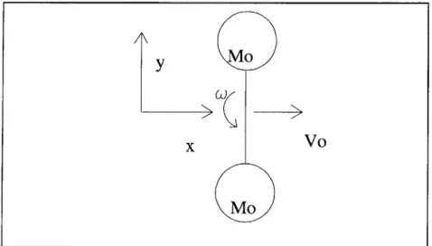
5-1 Model Used to Validate Dynamic Equations of Motion Solver . . . . 52

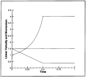
5-2 Conservation of Linear Momentum . . . . 53

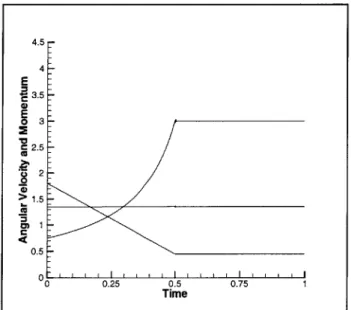
5-3 Conservation of Angular Momentum . . . . 54

(7)

5-5 5-6 5-7 5-8 5-9 5-10 5-11 5-12 5-13 5-14 5-15 5-16 5-17 5-18 5-19 5-20 5-21 5-22 5-23

Shallow Water Sloshing Below Resonant Frequency .

Shallow Water Sloshing, Twice Resonance Frequency

Roll Motion Intact and Flooded Ships . . . .

Sloshing Effects on Roll Motion . . . .

Pitch Motion Intact and Flooded Ships . . . .

Heave Motion Intact and Flooded Ship . . . .

Flooding Forward, Bow Height Above Free Surface .

Effects of Linear Hydrodynamics and Flooding . . .

Effect of Center of Gravity Shift on Pitch Motion . .

Progressive Flooding Pitch and Heave Motion . . .

Progressive Flooding Relative Bow Height . . . .

Linear and Nonlinear Progressive Flooding Pitch Mot

Linear and Nonlinear Progressive Flooding Relative B

Effects of Green Water on Pitch Motion . . . .

Effects of Green Water on Heave Motion . . . .

Relative Bow Height and Green Water Mass on Deck

Mass on Deck Using Different Shipping Water Velocit

Green Water Mass on Deck and Mass Center . . . .

Pitch Motion and Local Green Water Deck Loads . .

. . . 56 . . . 57 . . . 59 . . . 59 . . . 60 . . . 60 . . . 63 . . . 63 . . . 64 . . . 64 . . . 65 ion Calculation . . . . 65 ow Height Calculation . . . 68 . . . 68 . . . 69 . . . 69 ies . . . . 70 . . . 70 . . . . 71 A-1 Parallelepiped . . . . A-2 Rotation of Coordinate Systems . . . . B-1 Initial Conditions for the Riemann Problem . . . . B-2 Initial Conditions for Riemann Problem in Steady Velocity Frame B-3 Advancing Bore . . . . B-4 Case I, Coordinate System Translating at Vo . . . . B-5 Case II, Fixed Coordinate System . . . . B-6 Case III, Fixed Coordinate Sysem . . . . B-7 Case IV, Fixed Coordinate System . . . . B-8 Case V, Fixed Coordinate System . . . .

. . . 77

. . . . 79 . . . . 81 . . . . 82 . . . . 83 . . . 85 . . . 87 . . . 89 . . . . 91 . . . 93

(8)

Chapter 1 Introduction

1.1 Background

There are many hazards to ships that can result in hull damage and subsequent flooding.

Depending on the extent of a ship's damaged condition, flooding may cause a loss of buoyancy, a loss of transverse stability, and significant changes in trim and list. Adverse buoyancy and

trim conditions can lead to sinking by foundering, while the loss of transverse stability can lead

to capsizing. Significant trim and list changes may also result in water on the weatherdeck due

to shipping water as freeboard is lost. The water on deck, often referred to as green water or

the green water problem, can further harm a damaged ship's stability condition and also affect

the main hull girder loads, and deck and superstructure loads.

The state of stability, list, and trim in a damaged ship is dynamic; it varies over time as

the flooding event progresses and also depends strongly on environmental conditions such as

sea state and wind. Current naval standards, however, take a static approach in specifying

stability requirements for a damaged ship. For example, the naval standard DDS-079, reference

[5], requires that stability be analyzed on the equilibrium position of the damaged ship based purely on static geometry after the flooding event is complete. This analysis is similar in

many respects to intact stability calculations except with characteristics such as metacenter, center of gravity, and righting arm curves adjusted due to the weight of water in the flooded

compartments. Reference [5] makes use of wind speed and wave height for damaged stability

(9)

through applying steady wind healing moments and placing limitations on bulkhead opening

locations. Reference [9] refers to such bulkhead locations as "V-lines."

In [31] Surko points out limitations due to the static approach of current damaged stability

analysis procedure and criteria. Of these limitations, two are becoming more salient as the US

Navy shifts to performance based requirements. First, in 1987 the Chief of Naval Operations

(CNO) [24] endorsed a series of operational characteristics to be incorporated into surface

combatants of the year 2010. Included in these characteristics is that a ship has the capability

to fight, even though it may have sustained hull damage and be flooded, with whatever weapons

systems are available. To assess whether a ship could employ weapons while fighting hurt would

require analyzing ship motions which is well beyond the scope of reference [5] procedures. In fact

references [14], [15], and [16] report there is no information in the literature and no appropriate

computer prediction tools to assess ship motion performance of partially flooded or flooding

ships in waves and wind. The second significant limitation in current damaged stability criteria

pointed out by Surko is that moderate wind and sea conditions are assumed. In reference [31]

Surko shows there is a considerable probability of experiencing wave action that exceeds the

moderate 8 foot wave height assumed in reference [5].

As a first step in addressing these limitations, model tests have been performed to assess

the dynamic stability of current fleet combatants in a damaged condition. These tests were

reported in references [14], [15], and [16]. The term "dynamic stability" in these model tests

is meant in its true sense: actual ship motions and ability to withstand sinking under a variety

of environmental and flooding conditions.

Model testing can be costly due to production of scale models and the use of large

labora-tory facilities for the experiments. Also, the time requirements to prepare and conduct model

tests make it difficult to use testing early in the design process to predict damaged dynamic

stability for immature designs and design variants. Development of damaged stability computer

prediction tools, especially for early in the design process, would be ideal as a supplement or

replacement to model testing.

Computational fluid dynamic (CFD) codes that predict ship motion would provide a good

foundation for development of damaged stability prediction tools. Of the two general categories

(10)

approach is better suited for damaged stability analysis. Frequency domain codes only consider

the mean underwater hull form and linearize by assuming small wave and motion amplitudes.

The linear prediction would breakdown under high sea states and large amplitude responses

that need to be considered for a damaged stability analysis. On the other hand, state of the

art CFD codes that predict wave-induced ship motions and loads in the time domain solve

the non-linear three-dimensional ship motion problem and can handle large wave and motion

amplitudes.

Also, inherent in use of a time domain code as a damage stability prediction tool is the

ability to predict motions during the entire flooding event. Such a tool would be useful

at assessing the effects of progressive flooding. Progressive flooding occurs when water in

flooded compartments floods into adjacent compartments by overflowing watertight bulkheads

or leaking through damaged bulkheads. The R.M.S. Titanic sank as a result of progressive

flooding which flooded compartments beyond those originally opened to the sea by the

iceberg-caused damage. Progressive flooding is of special concern in warships where hull damage from

combat is likely to cause the watertight bulkheads surrounding the affected compartments to

suffer some damage from shock or fragmentation. The US Navy has an interest in progressive

flooding but the published work to date, an example of which is in reference [2], has been simple

quasistatic models that do little more than determine the damaged ship hydrostatic position

throughout the progressive flooding event.

1.2 Research Objectives

This research investigates the addition of a compartment flooding model and green water model

to a CFD code that predicts ship motions in the time domain so that it can be used as a

damaged stability prediction tool. There is no effort made by the author to perform damaged

stability analysis. The specific CFD code used for these purposes is the Large Amplitude

Motions Program (LAMP) developed by the Ship Technology Division of Science Application

International Corporation (SAIC). The theory and some results of the LAMP code have been

presented in several papers including references

[7],

[26], and

[19].

A brief review of the theory

(11)

Green water and compartment flooding can be considered as events that, at each instant, are part of the ship and change the total rigid body mass and mass distribution. Sloshing and

water motion will also affect the mass distribution. Both events are fundamentally the same

process that can be modeled as a time-rate-of-change of ship mass in the rigid body motion

problem. The approach in this thesis, then, is to calculate the affect on ship motions from green

water and flooding by incorporating time-dependent mass and mass moment of inertia into the

LAMP dynamic equations of motion solver.

The green water problem includes three subproblems: water shipping; motion of water on

deck; and water escaping off deck. This research looks at the first two subproblems in some

detail. Water escaping is treated by simply letting water fall off the weatherdeck edges.

The water motion on deck subproblem involves shallow water wave theory. There are

several solution techniques that have been developed to solve the shallow water wave problem.

Two of the techniques, Glimms method (also called the Random Choice Method) and the Flux

Difference Splitting Method, are robust in the sense that they can handle dicontinuities such as

shocks and bores in the solution. This research investigates implementation of both solution

techniques. As a result, the flux difference splitting method is selected as the solution technique

(12)

Chapter 2 LAMP Description and

Development of Equations of Motion

2.1 LAMP Description

This description of LAMP is primarily based on information from reference

[211.

LAMP com-putes a time domain solution for a general three-dimensional body floating on a free surface.

Six degree-of-freedom motions are permitted. LAMP obtains a potential flow solution to the

body-wave interaction problem using the boundary-element (or panel) method where the

sub-merged body surface is divided into a number of panels. The incoming waves can take any

form. At each time step the hydrodynamic pressure forces on the hull, which are computed

from the complete velocity potential solution, are combined with body forces and any external

forces to solve the equations of motion. The hull pressure forces may also be used to calculate

hull bending and torsional moments and shear forces.

In order to balance computation requirements with physics correctness and complexity, LAMP has three methods of calculation. The user selects a specific calculation method for a

LAMP run through control variables specified in the input. The LAMP calculation methods

(13)

Method Hydrodynamic, Restoring, and Froude-Krylov Wave Forces

Free Surface Boundary Condition on Mean Water Surface

LAMP-1 3-D Linear Hydrodynamics

Linear Hydrostatic Restoring and Froude-Krylov Wave Forces

Free Surface Boundary Condition on Mean Water Surface

LAMP-2 3-D Linear Hydrodynamics

Nonlinear Hydrostatic Restoring and Froude-Krylov Wave Forces

Free Surface Boundary Condition on Incident Water Surface

LAMP-4 3-D Nonlinear Hydrodynamics

Nonlinear Hydrostatic Restoring and Froude-Krylov Wave Forces

Table 2.1: LAMP Calculation Methods and Description

The LAMP-4 method is the complete large-amplitude method where the 3-D velocity

po-tential is computed with the linearized free-surface condition satisfied on the surface of the

incident wave. Both the hydrodynamic and hydrostatic pressure are computed over the

in-stantaneous hull surface below the incident wave surface. The incoming wave slope must be

small. Small slope generally indicates that the wave height is one order of magnitude less than

the wavelength. LAMP-4 has large computational requirements and has traditionally been

run on a supercomputer. However, the mixed-source formulation now used in LAMP to solve

the potential flow problem provides enough computational savings for LAMP-4 to be run on a

workstation. The mixed source formulation is discussed later in this chapter.

The LAMP-2 method is an approximate nonlinear method which retains many of the

ad-vantages of both LAMP-1 and LAMP-4. It uses a linear 3-D approach like LAMP-1, where

the potential flow problem is solved over the mean body boundary position, to compute the

hydrodynamic (radiation, diffraction, and forward speed) part of the pressure forces. The

hydrostatic restoring and Froude-Krylov wave forces are calculated on the portion of the ship

beneath the incident wave surface. The requirements for computer resources are about the

same as LAMP-1. Note that the LAMP-2 and LAMP-4 nonlinear methods are based on the

approach that both the ship motions and the waves may have large amplitudes.

The LAMP-1 method is the linearized version of the LAMP-4 method with the free surface

(14)

restoring forces are computed from waterplane quantities while the Froude-Krylov wave forces

are calculated with pressure below the undisturbed free surface location. Like LAMP-2, the

mean body boundary position is used for the potential flow problem.

LAMP uses two approaches toward solving the hydrodynamic problem for the potential

function <D(t) at each time step: a direct solution of the hydrodynamic potentials in the time

domain and a solution using pre-computed impulse response functions. Both solutions are based

upon a mixed-source formulation that is briefly described in the remainder of this section.

In the mixed-source formulation, both the Rankine source and the transient Green function

are used. The fluid domain is divided into an inner domain I and an outer domain II as shown

in figure 2-1.The inner domain is enclosed by the wetted body surface Sb, a local portion of the

free surface Sf, and the matching surface Sm. The free surface

Sf

intersects the body surface and is truncated by the matching surface Sm.at the water line Fm. The outer domain is the

rest of the fluid region enclosed by Sm, an imaginary surface So, and the remaining free surface

intersected by Sm.and S,.

S,

Figure 2-1: Domain Definitions in the LAMP Mixed-Source Formulation

The fluid motion is described by a velocity potential,

(15)

where 4)w is the incident wave potential and 4F is the total disturbance potential due to the

presence of the ship. ' is a position vector and t is time. In the inner domain I, the initial

boundary value problem for D = (D can be expressed as,

V2_4,_{= 0} _{in I} _(2.2)

The inner domain potential must satisfy the free surface and body boundary conditions. The

free surface boundary condition is linearized in all three formulations, such that

a2 +g2L =0 on Sf(t),t >0 (2.3)

where g is the gravitational acceleration. The body boundary condition is next applied on the

instantaneous underwater body for LAMP-4 and the mean underwater body for LAMP-1 and

LAMP-2,

=

V

a-- on Sb(t),

t > 0

(2.4)

Sn n

where n is a unit normal vector to the body out of the fluid and V n is the instantaneous

body velocity in the normal direction. Sb(t) is constant for LAMP-1 and LAMP-2. Finally,

the initial conditions require a zero disturbance potential on the free surface at t = 0,

a5I

D 0 at t = 0 (2.5)

at

The corresponding boundary integral equation in terms of the Rankine source is,

27r41(P) +

L

('JGn - (I1nG)dS = 0 (2.6)

where C = 1/r =

1/IP

-

Q1.

P = (x, y, z) and

Q

= ((,riC) are the field point and source

point on S, = Sf U Sb U Sm.

In the outer domain II, the initial-value boundary problem for (D =

#D1

can be written as,

V24J 1 1 = 0 in II (2.7)

at

2 _+g

_az

₌₀ _on _{Sf(t),t >0} _(2.8)

(16)

VIDII -+ 0 at

oo

)11-

_at

=0 at t = 0 (2.9)

The corresponding boundary integral equation in terms of the Rankine source is,

27rJII(P)

+

j

(41 1G - J

)InGO)dS

1 = M(P, t) (2.10)

JSm

where the memory function M(P, t) is defined as,

M(P, t) = dr

{Im(

1 1G - Q)4Gf)dS 1 1 + - (D1Gf- - 4DrG{)VN dL (2.11)

where Im is the water line of the matching surface, VN is the normal velocity of 1m, and G' and Gf are associated with the transient Green function. Reference [29] provides a detailed description of the transient Green function.

The matching surface is treated as a control surface and moves with the body. To complete the problem statement, the matching conditions require that the total disturbance velocity potential and the normal velocity across the matching surface are continuous, thereby producing

4) = 11 on Sm (2.12)

aQ1 _ a _{1 1}

=4)-

an

on Sm (2.13)

cBn

c8n

The solution is obtained at each time step. Using the panel method, the above equations

are used to solve for 4), on

Sb,

2L on S, and 4), and 0' on

Sm.

Bernoulli's equation is used

to compute the pressure on the hull surface, which is integrated to get the hydrodynamic forces on the ship. Then the linearized free surface boundary condition can be used in domain I to integrate in time and update the values of the total disturbance wave elevation and 4)j at the next time step.

(17)

2.2 LAMP Rigid Body Dynamics

This section outlines the solution in LAMP to the rigid body dynamic problem. Several

coordinate systems, illustrated in figure 2-2, are used to describe the six-degree-of-freedom

motion of a ship in a seaway. The global system ,Og, is fixed on earth. A second system is

the local system, 0/, which is fixed at the ship's center of mass, cg, and rotates with the ship.

The relation between these two systems is by the position vector, R, and a set of euler angles,

Q = ((Dr,

E,

T), measured in the global system and following the sequence of rotation T,

E,

and 4r, respectively, fromOg to

O/.

The angles

I

can be thought of in common terms: IQ is

z

VoO'

Og---)

Figure 2-2: Coordinate Systems for LAMP Dynamic Solver

the ship's yaw , 9 is the ship's pitch, and -(r is the ship's roll. The matrix L is the euler angle

transformation matrix between Og and.0/.

cos T cos E sin T cos E - sin

1

L -sin T cos 4br

+

cos 4 sin E sin (r cos T cos 4)

+

sin T sin E sin 4r cos E sin 4r sin T sin r

+

cos I sine cos 4r - cos T sin 4r

+

sin T sin E cos <Dr cos E cos br

(2.14) A third coordinate system, Og',has the same orientation as Og but is initially centered at cg

(18)

to define the rigid body geometry, for example the input and initial static systems, but these

are not necessary in describing the solution to the dynamic equations of motion.

Velocities for the dynamic problem are defined as follows. All linear velocities are referred

to the global coordinate system unless indicated. Vo is the velocity of a point on the rigid

body, or extended rigid body, that coincides with Og at time t; V is the rigid body velocity at

cg; Vg is the rigid body velocity at cg referred to the O' system. - is the absolute angular

velocity and .7Wi/ is the angular velocity in local system, O/. The velocities are related by

V = Vo + wx R (2.15) --+ d -- + V - R (2.16) dt Vg = Vo - Uship (2.17) W/ = Tw (2.18) - T- d -4 -T d _ w= L wi and -W =T -W (2.19) dt dt

The rate of change of Q in terms of the angular velocity of the ship,

U/,

is given by

Sn = [W ] U/(2.20) dt

where [W] is defined as

1 sin 4 r sin e/ cos E cos JDr sin E/ cos

1

[W] = 0 cos r - sin<Dr (2.21)

0 sin<DrD/ cos E cos <Dr

/

cos

I

To determine R and the dynamic equations for the rigid body motion must be solved.

The equation of motion for translation can be written as

+ d

-Fo = -((Mo)(V, - Uship)) (2.22)

dt

(19)

The equation of motion for rotation about cg in the local coordinate system can be written as

-~--d II __ -T--

-Mo = I I/-(w/) + L (V/ x Y/w/) (2.23)

where Mo is the total moment acting on the rigid body about cg in the Og or Og' coordinate

system and

1/

is the rigid body mass moment of inertia tensor in the local coordinate system. Fo and Mo are calculated from the instantaneous total force including hydrodynamics and

external contributions. Equations 2.22 and 2.23 can be formulated into a coupled system of

equations

E - - = q (2.24)

Combining equations 2.24, 2.16, and 2.20 yields

d [E71[q]

-- -+ _(2.25)

-+ [W] -4/

Equation 2.25 is solved by the fourth order Runge-Kutta method.

2.3 LAMP Rigid Body Dynamics With Time-Dependent Mass

The solution to the rigid body dynamic problem requires some modification to account for

time-dependent mass and mass moment of inertia tensor due to water added to a ship from

flooding or shipping water. Also, water motion will change the mass moment of inertia tensor

over time. This section provides a detailed formulation of the rigid body dynamics solution

with time-dependent mass and mass moment of inertia tensor.

2.3.1 Infinite Frequency Added Mass and Moment of Inertia

The solution to the rigid body dynamic equations of motion in LAMP makes use of the ship's

(20)

explains why they are used.

4

-LAMP calculates the total instantaneous force, Fo, and moment, Mo, for the ship rigid

body dynamic equations. Force and moment contributions from hydrostatics, the incident

wave, hydrodynamics, external forces, and body forces are used to calculate Fo and Mo. Due

to the total nature of the force and moment calculation the infinite frequency added mass and

moment of inertia for the ship are not required in the dynamic equations. However, they are

used in the LAMP rigid body dynamic solution for numerical stability.

The added mass and added moment of inertia terms are referred to the global coordinate

system when calculated. This causes them to be time-varying as the rigid body orientation

changes with respect to the global system. The added mass and added moment of inertia terms

are defined at an each time instant as

aij = p ji-dS i, j = 1, 2,..., 6 (2.26)

//

O#

B

where a = ni, i = 1, 2,3 and L= (an x n)i-3, i = 4, 5,6. Vector . is the position vector

on the body, B, in the local coordinate system and - the outward normal of the fluid on B.

The global added mass matrix, Ao, is a 6x6 matrix constructed with term i,

j

of Ao equal to

aij.

The terms in Ao are defined as 3x3 submatrices

Ao

Al A1 2 0 (2.27)

A

2 10 A220

2.3.2 Translation:

By replacing the rigid body mass matrix, Mo, with Mo + Am(t), the equation of motion for

translation can be written as,

Fo = -((Mo + Am(t))(V, - Uship)) (2.28)

(21)

For stability in the Runge-Kutta numerical integration scheme, added mass terms are added to

both sides of equation 2.28 to obtain

- A ( - - U

d

Fo+Ano (Vo) +A20() =-((Mo +Am(t))(Vo -AUship))+Ao-(Vo) +A 120-( w)

(2.29)

-4 -4 ₊

Rewrite equation 2.29 by substituting F for the left hand side where F Fo A1 1o(V) +

A12A _{1 2}_{ot( w)}

d - -+ 71-> d

F = ((Mo + -Em(t)) (Vo - Uship)) + A-o- (VO) + 0 A -(W (2.30)

then group terms and carry out differentiation to get the final form of the translation equation

of motion

-+ - d -Tr d ->d

F = (Mo + Am(t) + Ano)-(Vo) + A12oL T('/) + (Vo - Uship)-(Am(t)) (2.31)

2.3.3 Rotation:

The rotation equation of motion is expressed in the local frame

O/.

The local frame is used so that derivatives of I and T do not have to be calculated.

Definitions and relations:

Some terms need definition prior to developing the rotation equation of motion. I is the rigid

--4

body mass moment of inertia tensor in the Og or Og/ frame. H is the angular momentum

about

cg

in the Og or Og/ frame. H/ is the angular momentum about cg in the 0/ frame. The following equations relate the rotational terms:

--4

H = (2.32)

/ =/Y/ (2.33)

Mo/ =

TMo

(2.34)

(22)

Formulation:

The equation of motion for rotation about cg in the 0/ coordinate system can be written as, d -+4

Mo/ = -(H/) (2.36)

dt

In order to expand the term d (H /),the following equation, which is a standard result from any

dynamics textbook for vector derivatives in rotating systems, is used,

(A )= (A w) x A (2.37)

d d-+

In equation 2.37, A(A) is the absolute rate of change of A written terms of the unit vectors

in the rotating system, A (A)r is the rate of change of A as viewed from the rotating system,

and V is the absolute angular velocity of the rotating system. Placing the angular momentum

vector H/ into equation 2.37 gives,

d I d -+38

-(H/) = -(HI/), f/ x4' (2.38)

dt dt

The angular momentum as viewed from the rotating (local) system is,

(H-4/)r = 1/,/ (2.39)

inserting equations 2.33, 2.36, and 2.39 into 2.38 gives,

Mo/ = -(If/J/) + 'W/ x i/W/) (2.40) dt

Due to time varying mass, the rigid body mass moment of inertia tensor,I/, is replaced by

lo/

+

AD/(t). Applying equation 2.34 to 2.40 and making the substitution for the time varying inertia results in

LMo = -((Io/

+

AI/(t))D/) W/ x (o /+

AI/(t))L/)

(2.41) dt

(23)

Then, by performing differentiation and moving L to the right hand side equation 2.41 becomes

Mo = W

(o/+

AT/(t))

i/+

(AI/(t))U/

U/

x [(o+

AI/(t))

W/] (2.42)

Similar to equation 2.29, for stability of the numerical scheme, added mass terms are added to

both sides of the equation 2.42. Also, the substitution of M = Mo

+

A2 10o(V0) A22OA(Q)

is made so that

= ( o/+ AI/(t)) -/ + ( kL/())O/+ W/ x [o/ /())W/ + 210 VO) 220 ()

(2.43)

Finally, grouping terms gives the final form of the rotation equation of motion

M= A2 o (V [A220LT + r (Io/+ A/)(t)))] )/l+rd -T(./x [(To/ + AI/(t))W-/)

(2.44)

2.3.4 Coupled Rotation and Translation Equations:

The translational and rotational equations of motion, equations 2.31 and 2.44, are a coupled

system

E - - = q (2.45)

dt y

where

IAno+

Mo + Am(t) A122L.

E ] _= (2.46)

A2 10 A22OLT + LT(o + AII(t))

and

[

~

~F

(Vo - Us hip) (Em~t)(.

[-

]

(/

x (lo/ + AI/(t))J/i)) - u (Al/(t))

]

The details of [E], and [q] were not shown in equation 2.24. They contain terms similar to

equation 2.45 except that there are some new terms in equation 2.45 due to the time-dependent

mass and mass moment of inertia. The new terms are

(VO

-Uship) T(Am(t)) in the translation equation and T-i/A (A!/(t)) in the rotation equation. Also, mass and mass moment of inertia

(24)

Chapter 3 Models for Flooding

3.1 Compartmentation

Watertight internal subdivision using bulkheads to form compartments within a ship has been

the primary means of limiting the extent of flooding in a damaged ship. During ship design, various bulkhead arrangements are evaluated against operational and damaged stability

re-quirements to determine an optimal ship subdivision. In general, improved damaged stability

performance with increased subdivision must be balanced against drawbacks to

compartmen-tation such as weight, interference with arrangements, and access to systems.

The capability to compartmentalize hull geometry had to be added to LAMP in order to

model flooding for damaged stability analysis. Since this thesis is concerned with the basic

changes necessary to LAMP for it to be used as a damaged stability prediction tool, it was

considered adequate that the compartmentation model only use transverse bulkheads. If

required for a specific ship configuration or damaged scenario, more detailed compartmentation

model with longitudinal bulkheads and damage control decks could be added.

A LAMP program module was written to accept arbitrary transverse bulkhead locations

as input. The bulkhead locations are specified by their distance from the ship bow. The

distance is normalized through dividing by the overall hull length. Any number of bulkheads

can be created. The bulkhead locations are then automatically spliced into the hull geometry

description to form compartments that are bounded by forward and aft bulkheads, the hull, and

(25)

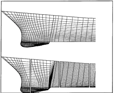
the place of a forward or aft bulkhead as applicable. Figure 3-1 illustrates compartmentation

of the bow of a DDG51 Class hull. In this figure the intersection of each line with other lines

Figure 3-1: Compartmentation Model of a DDG51 Class Bow

is described by an three dimensional coordinate point.

Consistency between the flooded volume calculation and the LAMP hydrostatic calculation

is important for an accurate representation of the ship's mean body position. Because the

compartmentation module uses the detailed LAMP hull geometry description to define the

majority of a compartment, the model provides excellent consistency between the compartment

flooded volume calculation and the hydrostatic calculation. Results were obtained for a ship's

final hydrostatic position after a flooding event. A comparison of the flooded volume against

the resulting change in ship displaced volume showed the two agreed to within 99%.

Finally, the compartmentation module is only used for calculations on the internal flooded

water and does not affect the hull geometry description. This is important because the hull

(26)

3.2 Calculations For a Compartment's Flooded Volume

For sloshing of a flooded volume of water it was conservatively assumed the water within a

rolling compartment maintains a horizontal surface. In actual ship compartments there are

generally some solid objects that will project through the surface of the water to reduce free

surface motion. Ship designers account for this effect through the surface-permeability factor.

The horizontal surface assumption produces a first order approximation for sloshing. For

simplicity, pitch motion was not considered in the flooded water sloshing calculations. Damaged

stability criteria mainly look at transverse stability while in a damaged condition and sloshing

due to pitch would have little-to-no effect on this stability. Ignoring pitch motion also made it

easier to check the accuracy of the flooded volume calculations.

Numerical solution techniques for calculating the instantaneous dynamic free surface in a

flooded compartment are an alternative to assuming a horizontal surface but they provide a

relatively small increase in accuracy compared to the significant increase in complexity and

calculation time. An actual ship compartment is outfitted and filed with equipment so even if

the instantaneous free surface were calculated it probably would not reflect the actual conditions

in the flooded compartment. Efforts to accurately calculate a free surface are better suited for

the shallow water flow problem that arises when shipping water.

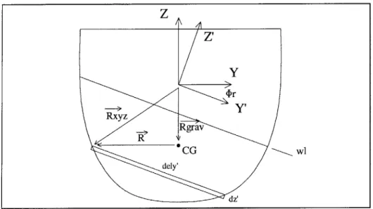
Figure 3-2 illustrates the instantaneous position of a flooded compartment volume with the

ship undergoing a roll to starboard with roll angle, <Dr. The roll is made through the ship's

center of gravity, cg. The unprimed coordinate system in the figure, the YZ system, is the

LAMP initial static system which is used as the reference to describe the hull and compartment

geometry through position vector Rxyz. The primed coordinate system has been introduced

for the flooded volume calculation and rotates to maintain the Y/ axis parallel with the water

surface.

Flooded compartment volume is calculated in the YIZI system by summing the rectangular

parallelepipeds of length dely/ and height dzl. These are indicated in figure 3-2 and have a depth

dx along the hull's longitudinal axis. The parallelepiped geometry was selected to simplify

moment of inertia calculation. The flooded volume calculation is initiated by converting the

(27)

Z

Y

<br -+ Y' Rxyz Rgrav CG w1 dely' dz'

Figure 3-2: Compartment Flooded Volume Model

between YZ and YIZI,

RI= Rz Rgrav) (3.1)

Since only roll motion is considered, the x and x/ values are the same. If it were desired to

include pitch motion in the sloshing model, the pitch angle could be included in ~C and the

calculation proceed in the same manner as described here. The summation for volume is made

over x using j = Jmax intervals and over z/ with k = kmax intervals where x spans the flooded

compartment length and z/ ranges from the minimum value to the waterline wl

Vcmpt = ( ( dely/dz/dx (3.2)

Xj Zik

At a fixed roll angle, the waterline value wl serves to determine compartment flooded volume. If a specific instantaneous flooded volume is desired for a particular flooding scenario, wl can be adjusted through an iteration process until the desired volume is reached.

The center of mass of a flooded compartment, CGcmpt = (X11, i 2, i/ 3), can be calculated where

/;i = xeii 1, 2,3 (3.3)

(28)

volume and center of mass known, forces, moments, and the time-dependent mass terms can

be calculated due to the flooded water and added to the dynamic equations of motion 2.45. If

the flood rate is specified it is used directly as the ((Am(t)) term in the equations of motion.

Otherwise A

(Am(t))

needs to be calculated based on the flooded volume time history.

The calculation for flooded water mass moment of inertia is made by summing the mass

moment of inertia of each parallelepiped about the flooded volume center of mass. Appendix

A outlines the method for doing this. After calculating the flooded volume mass moment of

inertia tensor about the center of mass, SMIcmpt, the parallel axis theorem and a rotational

transformation must be applied to refer SMcmpt to the ship's cg in the local coordinate system.

The instantaneous flooded volume mass moment of inertia tensor is used for the AI/(t) term

in the dynamic equations of motion. The

(AI/(t))

term must be calculated based on the flooded volume mass moment of inertia time history.

To better model an actual ship, compartment permeability could be used in the calculations

for a compartment's flooded volume. It would be a trivial matter to add permeability to the

calculations above.

3.3 Flooding Simulation

With the compartment flooded volume model established there are several approaches to

run-ning a time domain flooding simulation. First, the simulation can start with the initial condition

that the flooding event is complete and the ship is in its final flooded static condition. A

com-puter module was written to run this type of simulation. The module solves for a ship's final

static position after a flooding event in any specified compartments is complete. The module

uses an iterative procedure to calculate the final ship position and then revises the ship mass,

moment of inertia tensor, and

cg

location to account for the added water. Alternatively, the module can maintain the ship intact and provide the total water that would be added if specific

compartments were flooded. This information can be used as an upper bound on flooded

compartment volume if it is desired to flood the ship as time advances in the simulation.

The second approach for a time domain flooding simulation is to start with either an intact

(29)

simulation time progresses. This approach is what is referred to as progressive flooding in

Chapter 1. The mass addition rate from flooding would need to be specified in this type of

simulation. One technique to specify this rate is to specify a hull opening location due to

damage and let water enter the compartment when the instantaneous free surface is above the

hole. The flow through the hole of area A and at static head h would be governed by the

short tube orifice equation,

Q =

CdA/2~g?. Tables may be obtained for the coefficient Cd from textbooks on hydraulics such as LeConte [18]. In [6] Dillingham states Cd may be taken as

0.60 with very good accuracy.

3.4 Wind

LAMP is configured to include external forces in its calculation and currently has modules

that calculate external forces for items such as appendages, viscous roll damping, and moving

weights. It is a simple matter to include a heeling moment caused by beam winds using an

equation such as the following from reference [17]

M = K(Vw)2Al(cos(<D,))2 (3.4)

A

In equation 3.4 Vw is the wind velocity, A is the ship sail area, 1 is level arm from centroid of sail

area to half draft, 4r is the roll angle, and A is the ship displacement. K is a constant whose

value can vary depending on units used in the equation and on assumptions on values for wind

drag coefficient. Reference [17] contains a discussion on calculating wind heeling moments.

Equation 3.4 could be expanded to include the wind heading angle so that three dimensional

wind forces and moments on the ship are included in the LAMP calculation.

3.5 Causes of Loss of Accuracy in LAMP Flooding Simulations

When linear hydrodynamics are used in LAMP to solve the potential flow problem (LAMP-I and

LAMP-2) the initial mean body boundary position is used for the duration of the calculation.

However, due to sinkage and trim from flooding the actual mean body boundary position will

(30)

accuracy in the calculated ship motions will result.

One strategy to limit the loss of accuracy in a flooding simulation using linear hydrodynamics

is to select an intermediate body position between the intact and final flooded conditions.

Another approach would be to run the linear hydrodynamics LAMP simulation at the intact

body position and then at the final flooded body position and use the worse case ship motions

as the motion estimate. Of course, non-linear hydrodynamics (LAMP-4) could be used for

the flooding simulation but the penalty is that much more time is required to perform the

calculation.

As water floods into the ship it causes a time-dependent shift in the ship's center of gravity,

cg. This shift is not accounted for in the LAMP dynamic equations of motion solution. For a

small amount of flooding in a massive ship the shift in cg will be trivial. Under these conditions

the calculated ship motions would be reasonably accurate. However, as the magnitude of the

cg shift increases, the calculated angular ship motions will be wrong because the rigid body

moment determined at each time step grows in error.

Finally, when simulating significant hull damage such as a compartment size hole,

consid-eration should be given as to whether complete body panelization that assumes an intact hull

will provide an accurate enough hydrodynamic solution. A more accurate method may be to

(31)

Chapter 4 Models for the Green Water

Problem

4.1 Background and Scope of Green Water Model

As a flooding ship loses freeboard, the likelihood of shipping water increases. The water on

deck, in turn, can further degrade the ships stability condition. This is of special concern for

smaller vessels. A review paper on the subject of water on deck and stability of has been

published in reference [3]. Also, in reference [6], Dillingham provides calculations to show that

instabilities caused by excessive deck water may cause capsizing of small fishing vessels. The

green water problem can be decomposed into three subproblems: shipping water, water escaping

off deck, and the motion of water on deck. For adequate modeling of the green water problem

in a time domain ship motion program each subproblem must be addressed.

Most work reported on the green water problem has focused on the water motion on deck

subproblem. This emphasis over the other two subproblems is primarily due to

water-motion-on-deck sharing the same basic theory as that for flow of compressible gases. Specifically, the equations governing water motion on deck, equation 4.13, are derived from the theory for

waves in shallow water, covered in detail in reference [29], and are of the same form as the

compressible gas dynamics equations. The necessity in industry for dealing with the flow of

gases has resulted in numerical solution methods that can be directly applied to the

(32)

the water depth and horizontal particle velocity. Solutions to the governing equations can

involve discontinuities such as shocks, bores, and hydraulic jumps. Any numerical methods

used to solve the equations must be capable of treating discontinuities. Most of the numerical

methods fall into two general categories characterized by the scheme used to solve the governing

equations: the flux difference splitting method and the random choice method, also known as

Glimms Method. Both schemes handle discontinuities in the solution without any special

treatment and were evaluated in this thesis. The Random Choice method involves looking

at solution curves, called characteristics, to the governing differential equations. The flux

difference splitting method combines a finite difference method with characteristics. A different

approach to solving the water on deck problem is in reference [13] where the authors solve for

wave motion in a rolling tank using a finite difference scheme coupled with analytical techniques.

This approach illustrates the special care that must be taken with discontinuities with which

the numerical scheme is incapable of handling.

This chapter develops a green water model for the LAMP program in head seas. The two

main methods for solving the water-on-deck subproblem are evaluated for use in the model using

a two-dimensional free surface. A method for incorporating water shipping into LAMP is also

devised. The water escaping off deck subproblem is not formulated because a proper calculation

would require a three-dimensional free surface solution to the shallow-water problem. Three

dimensions would introduce transverse water velocities so that as the green water travels aft on

the weatherdeck it also moves towards the port and starboard deck edges and then over board.

The green water model used for this thesis only calculates longitudinal water velocities so green

water mass is removed from the weatherdeck by letting it fall off the after end of the portion

of the weather deck included in the computation. This is accomplished by setting boundary

conditions for the water-on-deck calculation to zero at the aft end of the weatherdeck

4.2 Flux Difference Splitting Method for Water Motion on Deck

The flux difference splitting method was developed based on the flux vector splitting method

originally introduced by Steger and Warming in [28]. Steger and Warming developed a basic

(33)

equa-tions. Because of differences between the non-homogeneous governing equations for shallow

water flow on deck and gas dynamics, it is better when solving the shallow water equations

to split flux differences instead of the flux vector. In reference [1] Alcrudo presents the flux

difference splitting method to solve problems for open channel hydraulics. In references [12]

and [11] the flux difference splitting method is applied to solve the shallow water flow on deck

problem.

The flux difference splitting method is a an upwind (one-sided) finite difference scheme that

solves the shallow water wave propagation problem for a two dimensional free surface. For

supercritical flow, wave information can only travel downstream. In the case of subcritical

flow, wave information will travel in both directions. In order to construct an upwind scheme

valid for all regimes and directions of flow, a decomposition of the flux related to positive

and negative propagation speeds is needed. The flux decomposition is devised so that wave

information can not travel upstream in supercritical flow. For flux difference splitting methods

the flux difference operator,

A

F and

ARHS

in the equations below, is split based on the characteristic directions.

Reference [12] can be used to formulate the shallow water flow governing equations for a

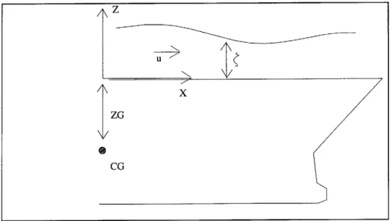
two-dimensional free surface with the geometry illustrated in Figure 4-1. Many of the variables

in the governing equations are not defined in the figure. Of these, ui is the ship surge velocity,

u3 is the ship heave velocity, E is the pitch angle, u5 is the angular velocity, and g is acceleration

due to gravity. Note that u is the water particle velocity in the x-direction. The governing

equations in vector form is

aW a F O H

-+ = [D] + C (4.1)

go _,Ug( 0 0 0

whereW= ,, F= ugH 2 ,g) [D](= qjg(+q2U+q3

ug

u

2

_g+(gC)

2 ₂

and C = . The variables qi through q4 are functions of deck motion and geometry.

(q4g(

They are defined as

U5 2

(34)

z

ZG

CG

Figure 4-1: Coordinate System for Two-Dimensional Free Surface

U5

q2= 2-9 du3 1 q3 = cos(9) dt g du5 X dt g (u5 )2 ZG g fdull\ dU5Z q4 = sin()- d + U + du ZG

Equation 4.1 is derived by applying the shallow water assumptions to the continuity equation

and Eulers equations of motion.

The derivatives of the flux vector F and H can be expressed in terms of W

a F

49X

4W

=[

w

and

o71

(9X -4 = [J2] _Ox (4.2)

where [J1] and [J2] are the Jacobian matrices. The eigenvalues of [Ji] are

A = u

+

V/g9 and A2= U - V

with the eigenvectors

el= _{(1,u+ V)} and e=

(4.3)

(35)

The difference of W and flux vector F are approximated as 2 AW4= Zak ek k=1 2 and AF =

S

Akakek k=1

The right hand side of equation 4.1 equal to zero corresponds to water sloshing for a given

initial water surface profile and the ship stationary. With the right hand side zero, the finite

difference scheme with the split flux difference can be expressed in the following form

( n + _ )(- t (A W W

**+ F* F*(4.6)**

i

AX 3--f i+7 where 1 -4 -4 1 2

F* = -(F j+1 + F ) 2 ak,j+i -1 AkJ+i ekJ+

3

2

k=1 2 22 2-2 k- -4 F( F ₂+Fk1) - _k=1 A e 2ak (4.7) (4.8)

The scheme in equation 4.6 is of the first order.

When the right hand side of equation 4.1 is not equal to zero, difference term and projected into the eigenvector space as follows

-+ 2

RH(= [D H 1

The right hand side flux difference, where the flux difference is

ARHS = RHSAx, is then split

)+ 2 2

ARHS.t %J-L+ and ARHS = E

AH 2=- k1

k=12k=

it is treated as another flux

r( t4.9)

related to equation 4.9 by

Yk,J+ kj eekJ+

where

A

Z

1

-k, T1 = , (AkJ.1 AkJ--I) and A i+ . (A J 1 Ak~j

1

The split flux difference is then included in the finite difference scheme of equation 4.6

W(n+l) - (n) At ( _A _H ₊ ₎ A x J

~

i2 x i T 1 A+ 7h~ (4.10) (4.11) (4.12) (4.5)

(36)

The minus sign in equation 4.12 prior to the RH term is due to the minus sign in equation

4.9. In [28] Steger shows that flux splitting schemes are stable if and only if A - < 1.

Shallow water first-order schemes suffer from numerical dissipation (the shock front will be

smeared). Reference [12] shows how a flux limiter, which is a correction term for the numerical

flux, can be applied to the first order scheme to make the scheme higher order.

The flux difference splitting method can be used to solve the shallow water equations for a

three-dimensional free surface. Reference [12] formulates a technique using the flux difference

splitting method, together with the Fractional Step Method [32], so that solutions to the shallow

water equations can be obtained by solving two sets of two-dimensional free surface problems.

The three-dimensional solution works as follows. Two sets of vector equations similar to

equation 4.1 are devised. One set is for flow in the ship longitudinal direction (x - axis)

where each specific equation holds for a certain deck strip of thickness Ay. The other set of

vector equations is for flow in the transverse direction ( y - axis) where each equation is for a

certain deck strip of thickness Ax. Then the Fractional Step Method advances the solution in

time. At each time step the sets of equations along the x - axis are solved for an intermediate

solution assuming no y dependency. Then, in the same time step, the sets of equations along

the y - axis are solved from the intermediate solution assuming no x dependency. Instead

of solving the three-dimensional free surface governing equation on (m x n) nodes, a total of

(m+n) two-dimensional free surface equations are solved along the x and y directions separately using the Fractional Step Method.

The difference schemes of equations 4.6 and 4.12 for a two-dimensional free surface were

programmed in a computer so that the method could be compared with Glimms method.

4.3 Glimms Method (Random Choice Method) for Water

Mo-tion on Deck

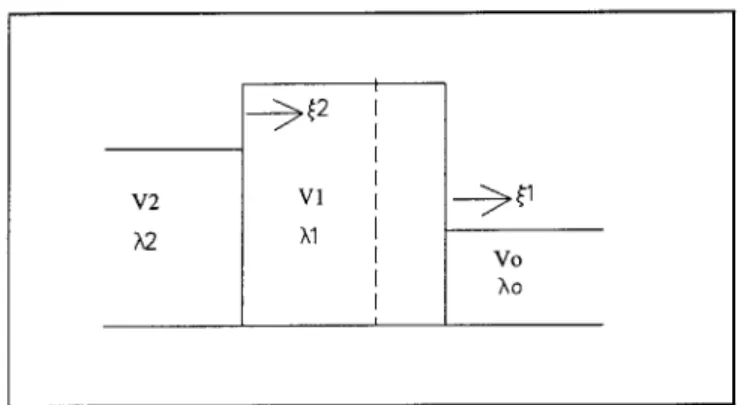
For a two-dimensional free surface, Glimms Method is performed by dividing the physical

domain into intervals, i = 1, 2, 3, ... , i max. In each interval at time nAt the solution is

approxi-mated by piecewise constant depth, (j, and particle velocity, ui. At the boundary between each

Changing mass applications in an advanced time domain ship motion program

Changing Mass Applications in an Advanced Time Domain

Ship Motion Program

by

Paul Richard Wynn

B.S., Virginia Tech (1986)

Submitted to the Department of Ocean Engineering

in partial fulfillment of the requirements for the degree of

Naval Engineer

at the

MASSACHUSETTS INSTITUTE OF TECHNOLOGY

June 2000

o

2000 Paul R. Wynn. All rights reserved.

The author hereby grants to MIT permission to reproduce

and to distribute publicly paper and electronic

copies of this thesis document in whole or in part.

Signature of Author ...

...

Department of Ocean Engineering

22 May 2000

C ertified by ...

...

Dick K.P. Yue

Professor of Hydrodynamics and Ocean Engineering

Thesis Supervisor

A ccepted by ...

...

Nicholas M. Patrikalakis

Kawasaki Professor of Engineering

Changing Mass Applications in an Advanced Time Domain Ship Motion

Program

Abstract

Contents

List of Figures

. . . 77

Chapter 1

Introduction

1.1

Background

1.2

Research Objectives

[7],

[19].

Chapter 2

LAMP Description and

Development of Equations of Motion

2.1

LAMP Description

[211.

Sf

S,

V

t > 0

a5I

at

L

1/IP

Q1.

Q

#D1

at

az

oo

at

+

j

)InGO)dS

{Im(

an

cBn

c8n

Sb,

Sm.

2.2

LAMP Rigid Body Dynamics

E,

E,

O/.

I

_az

_at