Concept Generalization in Visual Representation Learning

HAL Id: hal-03110632

https://hal.inria.fr/hal-03110632

Preprint submitted on 14 Jan 2021

HAL is a multi-disciplinary open access

archive for the deposit and dissemination of

sci-entific research documents, whether they are

pub-lished or not. The documents may come from

teaching and research institutions in France or

abroad, or from public or private research centers.

L’archive ouverte pluridisciplinaire HAL, est

destinée au dépôt et à la diffusion de documents

scientifiques de niveau recherche, publiés ou non,

émanant des établissements d’enseignement et de

recherche français ou étrangers, des laboratoires

publics ou privés.

Concept Generalization in Visual Representation

Learning

Mert Bulent Sariyildiz, Yannis Kalantidis, Diane Larlus, Karteek Alahari

To cite this version:

Mert Bulent Sariyildiz, Yannis Kalantidis, Diane Larlus, Karteek Alahari. Concept Generalization in

Visual Representation Learning. 2020. �hal-03110632�

Concept Generalization in Visual Representation Learning

Mert Bulent Sariyildiz

Yannis Kalantidis

Diane Larlus

Karteek Alahari

1

_{NAVER LABS Europe}

_Inria

Abstract

Measuring concept generalization, i.e., the extent to which models trained on a set of (seen) visual concepts can be used to recognize a new set of (unseen) concepts, is a popular way of evaluating visual representations, es-pecially when they are learned with self-supervised learn-ing. Nonetheless, the choice of which unseen concepts to use is usually made arbitrarily, and independently from the seen concepts used to train representations, thus ignor-ing any semantic relationships between the two. In this paper, we argue that semantic relationships between seen and unseen concepts affect generalization performance and propose ImageNet-CoG, a novel benchmark on the Ima-geNet dataset that enables measuring concept generaliza-tion in a principled way. Our benchmark leverages expert knowledge that comes from WordNet in order to define a sequence of unseen ImageNet concept sets that are seman-tically more and more distant from the ImageNet-1K sub-set, a ubiquitous training set. This allows us to benchmark visual representations learned on ImageNet-1K out-of-the box: we analyse a number of such models from supervised, semi-supervised and self-supervised approaches under the prism of concept generalization, and show how our bench-mark is able to uncover a number of interesting insights. We will provide resources for the benchmark at https: //europe.naverlabs.com/cog-benchmark.

1. Introduction

Supervised learning has been a key factor behind the success of deep neural network-based models for many computer vision problems. However, collecting manually-annotated large-scale data for each problem is not a sus-tainable paradigm. There has been an increasing effort to tackle this issue by learning transferable visual representa-tions across related problems, especially to the ones where annotations are scarce. Prior work has achieved this in var-ious ways; For instance, by imitating knowledge transfer in low-data regimes [16,61], exploiting unlabeled data in a

*_{Univ. Grenoble Alpes, Inria, CNRS, Grenoble INP, LJK, 38000}

Greno-ble, France

L

L

L

L

L

L

Unseen Concepts

(Levels)

Seen Concepts

(from IN-1K)

Semantic

_distance

Full ImageNet Concept Set

Figure 1: ImageNet-CoG is a new benchmark for evaluating the Concept Generalization capabilities of visual representa-tions. In this benchmark, we extract features from models trained on the 1000 seen concepts of the ImageNet ILSVRC dataset [50] (IN-1K) and evaluate them on several concept generalization levelsL1/···/5, each consisting of 1000 unseen concepts sampled from the rest of ImageNet [13]. These lev-els are created so they contain concepts that are semantically less and less similar to IN-1K.

self- [8,20,23] or weakly- [28,37,68] supervised manner. The quality of the learned visual representations for trans-fer learning is usually determined by checking whether they are useful for, i.e., generalize to, a wide range of down-stream vision tasks. Therefore, it is important to quantify this generalization, which has several facets, such as gener-alization to different input distributions (e.g., from synthetic images to natural ones), to new tasks (e.g., from image clas-sification to object detection), or to different semantic con-cepts (e.g., across different object categories or scene labels). Though the first two facets have received much attention recently [19,21], we observe that a more principled analysis is needed for the last one.

As also noted by [14,73], the effectiveness of the knowl-edge transfer between two tasks is closely related to the semantic similarity between the concepts of interest consid-ered in each task. However, assessing this relatedness of tasks is not straightforward, as the semantic extent of a con-cept may depend on the task itself. For instance, in the case of image classification it can be a coarse- or fine-grained object category such as “car” [15] or “Russian blue” [43], as well as a less defined concept such as “dining hall” [76]. Consequently, while testing the transfer learning capabilities of models, exhaustive lists of downstream tasks have been considered to cover wide ranges of concepts [8,30]. Yet, previous attempts discussing this issue have been limited to intuition [48,73]. We still know little about the impact of the semantic relationship between the concepts seen during training visual representations and those seen during their evaluation (seen and unseen concepts, respectively).

In this paper, we propose to study the generalization ca-pabilities of visual representations across concepts that exist in a large, popular and broad ontology, i.e., ImageNet [13], while keeping all other generalization facets fixed. Starting from a set of seen concepts, the popular ILSVRC dataset (IN-1K), we utilize semantic similarity metrics that use the hand-crafted ontology to measure semantic distance between IN-1K and every unseen concept, in order to define a se-quence of five, IN-1K-sized concept generalization levels, each consisting of a distinct set of unseen concepts with in-creasing semantic distance to the seen ones. This results in a large-scale benchmark that consists of thousands of concepts, that we refer to as the ImageNet Concept Generalization benchmark, or ImageNet-CoG in short. Fig.1illustrates the different generalization levels.

We define a set of experiments that allows us to explore a number of important questions. (i) Which methods are more resilient to the semantic distance between seen and unseen concepts, hence generalize better? (ii) How fast can methods learn new concepts? and (iii) What makes them behave in certain ways? Defining our benchmark “around” IN-1K, allows us to fairly compare models trained on IN-1K out-of-the box. Using their publicly available pretrained models, we analyse a number of recent supervised, semi-supervised and self-semi-supervised approaches under the prism of concept generalization, and show how our benchmark is able to uncover a number of interesting insights.

Contributions. First, we propose a systematic way of studying concept generalization, by explicitly defining a set of seen concepts which visual representation learning approaches are exposed to, and unseen concepts which are the ones visual representations need to generalize to dur-ing evaluation. Second, we design a large-scale benchmark, ImageNet-CoG, which embodies this systematic way. It builds on ImageNet and allows for a fine-grained analysis of concept generalization thanks to several increasingly more

challenging evaluation levels. Third, we analyse in depth the generalization behavior of several state-of-the-art visual representation learning approaches on our benchmark.

2. Related Work

Since our work deals with models generalizing to visual concepts beyond the training set, it is related to knowledge transfer methodologies across sets of concepts, as well as practices to evaluate the quality of visual representations. Generalization. It typically refers to the ability of a model to perform well on new data, unavailable during its train-ing phase. It has been studied under different perspectives such as regularization [56] and augmentation [74] tech-niques, links to human cognition [18], or developing quanti-tative metrics to better understand it, e.g., through loss func-tions [34] or complexity measures [42]. Several dimensions of generalization have been explored in the realm of com-puter vision, for instance, generalization to different visual distributions of the same concepts (domain adaptation) [11], or generalization across tasks [75]. Generalization across conceptsis a crucial part of zero- [51,55] and few-shot [61] learning. We also study this particular dimension, i.e., con-cept generalization, where the goal is to transfer knowledge acquired on a set of seen concepts, to newly encountered unseenconcepts as effectively as possible.

Towards a structure of the concept space. One of the first requirements for rigorously evaluating concept generaliza-tion is structuring the concept space, in order to analyze the impact of concepts present during pretraining and transfer stages. However, previous work rarely discusses the par-ticular choices of splits (seen vs. unseen) of their data, and random sampling of concepts remains the most common approach [22,26,32,66]. A handful of methods leverage existing ontologies, for instance the WordNet graph [41] is used as a reference for splitting [12,17,33,73] or domain-specific ontologies are used to test cross-domain generaliza-tion [21,63]. These splits are however based on heuristics, instead of principled mechanisms that take into account the semantic relationship of concepts.

Transfer learning evaluations. While evaluating the qual-ity of visual representations, it has become a standard to benchmark models on various tasks such as classification, detection, segmentation and retrieval [6,8,19,23,30,52,53]. These tasks are generally performed on datasets such as ImageNet-1K [50], Places [76], SUN [67], Pascal-VOC [15], MS-COCO [36]. Such choices, however, are often made independentlyfrom the dataset used to train the visual repre-sentations, ignoring their semantic relationship.

In summary, semantic relations between pretraining and transfer tasks has been overlooked in evaluating the quality of visual representations. To address this issue, we present a controlled evaluation protocol that factors in such relations.

3. The ImageNet Concept Generalization

Benchmark

Our ImageNet-CoG is composed of multiple image sets, one for pretraining and several transfer datasets, curated in a controlled manner to measure the transfer learning per-formance of visual representations. Sec.3.1discusses our motivation for ImageNet-CoG. Sec.3.2presents the pretrain-ing dataset, i.e., the set of concepts seen durpretrain-ing the repre-sentation learning phase. Sec.3.3presents our approach to construct transfer datasets, i.e., sets of unseen concepts or levels of decreasing semantic similarity to the seen ones. Finally, Sec.3.4explains the proposed evaluation protocol for measuring different facets of concept generalization. We present an overview of the benchmark in the gray box.

3.1. Background

Transfer learning performance is highly sensitive to the semantic similarity between concepts in the pretraining and target datasets [14,73]. Studying this relationship requires carefully constructed evaluation protocols controlling (i) which concepts a model has been exposed to during train-ing (i.e., seen concepts), (ii) the semantic distance between these seen concepts and those considered for the transfer task (i.e., unseen concepts). As discussed earlier, state-of-the-art evaluation methods severely fall short on handling these aspects. We present a solution to fill in this gap by proposing ImageNet-CoG.

While designing ImageNet-CoG, we considered several important points. First, in order to exclusively focus on con-cept generalization, we need a controlled setup tailored for this specific aspect of generalization, i.e., we need to make sure that the only thing that changes between the pretraining and the transfer datasets is the set of concepts. In particular, we need to fix the input image distribution (i.e., natural im-ages), and the nature of the annotation process (which may determine the statistics of images [59]).

Second, to better understand the relationship between the semantic similarity of some seen and unseen concepts and the knowledge transfer across them, we need a suffi-ciently broad set of concepts, not specialized fine-grained ones, such as bird species [62]. Moreover, to determine the semantic similarity between two concepts, we need an auxil-iary knowledge base that can provide a notion of semantic relatedness. It can be manually defined (e.g., WordNet [41]), requiring expert knowledge, or automatically constructed, for instance by a language model (e.g., word2vec [40]).

Third, the choice of the pretraining and target datasets is crucial. We need these datasets to have diverse object-level images [3] and to be as less biased as possible, e.g., towards canonical views of concepts [39]. We also need their images to be carefully annotated for computing concept generalization precisely.

The ImageNet-CoG benchmark in a nutshell Prerequisites:

A set of seen concepts

Train/val/test images associated to seen concepts A model pretrained on the seen concepts

Sets of unseen concepts organized in levelsL1/2/3/4/5 Train/val/test images for each levelL1/2/3/4/5 Phase 1: Feature Extraction

Use the model to extract image features for all image sets. Phase 2: Evaluation

Run each experiment for seen concepts and for each level L1/2/3/4/5, separately:

• Learn linear classifiers using all available training data How resilient is my model to the semantic distance be-tween seen and unseen concepts?

• Learn linear classifiers using N _{∈ {1, 2, 4, . . . , 128}} training samples per concept.

How fast can methods adapt to new concepts?

• Apply k-means clustering on all features withk = the number of concepts in each level

How does the embedding space of my model cluster for seen/unseen concepts?

• Compute the alignment and uniformity scores [64] How is the embedding space of my model structured for seen/unseen concepts?

With all these requirements in mind, we could either collect a new dataset or build on top of an existing one. We chose the latter and narrowed our scope to the set of concepts from the full ImageNet dataset [13]. ImageNet contains 14,197,122 curated images covering 21,841 concepts, all of which are further mapped to a hand-crafted ontology [41], allowing us to define reliable semantic similarities.

3.2. Seen concepts

The first step is to select a set of concepts from ImageNet, which will be used to learn visual representations. For this, we make the obvious choice, and define seen concepts as the categories from the ubiquitous ILSVRC 2012 dataset [50] (IN-1K), which is a subset of the full ImageNet [13]. It con-sists of 1.28M images over 1000 concepts and has been used as the standard benchmark for evaluating novel CNN archi-tectures (backbones) as well as self- and semi-supervised models [7,9,20,23,64,69].

Choosing IN-1K as the seen classes further offers sev-eral advantages that make our benchmark easily applicable. (i) Practitioners would train their models on IN-1K, as this is standard practice; then they can simply evaluate on our benchmark with their pretrained models. (ii) It enables us to benchmark visual representations learned on IN-1K

out-... ... ... ... ... ... The pool of 5754 unseen concepts from the full ImageNet (excluding IN-1K): (i) with at least 782 images, (ii) not in the "person" sub-tree, and (iii) leaf nodes

... ... ...

Figure 2: Sampling of unseen concepts for each level. We rank the 5754 eligible unseen concepts with respect to their semantic similarity to the IN-1K set using Eq. (2), and depict them ranked in this figure in decreasing similarity (from left to right). We then sample 5 groups of 1000 concepts each such that the entire range of similarities is captured. Gray-shaded areas correspond to concepts that are ignored.

-of-the box, by using the publicly available checkpoints of the models (as shown in Sec.4).

3.3. Concept generalization levels

Our next step is defining a sequence of unseen concept sets, each with decreasing semantic similarity to the seen concepts. These datasets of unseen concepts, or levels, would allow to measure concept generalization in a controlled set-ting. Having decided on the seen dataset as IN-1K, next, we sample unseen datasets from the extended ImageNet [13] dataset, such that they are determined by their semantic sim-ilarityto IN-1K. We specifically use the Fall 2011 snapshot of ImageNet, that contains 21,841 concepts, including the ones in IN-1K. We perform this sampling in a controlled manner to obtain multiple unseen datasets that are increas-ingly less similar semantically to IN-1K. We thus create increasingly difficult transfer learning scenarios from the seen to the unseen concepts.

Design choices for concept generalization levels. We de-sign our concept generalization levels to be as comparable as possible to IN-1K. Following [50], we select concepts with a minimum of 732 and a maximum of 1300 training images, plus 50 images for testing. As it was recently shown that a subset of ImageNet categories might exhibit problematic behavior in downstream computer vision applications [72], we make sure that no concept under the “person” sub-tree is selected. We further make sure that each level contains only leaf nodes, i.e.,c1is not a child or parent ofc2, for anyc1 andc2 in any level. These requirements limit the set of eligible unseen ImageNet concepts from 20,841 to 5754, from which we chose 5 levels of 1000 concepts each, sampled to maximize their diversity with respect to IN-1K (details on the sampling process are presented below). This brings the total number of training images per level to 1.10 million, which is close to 1.28 million training images of IN-1K.

Semantic similarity between concepts. Computing the se-mantic similarity of any two concepts requires defining each concept in a semantic knowledge base. Fortunately,

Im-ageNet is built onto the word ontology of WordNet [41], where synonyms of words corresponding to distinct con-cepts are grouped into “synsets,” which are linked according to their semantic relationships. This further allows to utilize existing semantic similarity measures [5] that exploit the graph structure of WordNet to capture the semantic related-ness of pairs of concepts. We use the Lin similarity [35] to define concept-to-concept similarities. This similarity of two conceptsc1andc2is given by:

simLin(c1, c2) = 2× IC(LCS(c1, c2))

IC(c1) + IC(c2) , (1) where LCS denotes the lowest common subsumer of two concepts in the WordNet graph, and IC(c) =_{− log p(c) is} the information content of a concept withp(c) being the probability of encountering an instance of the concept c in a specific corpus (in our case the subgraph of WordNet including all the seen and unseen concepts and their parents till the root node). Following [49], we definep(c) as the number of concepts that exist underc.

Semantic similarity between levels. We extend the notion of concept-to-concept similarity to sets of concepts in order to define similarities between the set of seen (IN-1K) and each unseen concept. This asymmetric similarity between the set of seen concepts_CIN-1Kand any unseen conceptc is given by:

simIN-1K(c) = max(_{simLin(c, ˜c)_{| ˜c ∈ C}IN-1K}), (2) i.e., as the maximum similarity between any concept from IN-1K andc. Using Eq. (2), we rank all unseen concepts with respect to their similarity to IN-1K and sample 5 sets of 1000 concepts as shown in Fig.2. This selection process creates challenging levels (the 1000 concepts within a level are as similar as possible to each other) which span over the full set (the margin between levels is constant and as large as possible). As a result, we maximize the range of the unseen concepts with respect to their semantic similarity to the seen ones.

Other semantic similarity measures. While designing our benchmark, we considered different semantic similarity mea-sures before choosing Lin similarity. We explored other measures defined on the WordNet graph [38], such as the path-based Wu-Palmer [65] and the information content-based Jiang-Conrath [27]. We also considered semantic similarities based on Word2Vec representations [40] of the titles and textual descriptions of the concepts. However, our initial experiments show that benchmarks built using differ-ent similarity measures led to the same main observations we present in Sec.4. For more details, see the supplementary material for additional results with an alternative benchmark constructed using Word2Vec.

3.4. Proposed evaluation protocol

We now present the evaluation protocol for ImageNet-CoG, and summarize the metrics we report for the different experiments presented in Sec.4.

Feature extraction and pre-processing. We base our pro-tocol on the assumption that good visual representations should generalize to new tasks with minimal effort, i.e., with-out fine-tuning the backbones. Therefore, for our benchmark, we only use the pretrained backbones as feature extractors and decouple representation from our evaluation. Concretely, we assume a model learnt on the training set of IN-1K; we use this model as an encoder to extract features, for IN-1K and all the five levelsL1/2/3/4/5.

Recent findings [29] suggest that residual connections prevent backbones from overfitting to pretraining tasks and the features extracted from the last layer of ResNet-like ar-chitectures generalize better to transfer tasks. In light of this, we perform all our evaluations on the features x_{∈ R}2048 extracted from the global average pooling layer of the pre-trained ResNet50 backbones. Moreover, in our evaluations no fine-tuning or data-augmentation is applied.

Finally, we observed that the`2-norms of features from different models vary significantly across sets. To elimi-nate any bias towards the magnitudes of the features, unless otherwise stated, we`2-normalize them.

Train/val/test splits. We randomly select 50 samples as the test set for each concept and use the remaining ones (at least 732, at most 1300) as a training set. For evaluations that involve hyperparameters, we randomly sample20% of the training sets to choose the hyperparameters (see below). We report results only on the test sets.

Setting hyperparameters. To train linear classifiers in a fair manner for all models, we choose the learning rate and weight decay parameters on the validation sets by using Op-tuna [1] (for each level and IN-1K,20% of its training set is randomly sampled as its validation set). Once we set the hyper-parameters, we train the final classifiers using the train-ing and validation sets and compute the final performance on the test sets. We repeat the hyper-parameter selection 5 times with different seeds, and report the mean of the final scores (in most cases, standard deviation is_{≤ 0.2, and is not} visible in figures).

Learning linear classifiers. We train a linear logistic re-gression model (LogReg) on each level. In each LogReg, we compute class logits simply as s = Wx + b, where W_{∈ R}1000×2048and b_{∈ R}1000are the parameters to learn. We use all the training samples (N = All) available for each concept.

Learning from few samples per concept. We also propose to evaluate data efficiency of models in learning unseen con-cepts, by performing few-shot concept classification on each level. We argue that this aspect of concept generalization is

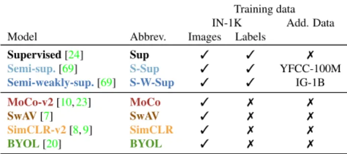
Table 1: Benchmarked models and their training data. We use the best officially-released ResNet-50 checkpoints for each model. For Sup, we use the pretrained ResNet-50 model available in the torchvision package of pytorch [44]. “Add. Data” refers to the additional data used for pretraining.

Model Abbrev.

Training data

IN-1K Add. Data

Images Labels

Supervised [24] Sup 3 3 7

Semi-sup.[69] S-Sup 3 3 YFCC-100M Semi-weakly-sup.[69] S-W-Sup 3 3 IG-1B

MoCo-v2[10,23] MoCo 3 7 7

SwAV[7] SwAV 3 7 7

SimCLR-v2[8,9] SimCLR 3 7 7

BYOL[20] BYOL 3 7 7

particularly important as it assesses the ability of models to adapt to unseen concepts, with only a small number of anno-tated samples. We follow the same LogReg setup described above, except that we train LogRegs with a few samples per concept, i.e.,N _{∈ {1, 2, 4, 8, 16, 32, 64, 128}.}

Clustering experiments. We performk-Means clustering and learn1000 cluster centroids (as many as the concepts in each level) on the training sets. We use the cuMLk-Means implementation [47], repeat clustering with 3 seeds and com-pute cluster assignments for test samples using the centroids that gave the lowest inertia across the 3 runs. We report clus-tering metrics, including cluster purity and adjusted [60] and normalized mutual information scores between the cluster assignments and the labels of the test samples.

Alignment and uniformity. We compute alignment and uniformity scores, as presented in [64], using the test sets from each level and from IN-1K.

4. Evaluating state-of-the-art models

We now analyse how state-of-the-art models behave on our ImageNet-CoG, i.e., on increasingly difficult concept generalization levels. For clarity, we show in this section a subset of our experiments, which lead to the most inter-esting conclusions. We provide additional analyses in the supplementary material, together with details regarding implementation.

4.1. Models

We select a diverse set of models pretrained on IN-1K to analyse; a summary is shown in Tab.1. We first con-sider three models that use the ground-truth labels of IN-1K directly. Sup refers to a model trained in the com-mon supervised setting [24], whileS-Sup and S-W-Sup are the semi-supervised and semi-weakly-supervised mod-els from [69], respectively. They are pretrained on YFCC-100M [58] and IG-1B [37] and then fine-tuned on IN-1K.

Sup S-Sup S-W-Sup MoCo SimCLR SwAV BYOL IN-1K L1 L2 L3 L4 L5 50 60 70 80 T op-1 accurac y (a) IN-1K L1 L2 L3 L4 L5 −6 −4 −2 0 2 4 6 T op-1 accurac y relati v e to Sup (b) IN-1K L1 L2 L3 L4 L5 −30 −20 −10 0 T op-1 accurac y dr op w .r .t. IN-1K (c)

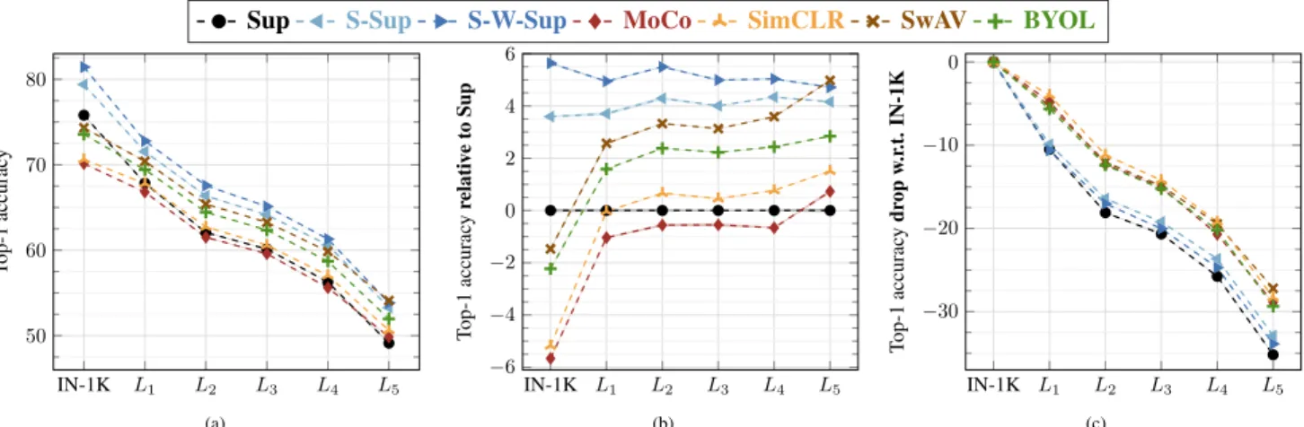
Figure 3: Top-1 accuracy for each method (pretrained on IN-1K) using logistic regression classifiers. We train them on pre-extracted features for the concepts in IN-1K or in one of our generalization levels (L1/2/3/4/5), with all the training samples, i.e., N= All. (a)-(c) are visualizations of the same results from different perspectives. (a), (b) and (c) show the absolute top-1 accuracy, performance relative to Sup, and the drop in performance on the levels relative to IN-1K, respectively.

Finally, given the outstanding transfer learning performance that contrastive self-supervised approaches have recently exhibited, we benchmark four of the best performing ones: BYOL[20],MoCo[10,23],SimCLR[8,9] andSwAV[7].

MoCoandSimCLRshare many similarities: they both train with a contrastive loss where positive pairs are obtained by applying heavy transformations to an image, with all the other images being treated as negatives. The main difference lies on the momentum encoder used byMoCoto sample a negative, while for SimCLR negatives come from the images of the same mini-batch. BYOLis similar to this, except that it does not require negative samples.SwAVis a hybrid approach which combines contrastive training with a clustering approach. It enforces consistency between the cluster assignments produced by different augmentations, and further appends a new data augmentation strategy that uses a mix of views with different resolutions. For each model, we use the best ResNet-50 [24] backbone released by their authors. As it is not clear if YFCC-100M or IG-1B contain images of our unseen concepts, these two models are not directly comparable to the others.

4.2. Generalization to unseen concepts

First, we conduct transfer learning experiments on sets of unseen concepts at different concept generalization lev-els. Specifically, we perform concept classification on each level separately, and study (i) how classification performance changes as we semantically move away from the seen con-cepts, and (ii) how fast can models adapt to unseen concepts. Generalization using linear classifiers. We present the results in Fig.3and highlight the following observations.

(a) Performance of all the models (Fig.3a) monotonically decreases as we move from levels with concepts semantically

closer to the seen ones, to those further away. This seemingly obvious observation grounds the remainder of our study.

(b) Focusing on the supervised methods, we note that the rankingS-W-Sup>S-Sup> Sup remains consistent across levels. In fact, from Fig.3b, we see that the gains ofS-W-SupandS-Supover Sup remain almost constant. This shows that pretraining with additional data on IG-1B or YFCC-100M helps in generalizing better, even for seman-tically distant concepts. It is also noteworthy that, as we go from IN-1K toL5, the difference betweenS-W-Supand S-Sup, despite the former utilizing an order of magnitude more data, reduces from2% to 0.5%.

(c) Interestingly, despite the superiority of Sup over the self-supervised models when evaluated on IN-1K, it is out-performed byBYOLandSwAVconsistently on all the un-seen levels, by significant margins (see Fig. 3b). We hy-pothesize that by learning augmentation invariance in a soft way (BYOLhas practically no negatives, whileSwAVonly enforces “soft” consistency through the cluster assignments of different augmentations) these two approaches produce representations that generalize better.

(d) We also note that from IN-1K to L5 performance gaps between Sup and the self-supervised models progres-sively shift in favor of the self-supervised models. This leads to0.8%, 5.0%, 1.5% and 2.9% margins achieved by

MoCo,SwAV,SimCLRand BYOL, respectively, onL5 (see Fig.3b). Since these self-supervised methods essen-tially learn from data augmentation, it implies that learning augmentation invariances transfers better to images of un-seen concepts. This is in line with the observation that data augmentation strategies can significantly boost supervised learning performance as well [74].

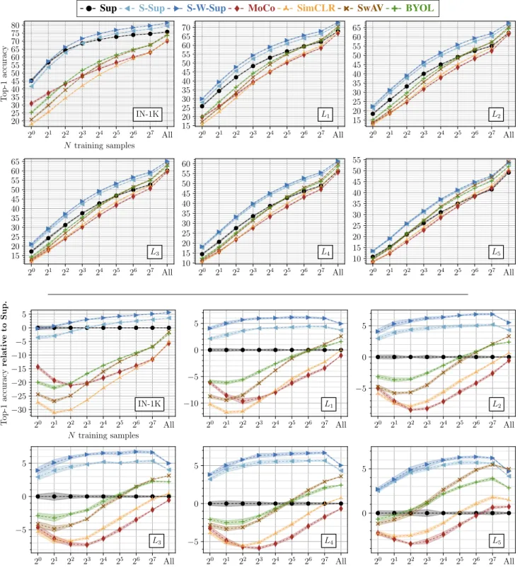
Sup S-Sup S-W-Sup MoCo SimCLR SwAV BYOL 1 2 4 8 16 32 64 128 All 20 30 40 50 60 70 80 IN-1K T op-1 accurac y 1 2 4 8 16 32 64 128 All 20 30 40 50 60 70 _L 1 1 2 4 8 16 32 64 128 All 10 20 30 40 50 L5

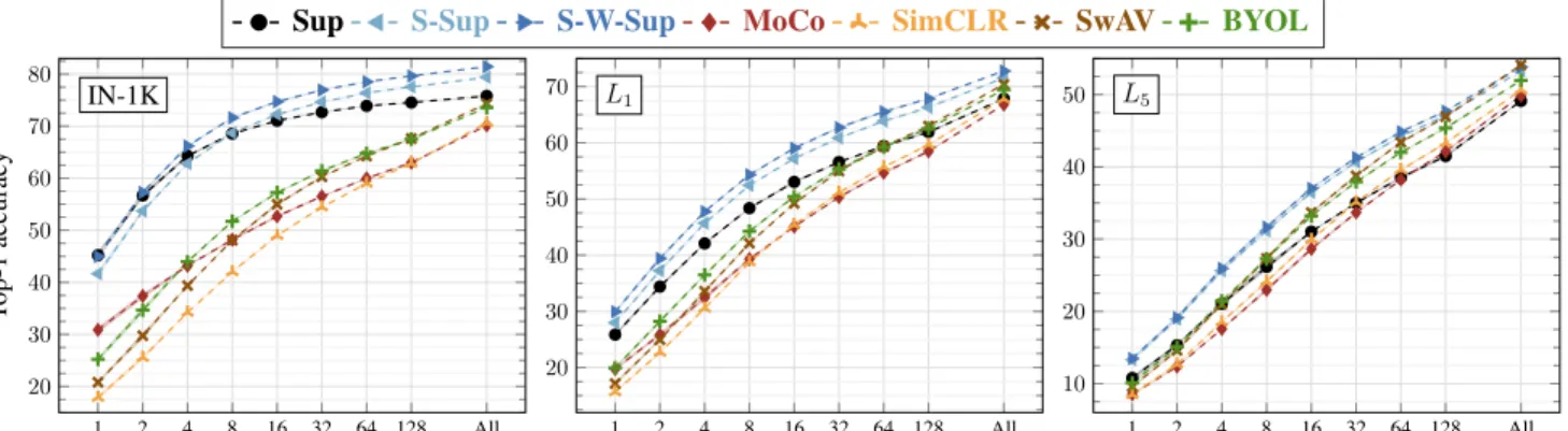
Figure 4: Top-1 accuracy for each method (pretrained on IN-1K) using logistic regression classifiers. We train them on pre-extracted features for the concepts in IN-1K and our generalization levels (L1/2/3/4/5), with a few training samples per concept, i.e.,N =_{{1, 2, 4, 8, 16, 32, 64, 128}. “All,” the performance when all the samples are used, is also shown for} reference. From left to right: results obtained on IN-1K,L1, andL5. (See the supplementary material for the remaining levels.)

the other self-supervised approaches on all levels. Starting fromL1, it even outperforms Sup by an increasing margin as the unseen concepts become semantically less similar. More surprisingly, SwAVoutperformsS-Supand S-W-Supby 0.8% and 0.3% on L5, showing strong generalization ability. We believe that the hybrid nature ofSwAVgives it an edge compared to other self-supervised approaches which only focus on instance discrimination, while the extra inter-scale augmentation may further provideSwAVwith an invariance that assists generalization.

(f) Finally, from Fig.3cwe observe the difficulty in gener-alizing to semantically dissimilar concepts. All the methods, evenS-W-Suppretrained on 1 billion images, lose25_−35% of their classification power, relative to their performance on the seen classes.

Generalization from a few samples per concept. Next, we evaluate how fast each model can be trained to classify new concepts by performing few-shot image classification, and the impact of the semantic distance between unseen and seen concepts. We present these results in Fig.4, and make the following observations.

(a) Sup is significantly and consistently better at learning in low-data regimes, i.e., N = _{{1, 2, 4, 8}, on L}1/2/3/4. However, onL5, the best performing self-supervised model (BYOLorSwAV) is on par or better than Sup for allN .

(b) As we go from IN-1K to L5, the amount of an-notated data required for the self-supervised models to match the supervised ones decreases consistently. For instance, SwAV matches the performance of Sup when N = 128, 64, 32, 16, 4 on L1/2/3/4/5, respectively.

(c) Despite the intrinsic similarity betweenMoCoand SimCLR,MoCoperforms significantly better whenN = {1, 2, 4, 8} on IN-1K and L1. This is likely due to the mem-ory inMoCoproviding a diverse set of images from (possi-bly) all IN-1K concepts at every step during the pretraining

phase, therefore better approximating a 1-vs-all classification problem for each query. This wayMoCocan learn better class representatives for the concepts in IN-1K and also for the ones semantically close to IN-1K.

(d)BYOLconsistently improves overSwAVon IN-1K and L1,2,3 for smaller numbers of training samples, but SwAV matches or outperforms BYOL provided enough data.

4.3. Topology of the feature space across levels

4.3.1 Clustering of concepts

We expect each model, constructed with either supervised or self-supervised objectives, to learn a feature space where the images of the same concepts are (naturally) clustered. We investigate to what extent this occurs for unseen concepts.

To this end, we performk-Means clustering and learn 1000 cluster centroids (the number of concepts in each level) on the training sets of each level. We then compute cluster purity scores between the cluster assignments and the labels of the test samples. Higher scores here imply that the features are better clustered.

Results. In Fig.5we plot cluster purity across levels. The results presented in this figure are consistent under differ-ent evaluation measures we explored, e.g., rand-index [46], normalized or adjusted [60] mutual information (see the sup-plementary material for details). We observe the following.

(a) The supervised models are significantly better than the self-supervised ones on IN-1K and all the levels. However, BYOLandSwAVreduce the gap with Sup onL5.

IN-1K L1 L2 L3 L4 L5 0.2 0.3 0.4 0.5 0.6 Cluster purity Sup S-Sup S-W-Sup MoCo SwAV SimCLR BYOL

Figure 5: Cluster purity scores between the cluster assign-ments predicted byk-Means and the concept labels, com-puted on the test set of each level.

IN-1K L1 L2 L3 L4 L5 0 −2 −4 −6 ·10−2 Sup S-Sup S-W-Sup MoCo SwAV SimCLR BYOL

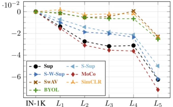
Figure 6: Alignment over uniformity ratio relative to IN-1K computed on the test set of each level.

(b) It is interesting thatMoCois the best self-supervised model on IN-1K and shares the lead withBYOLonL1.

(c)BYOLoutperformsSwAVconsistently on all levels. This observation seems to contradict the performance gains forSwAVoverBYOL across the levels for linear classi-fication. However, we see that the features ofBYOLare more spread over the hyper-spheres compared toSwAV(see Sec.4.3.2and the supplementary material regarding unifor-mity analysis). ForBYOL, this may suggest that although the concepts are less linearly separable, since its features are distributed more uniformly on the hyper-sphere, more natural clusters of concepts appear in its feature spaces. 4.3.2 Measuring alignment and uniformity

In our final evaluation, we visit the recently proposed align-ment and uniformity measures [64], which are powerful tools to better understand the topology of a feature space. Essen-tially, alignment evaluates the compactness of the classes, whereas uniformity measures how spread the samples are regardless of their class label (see [64] for further details on

these scores).

Using the test sets for each level, we compute the align-ment and uniformity scores separately, and for brevity, in Fig.6we report the ratio of alignment over uniformity scores, computed relative to IN-1K. See the supplementary material for more results.

Results. We make the following observations.

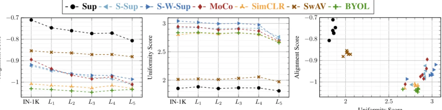
(a) ForSimCLR,SwAVandBYOL, alignment is less af-fected across the levels, and the scores seem to drop slightly only onL5. This is an interesting observation, suggesting that for those methods the features from the same concept are as tightly connected for the seen concepts as they are for the unseen ones.

(b) The behavior noted above does not hold for the rest of the methods, i.e.,MoCo, Sup,S-SupandS-W-Supare highly affected and result in progressively less and less “tight” concept regions fromL1onward.

(c) In terms of uniformity (see supplementary materials for plots), we observe that Sup has the lowest scores ranging from(1.8− 1.9) across all five levels and the seen classes, followed bySwAVranging from(1.9− 2.1), while all the rest of the self-supervised methods, together with the semi-supervised ones were in the(2.6_{− 3.1) range across the six} sets of concepts. In terms of uniformity difference relative to IN-1K,S-W-SupandMoCowere the methods with the highest uniformity score drop onL5.

5. Conclusions and main observations

We introduce ImageNet-CoG, a benchmark for evaluat-ing concept generalization, i.e., the extent to which models trained on a set of seen visual concepts can easily be adapted to recognize a new set of unseen concepts. The seen con-cepts in our benchmark are defined by ImageNet-1K classes, and we built the unseen ones from the full ImageNet dataset and its concept ontology. They organize in levels which are increasingly challenging in terms of concept generalization.

We present extensive evaluations of recent state-of-the-art representation learning models on ImageNet-CoG and make interesting observations: (a) self-supervised models improve their supervised counterpart on unseen concepts, and even challenge semi-supervised ones pretrained with much more data, (b) supervised models are still better at learning in extreme low-data regimes, and (c) different self-supervised methods utilize their feature spaces in different ways.

Our benchmark is designed in a way that it can be used out-of-the-box for IN-1K pretrained models, by extracting features, and performing several experiments with them, on unseen and seen concepts. We envision ImageNet-CoG to be an easy-to-use evaluation suite to study one of the most important aspects of generalization in a controlled and principled way. We plan to make the benchmark public, with extensive documentation and scripts that would enable practitioners to quickly test their models.

Acknowledgements. This work was supported in part by MIAI@Grenoble Alpes (ANR-19-P3IA-0003), and the ANR grant AVENUE (ANR-18-CE23-0011).

References

[1] Takuya Akiba, Shotaro Sano, Toshihiko Yanase, Takeru Ohta, and Masanori Koyama. Optuna: A next-generation hyperpa-rameter optimization framework. In Proc. ICKDDM, 2019. 5,12

[2] Philip Bachman, R Devon Hjelm, and William Buchwalter. Learning representations by maximizing mutual information across views. In Proc. NeurIPS, 2019.14

[3] T. L. Berg and A. C. Berg. Finding iconic images. In Proc. CVPRW, 2009.3

[4] James S Bergstra, R´emi Bardenet, Yoshua Bengio, and Bal´azs K´egl. Algorithms for hyper-parameter optimization. In Proc. NeurIPS, 2011.12

[5] Alexander Budanitsky and Graeme Hirst. Evaluating wordnet-based measures of lexical semantic relatedness. CL, 32(1), 2006.4

[6] Mathilde Caron, Piotr Bojanowski, Julien Mairal, and Ar-mand Joulin. Unsupervised Pre-Training of Image Features on Non-Curated Data. In Proc. ICCV, 2019.2

[7] Mathilde Caron, Ishan Misra, Julien Mairal, Priya Goyal, Piotr Bojanowski, and Armand Joulin. Unsupervised learning of visual features by contrasting cluster assignments. In Proc. NeurIPS, 2020.3,5,6

[8] Ting Chen, Simon Kornblith, Mohammad Norouzi, and Geof-frey Hinton. A simple framework for contrastive learning of visual representations. In Proc. ICML, 2020.1,2,5,6,14 [9] Ting Chen, Simon Kornblith, Kevin Swersky, Mohammad

Norouzi, and Geoffrey Hinton. Big self-supervised models are strong semi-supervised learners. In Proc. NeurIPS, 2020. 3,5,6,14

[10] Xinlei Chen, Haoqi Fan, Ross Girshick, and Kaiming He. Im-proved baselines with momentum contrastive learning. arXiv preprint arXiv:2003.04297, 2020.5,6,14

[11] Gabriela Csurka, editor. Domain Adaptation in Computer Vi-sion Applications. Advances in Computer ViVi-sion and Pattern Recognition. Springer, 2017.2

[12] Jia Deng, Nan Ding, Yangqing Jia, Andrea Frome, Kevin Murphy, Samy Bengio, Yuan Li, Hartmut Neven, and Hartwig Adam. Large-scale object classification using label relation graphs. In Proc. ECCV, 2014.2

[13] J. Deng, W. Dong, R. Socher, L.-J. Li, K. Li, and L. Fei-Fei. ImageNet: A Large-Scale Hierarchical Image Database. In Proc. CVPR, 2009.1,2,3,4,16

[14] Thomas Deselaers and Vittorio Ferrari. Visual and semantic similarity in imagenet. In Proc. CVPR, 2011.2,3

[15] M. Everingham, L. Van Gool, C. K. I. Williams, J. Winn, and A. Zisserman. The PASCAL Visual Object Classes Challenge 2007 (VOC2007) Results.2

[16] Chelsea Finn, Pieter Abbeel, and Sergey Levine. Model-agnostic meta-learning for fast adaptation of deep networks. In Proc. ICML, 2017.1

[17] Andrea Frome, Greg S Corrado, Jon Shlens, Samy Bengio, Jeff Dean, Marc’Aurelio Ranzato, and Tomas Mikolov. De-vise: A deep visual-semantic embedding model. In Proc. NeurIPS, 2013.2

[18] Robert Geirhos, Carlos RM Temme, Jonas Rauber, Heiko H Sch¨utt, Matthias Bethge, and Felix A Wichmann. Generalisa-tion in humans and deep neural networks. In Proc. NeurIPS, 2018.2

[19] Priya Goyal, Dhruv Mahajan, Abhinav Gupta, and Ishan Misra. Scaling and benchmarking self-supervised visual rep-resentation learning. In Proc. ICCV, 2019.1,2

[20] Jean-Bastien Grill, Florian Strub, Florent Altch´e, Corentin Tallec, Pierre H Richemond, Elena Buchatskaya, Carl Do-ersch, Bernardo Avila Pires, Zhaohan Daniel Guo, Moham-mad Gheshlaghi Azar, et al. Bootstrap your own latent: A new approach to self-supervised learning. In Proc. NeurIPS, 2020.1,3,5,6,14

[21] Yunhui Guo, Noel CF Codella, Leonid Karlinsky, John R Smith, Tajana Rosing, and Rogerio Feris. A new benchmark for evaluation of cross-domain few-shot learning. In Proc. ECCV, 2020.1,2

[22] Bharath Hariharan and Ross Girshick. Low-shot visual recog-nition by shrinking and hallucinating features. In Proc. ICCV, 2017.2

[23] Kaiming He, Haoqi Fan, Yuxin Wu, Saining Xie, and Ross Girshick. Momentum contrast for unsupervised visual repre-sentation learning. In Proc. CVPR, 2020.1,2,3,5,6 [24] Kaiming He, Xiangyu Zhang, Shaoqing Ren, and Jian Sun.

Deep residual learning for image recognition. In Proc. CVPR, 2016.5,6,12,18

[25] Sergey Ioffe and Christian Szegedy. Batch normalization: Accelerating deep network training by reducing internal co-variate shift. In Proc. ICML, 2015.18

[26] Dinesh Jayaraman and Kristen Grauman. Zero-shot recog-nition with unreliable attributes. In Proc. NeurIPS, 2014. 2

[27] Jay J Jiang and David W Conrath. Semantic similarity based on corpus statistics and lexical taxonomy. Proc. ICRCL, 1997. 4

[28] Armand Joulin, Laurens van der Maaten, Allan Jabri, and Nicolas Vasilache. Learning visual features from large weakly supervised data. In Proc. ECCV, 2016.1

[29] Alexander Kolesnikov, Xiaohua Zhai, and Lucas Beyer. Re-visiting Self-Supervised Visual Representation Learning. In Proc. CVPR, 2019.5

[30] Simon Kornblith, Jonathon Shlens, and Quoc V. Le. Do better imagenet models transfer better? In Proc. CVPR, 2019.2 [31] Alex Krizhevsky, Ilya Sutskever, and Geoffrey E Hinton.

Im-agenet classification with deep convolutional neural networks. In Proc. NeurIPS, 2012.12,18

[32] C. H. Lampert, H. Nickisch, and S. Harmeling. Learning to detect unseen object classes by between-class attribute transfer. In Proc. CVPR, 2009.2

[33] Chung-Wei Lee, Wei Fang, Chih-Kuan Yeh, and Yu-Chiang Frank Wang. Multi-label zero-shot learning with structured knowledge graphs. In Proc. CVPR, 2018.2

[34] Hao Li, Zheng Xu, Gavin Taylor, Christoph Studer, and Tom Goldstein. Visualizing the loss landscape of neural nets. In Proc. NeurIPS, 2018.2

[35] Dekang Lin. An information-theoretic definition of similarity. In Proc. ICML, 1998.4,16,17,18

[36] Tsung-Yi Lin, Michael Maire, Serge Belongie, James Hays, Pietro Perona, Deva Ramanan, Piotr Doll´ar, and C Lawrence Zitnick. Microsoft COCO: common objects in context. In Proc. ECCV, 2014.2

[37] Dhruv Mahajan, Ross Girshick, Vignesh Ramanathan, Kaim-ing He, Manohar Paluri, Yixuan Li, Ashwin Bharambe, and Laurens van der Maaten. Exploring the limits of weakly supervised pretraining. In Proc. ECCV, 2018.1,5

[38] Lingling Meng, Runqing Huang, and Junzhong Gu. A review of semantic similarity measures in wordnet. IJHIT, 6(1), 2013. 4

[39] Elad Mezuman and Yair Weiss. Learning about canonical views from internet image collections. In Proc. NeurIPS, 2012.3

[40] Tomas Mikolov, Ilya Sutskever, Kai Chen, Greg S Corrado, and Jeff Dean. Distributed representations of words and phrases and their compositionality. In Proc. NeurIPS, 2013. 3,4,16

[41] George A Miller. Wordnet: a lexical database for english. Commun. ACM, 38(11), 1995.2,3,4,16,17,18

[42] Behnam Neyshabur, Srinadh Bhojanapalli, David Mcallester, and Nati Srebro. Exploring generalization in deep learning. In Proc. NeurIPS, 2017.2

[43] Omkar M. Parkhi, Andrea Vedaldi, Andrew Zisserman, and C. V. Jawahar. Cats and dogs. In Proc. CVPR, 2012.2 [44] Adam Paszke, Sam Gross, Francisco Massa, Adam Lerer,

James Bradbury, Gregory Chanan, Trevor Killeen, Zeming Lin, Natalia Gimelshein, Luca Antiga, Alban Desmaison, An-dreas Kopf, Edward Yang, Zachary DeVito, Martin Raison, Alykhan Tejani, Sasank Chilamkurthy, Benoit Steiner, Lu Fang, Junjie Bai, and Soumith Chintala. PyTorch: An imper-ative style, high-performance deep learning library. In Proc. NeurIPS. 2019.5

[45] Fabian Pedregosa, Ga¨el Varoquaux, Alexandre Gramfort, Vin-cent Michel, Bertrand Thirion, Olivier Grisel, Mathieu Blon-del, Peter Prettenhofer, Ron Weiss, Vincent Dubourg, et al. Scikit-learn: Machine learning in Python. JMLR, 12, 2011. 12,16

[46] William M Rand. Objective criteria for the evaluation of clustering methods. JASA, 66(336), 1971.7,16

[47] Sebastian Raschka, Joshua Patterson, and Corey Nolet. Ma-chine learning in python: Main developments and technology trends in data science, machine learning, and artificial intelli-gence. arXiv preprint arXiv:2002.04803, 2020.5

[48] Mengye Ren, Eleni Triantafillou, Sachin Ravi, Jake Snell, Kevin Swersky, Joshua B Tenenbaum, Hugo Larochelle, and Richard S Zemel. Meta-learning for semi-supervised few-shot classification. In Proc. ICLR, 2018.2

[49] Marcus Rohrbach, Michael Stark, and Bernt Schiele. Evaluat-ing knowledge transfer and zero-shot learnEvaluat-ing in a large-scale setting. In Proc. CVPR, 2011.4

[50] Olga Russakovsky, Jia Deng, Hao Su, Jonathan Krause, San-jeev Satheesh, Sean Ma, Zhiheng Huang, Andrej Karpathy, Aditya Khosla, Michael Bernstein, Alexander C. Berg, and Li Fei-Fei. ImageNet Large Scale Visual Recognition Challenge. IJCV, 115(3), 2015.1,2,3,4,11,23

[51] Mert Bulent Sariyildiz and Ramazan Gokberk Cinbis. Gradi-ent matching generative networks for zero-shot learning. In Proc. CVPR, 2019.2

[52] Mert Bulent Sariyildiz, Julien Perez, and Diane Larlus. Learn-ing visual representations with caption annotations. In Proc. ECCV, 2020.2

[53] Ali Sharif Razavian, Hossein Azizpour, Josephine Sullivan, and Stefan Carlsson. Cnn features off-the-shelf: An astound-ing baseline for recognition. In Proc. CVPRW, 2014.2 [54] Karen Simonyan and Andrew Zisserman. Very deep

convo-lutional networks for large-scale image recognition. In Proc. ICLR, 2015.12,18

[55] Richard Socher, Milind Ganjoo, Christopher D Manning, and Andrew Ng. Zero-shot learning through cross-modal transfer. In Proc. NeurIPS, 2013.2

[56] Nitish Srivastava, Geoffrey Hinton, Alex Krizhevsky, Ilya Sutskever, and Ruslan Salakhutdinov. Dropout: A simple way to prevent neural networks from overfitting. JMLR, 15(1), 2014.2

[57] Christian Szegedy, Vincent Vanhoucke, Sergey Ioffe, Jon Shlens, and Zbigniew Wojna. Rethinking the inception ar-chitecture for computer vision. In Proc. CVPR, 2016. 12, 18

[58] Bart Thomee, David A Shamma, Gerald Friedland, Benjamin Elizalde, Karl Ni, Douglas Poland, Damian Borth, and Li-Jia Li. Yfcc100m: The new data in multimedia research. Communications of the ACM, 59(2):64–73, 2016.5 [59] Antonio Torralba and Alexei A Efros. Unbiased look at

dataset bias. In Proc. CVPR, 2011.3

[60] Nguyen Xuan Vinh, Julien Epps, and James Bailey. Informa-tion theoretic measures for clusterings comparison: Variants, properties, normalization and correction for chance. JMLR, 11, 2010.5,7,16

[61] Oriol Vinyals, Charles Blundell, Timothy Lillicrap, Daan Wierstra, et al. Matching networks for one shot learning. In Proc. NeurIPS, 2016.1,2

[62] C. Wah, S. Branson, P. Welinder, P. Perona, and S. Belongie. The Caltech-UCSD Birds-200-2011 Dataset. Technical Re-port CNS-TR-2011-001, California Institute of Technology, 2011.3

[63] Bram Wallace and Bharath Hariharan. Extending and analyz-ing self-supervised learnanalyz-ing across domains. In Proc. ECCV, 2020.2

[64] Tongzhou Wang and Phillip Isola. Understanding contrastive representation learning through alignment and uniformity on the hypersphere. In Proc. ICML, 2020.3,5,8,16

[65] Zhibiao Wu and Martha Palmer. Verb semantics and lexical selection. ACL, 1994.4

[66] Yongqin Xian, Christoph H Lampert, Bernt Schiele, and Zeynep Akata. Zero-shot learning—A comprehensive evalu-ation of the good, the bad and the ugly. PAMI, 41(9), 2018. 2

[67] Jianxiong Xiao, James Hays, Krista A Ehinger, Aude Oliva, and Antonio Torralba. Sun database: Large-scale scene recog-nition from abbey to zoo. In Proc. CVPR, 2010.2

[68] Qizhe Xie, Minh-Thang Luong, Eduard Hovy, and Quoc V. Le. Self-training with noisy student improves imagenet clas-sification. In Proc. CVPR, 2020.1

[69] I Zeki Yalniz, Herv´e J´egou, Kan Chen, Manohar Paluri, and Dhruv Mahajan. Billion-scale semi-supervised learning for image classification. arXiv preprint arXiv:1905.00546, 2019. 3,5

[70] Ikuya Yamada, Akari Asai, Jin Sakuma, Hiroyuki Shindo, Hideaki Takeda, Yoshiyasu Takefuji, and Yuji Matsumoto. Wikipedia2vec: An efficient toolkit for learning and visualiz-ing the embeddvisualiz-ings of words and entities from wikipedia. In Proc. EMNLP, 2020.16,17,18

[71] Ikuya Yamada, Hiroyuki Shindo, Hideaki Takeda, and Yoshiyasu Takefuji. Joint learning of the embedding of words and entities for named entity disambiguation. In Proc. CONLL, 2016.16

[72] Kaiyu Yang, Klint Qinami, Li Fei-Fei, Jia Deng, and Olga Russakovsky. Towards fairer datasets: Filtering and balancing the distribution of the people subtree in the imagenet hierarchy. In Proc. FAT, 2020.4

[73] Jason Yosinski, Jeff Clune, Yoshua Bengio, and Hod Lipson. How transferable are features in deep neural networks? In Proc. NeurIPS, 2014.2,3

[74] Sangdoo Yun, Dongyoon Han, Seong Joon Oh, Sanghyuk Chun, Junsuk Choe, and Youngjoon Yoo. Cutmix: Regu-larization strategy to train strong classifiers with localizable features. In Proc. ICCV, 2019.2,6

[75] Amir R. Zamir, Alexander Sax, William Shen, Leonidas J. Guibas, Jitendra Malik, and Silvio Savarese. Taskonomy: Disentangling task transfer learning. In Proc. CVPR, 2018.2 [76] Bolei Zhou, Agata Lapedriza, Aditya Khosla, Aude Oliva, and Antonio Torralba. Places: A 10 million image database for scene recognition. PAMI, 2017.2

Supplementary Material

Contents

A. Details on the level sizes 11 B. Additional implementation details 11 B.1. Feature extraction and preprocessing . . . . 11 B.2. Training classifiers . . . 12 C. Generalization to unseen concepts... 12 C.1. ...by linear classifiers . . . 12 C.2. ...by dimensionality reduction . . . 12 C.3. ...by non-linear classifiers . . . 14 D. Topology of feature spaces 14 D.1. Clustering evaluation metrics . . . 14 D.2. Alignment and uniformity scores . . . 16 E. ImageNet-CoG constructed with word2vec 16

A. Details on the level sizes

After we select 1000 concepts for each level, we make sure the image statistics are similar to the ones in IN-1K [50], i.e., we cap the number of images for each concept to a maximum of 1350 (1300 training + 50 testing), if needed. In Fig.12we plot the number of images per concept for each of the five levels and IN-1K.

A note on class imbalance. From Fig.12we see that there is minor class imbalance in all generalization levels. To investigate if imbalance had any effect on the observations of our benchmark, we further evaluated all models analyzed in Section 4 of the main paper on a variant of the benchmark where we randomly subsample the images from all selected concepts to have the same number of 732 training images, i.e., on class-balanced levels. Apart from overall reduced accuracy as a result of smaller datasets, this experiment resulted in figures almost identical to the figures shown in the main text, with all observations still holding also for the balanced case. We attribute this to the fact that class imbalance is relatively small as the minimum number of images is still high at 732 training images per class.

B. Additional implementation details

In this section, we provide additional implementation details that extend Sec. 3.4 of the main paper.

B.1. Feature extraction and preprocessing

We establish the evaluation protocols for ImageNet-CoG on top of image features extracted from pretrained CNN backbones. To extract features from a backbone we first resize an image such that its shortest side becomesS pixels, then we take a center crop of size S_{× S pixels. For the}

AlexNet [31], VGG-16 [54] and ResNet [24] backbones S = 224, while for the Inception-v3 [57] backbone S = 299.

To be compatible with the data augmentation pipeline of the pretrained models, we adapt their normalization schemes. Concretely, we normalize each image by first dividing them by255 (so that each pixel is in [0, 1]), then, except for Sim-CLR, by applying mean and std normalization to the pixels, i.e., subtracting[0.485, 0.456, 0.406] from RGB channels and diving them by[0.229, 0.224, 0.225], respectively.

For the AlexNet and VGG-16 backbones, we extract 4096-dimensional features from their penultimate fully-connected layers. For the ResNet and Inception-v3 backbones, we extract 2048-dimensional features from their global average pooling layers.

B.2. Training classifiers

In ImageNet-CoG, we perform 4 different types of trans-fer learning experiments on a particular set of concepts, i.e., IN-1K or our concept generalization levelsL1/2/3/4/5(see Sec. 4.2 of the main paper and Sec.C): (i) Linear classifica-tion with all available data, (ii) linear classificaclassifica-tion with a few randomly selected training and all test data, (iii) linear classification over PCA-applied features with all available data and (iv) non-linear classification with all available data. In each type of experiment, we train a classifier by using the features extracted from each model, separately. Therefore, in order to evaluate each model in a fair manner in each setting, it is important to train all classifiers in the best possible way. To train a classifier, we perform SGD with momen-tum=0.9 updates, using batches of size 1024, and apply weight decay regularization to parameters. We tune learning rate and weight decay hyper-parameters on a validation set randomly sampled from the training set of each concept do-main (for each concept dodo-main,20% of the training set is randomly sampled as a validation set). We sample 30 (learn-ing rate, weight decay) pairs us(learn-ing Optuna [1] with a parzen estimator [4]. After tuning the hyper-parameters, we train the final classifier on the full training set and compute its performance on the test set. We repeat this procedure 5 times with different seeds. This means that, in each repetition, we take a different random subset of the training set as a vali-dation set and start hyper-parameter tuning with a different random pairs of hyper-parameters. Despite this stochasticity, the overall pipeline is quite robust, i.e., standard deviation in most cases is less than 0.2, therefore, is not reported in tables and not visible in figures.

Moreover, we observed that while tuning the hyper-parameters, the sample spaces for learning rate and weight decay need to be carefully selected as well. For instance, Lo-gReg favors high learning rates, e.g.,_{≥ 10, while MLP}NoAct. tends to diverge if learning rates_{≥ 0.1, and weight decay} hampers the performance of LogReg while improves MLP.

Therefore, we also supervise hyper-parameter tuning in each type of experiment by restricting the sample spaces as fol-lows: (i) For LogReg and MLP (resp. MLPNoAct.) we sample learning rates from[10−1, 102] (resp. [10−2, 101]), (ii) for LogReg and both MLP variants we sample weight decays from[10−12_{, 10}−4_{] and [10}−8_{, 10}−4_{], respectively. We will} release these configurations along with our benchmark.

C. Generalization to unseen concepts...

In Sec. 4.2 of the main paper, we perform transfer learn-ing experiments from IN-1K to our concept generalization levels L1/2/3/4/5 using the pre-extracted image features. We do this by training linear logistic regression classifiers (LogRegs) using either all training data available for each concept (i.e.,N = All) or only a few-annotated samples per concept (i.e.,N =_{{1, 2, 4, 8, 16, 32, 64, 128}). In this} section, we extend this analysis in two ways.

First, in Sec.C.1, we provide the raw top-1 accuracies obtained by LogRegs that are discussed in Sec. 4.2 of the main paper, for reference.

Second, we note that studying the transfer learning ca-pabilities of the 2048-dimensional feature spaces learnt by different models, intact, already provides us interesting ob-servations that we discuss in Sec. 4.2 of the main paper. These findings encourage us to further study the compact-ness of the embedding spaces (in Sec. C.2) and the non-linearrelationship between the features and the concepts (in Sec.C.3).

C.1. ...by linear classifiers

In Tab.2, we present the top-1 accuracies obtained by LogRegs when they are trained with all training data avail-able for each concept (i.e.,N = All). Note that this table presents the raw scores shown in Fig. 3 of the main paper.

In Fig. 4 of the main paper, we provide the few-shot concept classification results (i.e., when LogRegs are trained with only a few samples per concept, N = {1, 2, 4, 8, 16, 32, 64, 128}) obtained on IN-1K and on some of our generalization levelsL1/5(results for theL2/3/4are not given in the main paper). In Fig.7, we extend Fig. 4 of the main paper, and in Tab.4we provide the raw scores.

C.2. ...by dimensionality reduction

So far, for transfer learning, we have examined the learnt feature spaces as they are, i.e., including the variance of the features encoded in all 2048 dimensions. But, are 2048 di-mensions utilized effectively in a way that they all contribute to recognizing unseen concepts?

To see this, for each model, we first reduce the dimen-sionality of its feature space and then train LogRegs on the compressed features for concepts in IN-1K and our gener-alization levelsL1/2/3/4/5. Concretely, using PCA (specifi-cally the implementation in scikit-learn [45]), we compute

Sup S-Sup S-W-Sup MoCo SimCLR SwAV BYOL 20 ₂1 ₂2 ₂3 ₂4 ₂5 ₂6 ₂7 _All N training samples 20 25 30 35 40 45 50 55 60 65 70 75 80 T op-1 accuracy IN-1K 20 ₂1 ₂2 ₂3 ₂4 ₂5 ₂6 ₂7 _All 15 20 25 30 35 40 45 50 55 60 65 70 L1 20 ₂1 ₂2 ₂3 ₂4 ₂5 ₂6 ₂7 _All 15 20 25 30 35 40 45 50 55 60 65 L2 20 ₂1 ₂2 ₂3 ₂4 ₂5 ₂6 ₂7 _All 15 20 25 30 35 40 45 50 55 60 65 L3 20 ₂1 ₂2 ₂3 ₂4 ₂5 ₂6 ₂7 _All 10 15 20 25 30 35 40 45 50 55 60 L4 20 ₂1 ₂2 ₂3 ₂4 ₂5 ₂6 ₂7 _All 10 15 20 25 30 35 40 45 50 55 L5 20 ₂1 ₂2 ₂3 ₂4 ₂5 ₂6 ₂7 _All N training samples −30 −25 −20 −15 −10 −5 0 5 T op-1 accuracy relativ e to Sup. IN-1K 20 ₂1 ₂2 ₂3 ₂4 ₂5 ₂6 ₂7 _All −10 −5 0 5 L1 20 ₂1 ₂2 ₂3 ₂4 ₂5 ₂6 ₂7 _All −5 0 5 L2 20 ₂1 ₂2 ₂3 ₂4 ₂5 ₂6 ₂7 _All −5 0 5 L3 20 ₂1 ₂2 ₂3 ₂4 ₂5 ₂6 ₂7 _All −5 0 5 L4 20 ₂1 ₂2 ₂3 ₂4 ₂5 ₂6 ₂7 _All 0 5 L5

Figure 7: (LogReg, a few training samples.) Top-1 accuracy for each method (pretrained on IN-1K) using logistic regression classifiers. We train them on pre-extracted features for the concepts in IN-1K and our generalization levels (L1/2/3/4/5), with a few training samples per concept, i.e.,N =_{{1, 2, 4, 8, 16, 32, 64, 128}. “All”, the performance when all the samples are} used, is also shown for reference. Top two rows; from left to right and top to bottom: results obtained on IN-1K and our concept generalization levelsL1/2/3/4/5. Bottom two rows: the same data as the top two rows, but now all accuracies are relative to Sup. This figure extends Fig. 4 in the main paper.

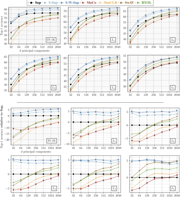
the first 32, 64, 128, 256, 512 and 1024 principal components from the training data available on each concept domain, and transform both the training and test sets to these principal components. Then, we follow our LogReg protocol and learn linear classifiers on each of these transformed data. Results. We show our results in Fig.8(and also provide raw scores in Tab.5), and observe the following.

(a) Interestingly, supervised classifiers do a pretty good job in learning compact spaces of visual features, which are not only useful for the seen concepts but also for the unseen concepts to some extend. For instance, on IN-1K supervised classifiers need only the first 32 principal compo-nents to achieve+63% accuracy by LogRegs. Moreover, on L1/2/3/4, supervised classifiers can capture more discrimi-native patterns for the unseen concepts into the first 32 and 64 principal components compared to the self-supervised models.

(b) Surprisingly, the performance of Sup starts to saturate after the first 128 principal components on all concept do-mains, i.e., the more principal components bring diminishing improvements after the first 128 of them. Moreover, the first 1024 and 2048 principal components contribute equally to the transfer learning performance of Sup on all concept do-mains. This indicates that half of the principal components does not provide any variance for the features learned by Sup that is useful to discriminate the concepts.

(c) Contrarily, self-supervised models consistently im-prove until all the principal components are used (in log-scale), showing that the overall variance of the features are captured by more principal components.

C.3. ...by non-linear classifiers

Although linear classification has been the standard way of evaluating the transfer learning performance for pretrained models, they are limited in terms of their expressivity: they expect features extracted for the unseen concepts to be lin-early separable in the high-dimensional embedding space that was learned on the seen concepts. Although this as-sumption holds up to some point, i.e., the models achieve +49% top-1 accuracy on L5(see Tab.2), in Fig. 3.c of the main paper we can clearly see sharp relative performance drops for all models immediately starting fromL1. Could those drops be the result of the strong linear separability assumption?

Inspired by the success of applying a non-linear projec-tion head when learning self-supervised models [2,8–10,20], we further investigate what happens if we relax the linear separability requirement in our previous analysis, and learn multi-layer perceptrons (MLPs) instead.

Concretely, in this setting, we learn MLPs with 2 hid-den layers each having 2048 hidhid-den units and a ReLU non-linearity in between them. Given features x_{∈ R}2048, each MLP outputs 1000-dimensional class logits s =

W3ρ(W2ρ(W1x+ b1) + b2), where W1 and W2 _∈ R2048×2048, b1and b2∈ R2048are the hidden layer param-eters, W3 _{∈ R}1000×2048are the parameters of the output layer, andρ(·) is the element-wise ReLU activation.

Recall that in LogRegs, we apply`2-normalization to the features x to prevent any bias towards the magnitudes of the features (we discuss this in Sec. 3.4 of the main paper). However, we argue that MLPs can adapt to the differences in the magnitudes of the features (if they need to), therefore we do not employ`2-normalization in MLPs.

A direct performance comparison between a LogReg and its MLP counterpart is unfair: the MLP contains millions of extra learnable parameters. Therefore, we also implement MLPNoAct., which is the MLP with no activation function (i.e.,ρ is the identity function), and compare a MLP with its MLPNoAct.counterpart.

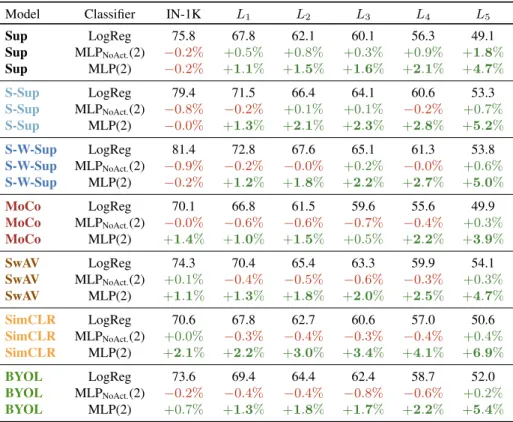
Results. In Tab.3, we show the relative performances of MLPs and MLPNoAct.s over their LogReg counterpart. We observe the followings.

(a) As expected, MLPs do not improve the classifica-tion performance of the supervised models on IN-1K; Be-cause these models are already trained on IN-1K with an objective that linearly separates classes in their feature spaces. However, MLPs do improve the performance of the self-supervised models on IN-1K, i.e.,1.4%, 1.1%, 2.1% and0.7% relative improvements over LogRegs forMoCo, SwAV,SimCLRandBYOL, respectively.

(b) Overall, the MLPs provide consistent gains for all models on our concept generalization levelsL1/2/3/4/5. Sur-prisingly, MLPs are most useful for semantically less similar target domains, e.g., we see significant improvements onL4 andL5 for all models. This supports our motivation that in the feature spaces, which are learnt on the seen classes, the semantically dissimilar unseen classes are not strictly linearly separable.

(c) The gains of MLPs are largely due to its non-linearity, i.e., ReLU activations inside. We see that MLPNoAct.s are on par or worse than their LogReg counterparts, except for Sup, for which MLPNoAct.s also improve significantly.

D. Topology of feature spaces

In Sec. 4.3 of the main paper, we study the topology of the learnt feature spaces for each concept domain (IN-1K and our levelsL1/2/3/4/5). We extend this analysis in the following two sub-sections (Sec.D.1, Sec.D.2).

D.1. Clustering evaluation metrics

To understand the clustering quality of the features on each concept domain, we report cluster purity scores ob-tained by each model in Sec. 4.3.1 of the main paper. As we explain in Sec. 3.4 of the main paper, clustering evaluation protocol consists of three steps. First, we learn cluster cen-troids in 2048-dimensional learnt feature spaces using the

Sup S-Sup S-W-Sup MoCo SimCLR SwAV BYOL 32 64 128 256 512 1024 2048 d principal components 40 45 50 55 60 65 70 75 80 T op-1 accuracy IN-1K 32 64 128 256 512 1024 2048 40 45 50 55 60 65 70 L1 32 64 128 256 512 1024 2048 40 45 50 55 60 65 L2 32 64 128 256 512 1024 2048 35 40 45 50 55 60 65 L3 32 64 128 256 512 1024 2048 35 40 45 50 55 60 L4 32 64 128 256 512 1024 2048 30 35 40 45 50 55 L5 32 64 128 256 512 1024 2048 d principal components −20 −15 −10 −5 0 5 T op-1 accuracy relativ e to Sup. IN-1K 32 64 128 256 512 1024 2048 −10 −5 0 5 L1 32 64 128 256 512 1024 2048 −5 0 5 L2 32 64 128 256 512 1024 2048 −5 0 5 L3 32 64 128 256 512 1024 2048 −5 0 5 L4 32 64 128 256 512 1024 2048 0 5 L5

Figure 8: (PCA + LogReg, full data.) Top-1 accuracy for each method (pretrained on IN-1K) obtained by logistic regression classifiers (LogReg). First, we apply PCA to reduce the dimensionality of the pre-extracted features for the concepts in IN-1K and our generalization levelsL1/2/3/4/5. We compute the principal components using all training samples available for the concepts, i.e.,N = All, then apply them to both training and test samples. Second, we train each LogReg on the compressed features. “2048”, the performance when all the principal components are used, is also shown for reference. Top two rows; from left to right and top to bottom: results obtained on IN-1K and our concept generalization levelsL1/2/3/4/5. Bottom two rows: the same data as the top two rows, but now all accuracies are relative to Sup.

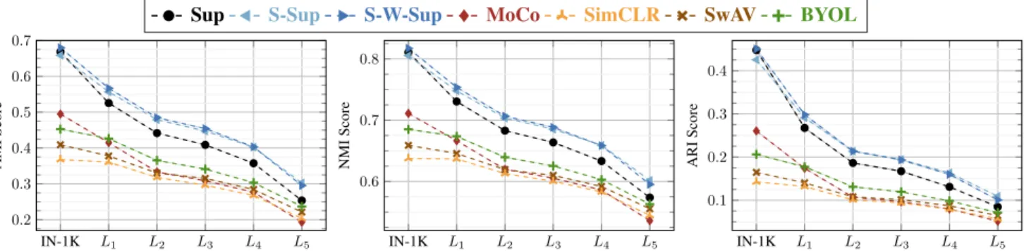
Sup S-Sup S-W-Sup MoCo SimCLR SwAV BYOL IN-1K L1 L2 L3 L4 L5 0.2 0.3 0.4 0.5 0.6 0.7 AMI Score IN-1K L1 L2 L3 L4 L5 0.6 0.7 0.8 NMI Score IN-1K L1 L2 L3 L4 L5 0.1 0.2 0.3 0.4 ARI Score

Figure 9: From left to right adjusted mutual information (AMI), normalized mutual information (NMI) and adjusted rand-index (ARI) scores between the cluster assignments predicted byk-Means and the concept labels, computed on the test set of each level. Adjusted denotes that corresponding scores are adjusted for chance.

training set of each concept domain, Second, we assign the corresponding test samples to the cluster centroids, Third we compute the purity scores of the test samples based on their concept labels and cluster assignments.

To compute purity scores, we first compute the confusion matrix_{M between the labels and cluster assignments of} the test samples such that_Mij denotes the number of test samples belonging to concepti and assigned to cluster j. Then the purity score is computed as

purity= 1 1000 1000 X i=1 max({Mij| j = {1, . . . , 1000}}). (3) In this section, we provide additional results obtained by other popular clustering evaluation metrics, i.e., ad-justed [60] and normalized mutual information, and adjusted rand-index [46] scores in Tab.6. Adjusted denote that these metrics are adjusted for chance, so that random permutations result in scores close to 0. We compute these metrics using the implementations available in scikit-learn [45].

We observe that the overall behavior of the models is consistent across all of the metrics considered.

D.2. Alignment and uniformity scores

To understand the spread of the features for the unseen concepts, in Sec. 4.3.2 of the main paper, we measure their alignment and uniformity scores, both based on the pairwise relationships of the features [64]. We only provided the alignment over uniformity scores computed on our levels L1/2/3/4/5 that are relative to IN-1K. In Fig.10, we also report alignment and uniformity scores obtained by each model on each concept domain.

E. ImageNet-CoG constructed with word2vec

One of the requirements for studying concept general-ization in a controlled manner is a knowledge base that provides the semantic relatedness of any two concepts. As

ImageNet [13] is built on the concept ontology of Word-Net [41], in Sec. 3.3 of the main paper we make use of the graph structure of WordNet, and we propose a bench-mark where semantic relationships are computed by the Lin measure [35].

As we mention in Sec. 3.1 of the main paper, the WordNet ontology is hand-crafted requiring expert knowledge. There-fore similarity measures that exploit this ontology (such as Lin) are arguably reliable in capturing the semantic simi-larity of concepts. However, it could also be desirable to learn semantic similarities automatically, for instance, using knowledge bases available online such as Wikipedia. In this section, we investigate if such knowledge bases could be used in building our ImageNet-CoG.

With this motivation, we turn our attention to semantic similarity measures that can be learned over textual data describing the ImageNet concepts. Note that each ImageNet concept is provided with a name1_{and a short description}2_. So, the idea is to use these information to determine the semantic relatedness of any two concepts.

To do that, we consult language models to map textual data for any ImageNet concept into an embedding vector, such that semantic similarities of the concepts are absorbed in the embedding space. To achieve this, we use the skip-gram language model [40], which has been extensively used in many natural language processing tasks, to extract “word2vec” representations of all ImageNet concepts.

How-ever, we note that the name of many ImageNet concepts are named entitiescomposed of multiple words, yet the vanilla skip-gram model tokenizes a textual sequence into words. To address this, we use the extension proposed by [71] that learn a skip-gram model by taking into account such named entities. More specifically, we use the skip-gram model trained on Wikipedia3_{by the Wikipedia2Vec software [70].} To compute the word2vec embeddings of the ImageNet

1_{http://www.image-net.org/archive/words.txt} 2_{http://www.image-net.org/archive/gloss.txt} 3_{April 2018 version of the English Wikipedia dump.}