Case studies in quantum adiabatic optimization

Case Studies in Quantum Adiabatic Optimization

by

David Gosset

Submitted to the Department of Physics

in partial fulfillment of the requirements for the degree of

Doctor of Philosophy

at the

MASSACHUSETTS INSTITUTE OF TECHNOLOGY

ARCHIVES

MASSACHU _{iNs rTJUTE}

OF TECHNOyLYr

L B31201

1

L 1

1DAR

I

ES

June 2011

@

Massachusetts Institute of Technology 2011. All rights reserved.

'/ X

A u th or ...

artent

of Physics

May 20, 2011

Certified by...

Edward Farhi

Cecil and Ida Green Professor of Physics

Thesis Supervisor

-9/.

'0/

Accepted by ... /...

Krishna Rajagopal

Professor of Physics

Associate Head for Education, Physics

Case Studies in Quantum Adiabatic Optimization

by

David Gosset

Submitted to the Department of Physics on May 20, 2011, in partial fulfillment of the

requirements for the degree of Doctor of Philosophy

Abstract

Quantum adiabatic optimization is a quantum algorithm for solving classical optimization problems (E. Farhi, J. Goldstone, S. Gutmann, and M. Sipser. Quantum computation by adiabatic evolution, 2000. arXiv:quant-ph/0001106). The solution to an optimization prob-lem is encoded in the ground state of a "probprob-lem Hamiltonian" Hp which acts on the Hilbert space of n spin 1/2 particles and is diagonal in the Pauli z basis. To produce this ground state,

one first initializes the quantum system in the ground state of a different Hamiltonian and then adiabatically changes the Hamiltonian into Hp. Farhi et al suggest the interpolating Hamiltonian

i

where the parameter s is slowly changed as a function of time between 0 and 1. The running time of this algorithm is related to the minimum spectral gap of H(s) for s E (0, 11.

We study such transverse field spin Hamiltonians using both analytic and numerical techniques. Our approach is example-based, that is, we study some specific choices for the problem Hamiltonian Hp which illustrate the breadth of phenomena which can occur. We present

I A random ensemble of 3SAT instances which this algorithm does not solve efficiently. For these instances H(s) has a small eigenvalue gap at a value s* which approaches 1

as n - oc.

II Theorems concerning the interpolating Hamiltonian when Hp is "scrambled" by conju-gating with a random permutation matrix.

III Results pertaining to phase transitions that occur as a function of the transverse field.

IV A new quantum monte carlo method which can be used to compute ground state prop-erties of such quantum systems.

We discuss the implications of our results for the performance of quantum adiabatic opti-mization algorithms.

Thesis Supervisor: Edward Farhi

Acknowledgments

Let me begin by thanking Eddie who taught me most of what I learned at MIT: a good amount of quantum computation but more importantly how to think about physics.

I especially thank Eddie for all the fun and intellectually challenging meetings and

for generally being an outstanding advisor and friend. It has been a great privilege to work closely with Eddie, Jeffrey Goldstone, Sam Gutmann and Peter Shor.

I also thank Eddie and Sam for encouraging my obsession with ice hockey. I thank Stephen Jordan, Avinatan Hassidim, Daniel Nagaj and Andy Lutomirski

for being exemplary collaborators and friends.

Harvey Meyer's expertise in Monte Carlo simulation was an invaluable asset during our projects together and I thank him for sharing his knowledge and experience.

I thank Scott Aaronson and Isaac Chuang and Peter Shor for their classes in

quantum information which I enjoyed and benefitted from.

I thank Laura Foini, Florent Krzakala, Guilhem Semerjian and Francesco Zamponi

for their expert opinions and for answering many questions I have had about the cavity method and other topics. I have learned a great deal from them and greatly appreciated their hospitality during my visit to Paris.

I thank Steve Flammia, Itay Hen, Jon Kelner, Chris Laumann, Peter Love,

Hart-mut Neven, and Peter Young for many interesting discussions.

I thank NSERC, the W.M Keck foundation, the MIT-France program, and Curt

and Kathy Marble for financial support.

I thank my friends Nick Herman, Mike Matejek and Dave Shirokoff.

I am grateful to my family. My parents for encouraging me to study physics and

for steering me to do my best. My siblings John, Laura and Paul for always being fun, interesting, and smart.

Finally I thank Anne with whom I have shared most of my life and who has been a source of unflagging support and inspiration. Thanks for all of the time we have spent together and for making the best of the time we have been living apart.

Contents

1 Introduction ₁₃

1.1 _{Performance of Quantum Adiabatic Algorithms . . . . 16}

1.1.1 _{Grover and Scrambled Problem Hamiltonians . . . . 16}

1.1.2 Cost Functions which depend only on the Hamming W eight . . . . 20

1.1.3 _{Clause Based Decision Problems . . . . 22}

1.1.4 Quantum Adiabatic Algorithms and Phase Transitions . . . . 30

1.2 Tools for Stoquastic Hamiltonians . . . . 31

1.2.1 _{N o N odes . . . .} 32

1.2.2 _{A Variational Lower Bound For the Ground State Energy . . . 33}

1.2.3 _{The Continuous Imaginary Time Path Integral and a} Probabil-ity Distribution over Paths . . . . 34

1.2.4 Quantum Monte Carlo and The Quantum Cavity M ethod . . . . 36

1.3 _{The Next Four Chapters . . . . 37}

1.4 _{O utlook . . . . 38}

2 A Quantum Monte Carlo Method at Fixed Energy 2.1 _{Introduction . . . .} 2.2 The Ham iltonian . . . . 2.3 _{Description of the method . . . .} 2.4 Sampling Paths for Transverse Field Spin Hamiltonians . . 2.5 _{Two Observations . . . .} 2.5.1 A New Estimator for the Ground State Energy for Path 41 . . . . . 41 . . . . . 44 . . . . . 45 . . . . . 47 . . . . . 52 Integral Quantum Monte Carlo . . . .

2.5.2 _{A Variational Ansatz for the Ground State . . . .}

2.6 _{C onclusions . . . .} 3 Perturbative Crosses

3.1 Problematic Instances . . . .

3.2 _{Fixing the Problem by Path Change . . . .}

3.3 Quantum Monte Carlo Simulations . . . .

3.3.1 Equilibration of the Quantum Monte Carlo and

of Level Crossings . . . . 3.3.2 Randomizing the Beginning Hamiltonian . . . .

3.3.3 Data for an Instance of 3SAT with 150 bits . . . . 66

3.4 Conclusions . . . . 68

3.5 Num erical Results . . . . 68

4 Scrambled Hamiltonians and First Order Phase Transitions 85 4.1 Scrambled Hamiltonians . . . . 85

4.2 R esults . . . . 86

4.3 Variational Ansatzes for the Ground State of H,(s) . . . . 87

4.4 Discussion and Conclusions . . . . 89

4.4.1 Connection to Previous work on Random Energy Models . . . 91

4.5 Proofs . .... . . . . 91

5 Phase Transitions in 3XORSAT and Max-Cut 101 5.1 Introduction . . . . 101 5.2 3-Regular 3XORSAT . . . . 103 5.2.1 Duality M apping . . . . 104 5.3 3 Regular M ax-Cut . . . . 105 5.3.1 Numerical Results . . . . 106 5.4 D iscussion . . . . 110

A Estimators in the Continuous Imaginary Time Ensemble of Paths 113 B Algorithm for Sampling from the Single Spin Path Integral 117 C Analysis and Derivation of Estimators at Fixed Energy 121 D Convergence of The Markov Chain 125 E The Quantum Cavity Method 129 E.1 The Quantum Cavity Method For a Two local Transverse Field Spin Hamiltonian on a Tree . . . . 129

E.2 1RSB Quantum Cavity Equations with Parisi Parameter m = 0 . . . 132

List of Figures

1-1 (From [13]) Lowest 25 levels for the unscrambled Hamiltonian H at n = 18 . . . . 17

1-2 (From [13]) Lowest 25 energy levels for an instance of the scrambled Hamming weight problem H,(s) with a random permutation at n = 18. The inset shows a magnified view of levels 2 through 19 near s = 0.6. 18 1-3 The two lowest energy levels near s = 1 before (left) and after (right)

adding the final penalty clause. A "perturbative cross" is created by adding this single clause which breaks the degeneracy between two local m inim a. . . . . 27

1-4 The energy per spin for (satisfiable) 2XORSAT on a ring. . . . . 31

2-1 Eg(A) for the Hamiltonians we consider. As A -± ±oo we have Eg -+ -oo. 45 2-2 Monte Carlo update where the order of 2 flips in the path is interchanged. 48

2-3 Monte Carlo update where 2 adjacent flips in the path which occur in

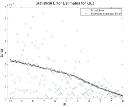
the same bit are replaced by flips in a different bit. . . . . 49 2-4 A(E) computed using Monte Carlo data and exact diagonalization for a

16 spin Hamiltonian. Statistical error bars are included for the Monte

Carlo results, but they are barely visible. We have also plotted the errors separately in Figure 2-6 . . . . 50 2-5 -A(E)(Og(A(E))|Vl~g(A(E))) computed using Monte Carlo data and

exact diagonalization for a 16 spin Hamiltonian. Statistical error bars are included for the Monte Carlo results, but they are barely visible. Errors are also plotted separately in Figure 2-7. . . . . 50 2-6 A(E) from Figure 2-4. The black crosses show the estimated statistical

error. The blue circles show the magnitude of the difference between the Monte Carlo estimates and the result of exact numerical diagonal-ization . . . . 5 1

2-7 -A(E)(/g(A(E))|Vl)g(A(E))) from Figure 2-5. The black crosses show

the estimated statistical error. The blue circles show the magnitude of the difference between the Monte Carlo estimates and the result of exact numerical diagonalization. . . . . 51

3-1 A true energy level crossing can arise from two disconnected sectors. . 58

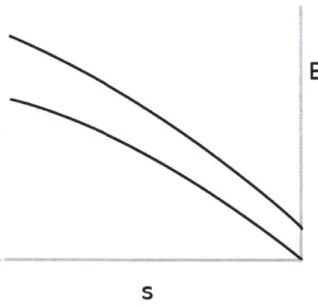
3-2 s = 1. Here the second derivative of the upper curve B is greater than

3-3 The discontinuity in the circle data that occurs near s = 0.4 is a Monte Carlo effect that we understand. As can be seen from the exact numerical diagonalization there is no true discontinuity in either the ground state energy or the first excited state energy. For s greater than 0.4 the Monte Carlo simulation is in a metastable equilibrium that corresponds to the first excited state. The true ground state energy at each s is always the lower of the circle and the cross at that value of s. . . . . 69

3-4 Together with Figure 3-3, we see that the discontinuity in the circles appears in data for both the energy and the Hamming weight. This is not indicative of a phase transition in the physical system (as evidenced

by the smooth curves computed by exact numerical diagonalization),

but is purely a result of the way in which we use the Monte Carlo m ethod . . . . 70 3-5 After adding the penalty clause we see that the energy levels have

an avoided crossing at s e 0.423. The inset shows exact numerical diagonalization near the avoided crossing where we can resolve a tiny gap. The ground state energy is well approximated by the lower of the circle and cross at each value of s. . . . . 71 3-6 In this Figure there is a phase transition which occurs near s d 0.423.

We see from the exact numerical diagonalization that the Hamming weights of the first excited state and ground state undergo abrupt transitions at the point where there is a tiny avoided crossing in Figure

3-5. There is also a jump in the Monte Carlo data plotted with circles

that occurs before the avoided crossing: this is a Monte Carlo effect as discussed earlier and has no physical significance. If we look at the Monte Carlo data in Figure 3-5 we conclude that below s r 0.423

the crosses represent the ground state and after this point the circles represent the ground state. From the current Figure, along with Figure

3-5, we conclude that the Hamming weight of the ground state jumps

abruptly at s* a 0.423. . . . . 72 3-7 (2) (2) for 1 million different choices of coefficients ci shows a

substan-tial tail for which 27 -

s2

(> 0. These sets of coefficients correspond

to beginning Hamiltonians HB for which we expect the small gap in Figure 3-5 to be removed. . . . . 73 3-8 A random beginning Hamiltonian removes the crossing seen in Figure

3-5. The problem Hamiltonian is the same as that in Figure 3-5. The

circles are always below (or equal to) the crosses for all values of s. This means that the circles track the ground state for all s and we see no sign of a small gap in the Monte Carlo data. This is consistent with the displayed exact numerical diagonalization. . . . . 74

3-9 From Figure 3-8 we see that the ground state of the Hamiltonian

corre-sponds to the circles for all values of s and the Hamming weight of the circles here goes smoothly to the Hamming weight of the unique satis-fying assignment. (The jump in the Monte Carlo data corresponding to the crosses is due to the Monte Carlo effect discussed earlier.) . . . 75

3-10 The crosses, which represent the Monte Carlo data seeded with 111...1,

are below (or equal to) the circle data for all values of s. (This is seen more clearly in the inset which shows the positive difference between the circle and cross values). We conclude that the crosses track the ground state energy which is smoothly varying. The jump in the circle data is a Monte Carlo effect and for s above 0.2 the circles track the first excited state. _{. . . .} 76 3-11 Comparing with Figure 3-10 we see that the Hamming weight for the

first excited state and the ground state are continous functions of s . We only obtain data for the first excited state for values of s larger than s e 0.2 . . . . 77 3-12 Adding the penalty clause makes the cross data go above the circle

data at s - 0.49. This is shown in more detail in Figure 3-13 where we plot the energy difference between the first two levels as a function of s. We interpret this to mean that the Hamiltonian H(s) has a tiny gap at s* a 0.49. . . . . 78 3-13 The energy difference, circles minus crosses, from Figure 3-12 near the

value of s where the difference is 0. Note that second order perturbation theory does quite well in predicting where the difference goes through

zero. ... ... 79

3-14 Looking at Figure 3-12 we see that the ground state is represented by the crosses to the left of s ~ 0.49 and is represented by the circles after this value of s. Tracking the Hamming weight of the ground state, we conclude that it changes abruptly at s e 0.49. . . . . 80

3-15

e

- )( for 100000 choices of coefficients ci for our 150 spin instance.

Note that a good fraction have e -

e

> 0. . . . . . . . . 81

3-16 A random choice of coefficients such that

e

-

e2

> _ gives rise to

an H(s) where there is no longer an avoided crossing. The circles here correspond to the ground state for all s since the cross data is always above (or equal to) the circle data for all s. This can be seen in the inset where we have plotted the energy difference, crosses minus circles. The crosses have a Monte Carlo discontinuity near s 0.2, after which they correspond to the first excited state. . . . . 82 3-17 Looking at Figure 3-16 we see that the ground state corresponds to the

circles for all values of s so we see here that the Hamming weight of the ground state goes smoothly to its final value as s is increased. We take this as further evidence that this choice of HB would correspond to success for the quantum adiabatic algorithm for this instance. . . . 83

5-1 The black dots show the energy per spin for 3 Regular Max-Cut at

#

= 4 computed in the 1RSB cavity method with Parisi parameter

m = 0 as a function of transverse field A. The inset shows the behaviour

near A = 0 . The blue circles show numerical diagonalization results for the ground state averaged over 50 random instances of Max-Cut on 16 bits which are restricted to the subset which have exactly two degenerate lowest energy states with energy per spin equal to -1.25. The red asterisks show numerical diagonalization results for the ground state averaged over 50 random instances of Max-Cut on 24 bits with exactly two degenerate lowest energy states with energy per spin equal to - 1.25 . . . . 108 5-2 The black dots show the Edwards Anderson order parameter computed

with the 1RSB cavity method with m = 0 at

#

= 4. The blue dots show the order parameter qp in the ground state, averaged over 50 random instances of Max-Cut on 16 bits which are restricted to the subset which have exactly two degenerate lowest energy states with energy per spin equal to -1.25. The red dots show the order parameter qp in the ground state, averaged over 50 random instances of Max-Cut on 24 bits which are restricted to the subset which have exactly two degenerate lowest energy states with energy per spin equal to -1.25. . 109 5-3 The magnetization along the transverse direction computed with the

1RSB cavity method with m = 0 at

#

= 4. The inset shows the region around the phase transition. . . . . 109

E-1 The subtree T M . . . . 131

E-2 The energy density computed with the cavity method at

#=

4 and

two different values of NR. Note that the value at A = 0 differs very

slightly between the two data runs. . . . . 137 E-3 The Edwards Anderson order parameter computed with the cavity

method at

#

= 4 and two different values of NR. . . . . 138 E-4 The x magnetization computed with the cavity method at

#

= 4 and

Chapter 1

Introduction

The subject of this thesis is the quantum adiabatic algorithm[21], which is a quantum algorithm for solving optimization problems.

Are there optimization problems which the quantum adiabatic algorithm can solve faster than the best classical algorithm? Answering this question is the objective of research on quantum adiabatic algorithms. It is a very difficult open question.

In this thesis we study the performance of the quantum adiabatic algorithm, focusing on a set of examples where we are able to make progress. The goal is to understand where to look for optimization problems on which the adiabatic algorithm performs well. Along the way we will develop technical tools which can be used to study transverse field quantum spin systems. We hope that the reader with some knowledge of classical and quantum computation (having perhaps already studied the standard text [521) will find this thesis accessible.

We now describe the quantum adiabatic algorithm [21].

The Quantum Adiabatic Algorithm

The optimization problems to be solved have the following form. Given a cost function

f(z) which assigns a real number to each n-bit string, the goal is to find the bit string

zo which minimizes f. Assume for simplicity that f(z) > f(zo) for z f zo.

A first step in describing the quantum adiabatic algorithm is to rephrase the

optimization problem to be solved. Consider the Hilbert space of n spin j particles. Write each Pauli z-basis state of the n spin system as a bit string, where 0 is spin up and 1 is spin down. Then define the "Problem Hamiltonian"[21]

H = f (z) z)Kz| (1.1)

which has the property that the ground state of this Hamiltonian is the basis state |zo) corresponding to the bit string we are looking for.

Now let's suppose that we actually have a quantum system of n spin I particles, and that we're able to control the Hamiltonian of the system. A simple version of the quantum adiabatic algorithm works as follows.

We assume that we can prepare a product state of the n spins

I VB) 0) +11) *n

Start by setting the Hamiltonian of the system to be

HB 2 x) (1.2)

-which we call the beginning Hamiltonian[21], and initialize the state of the n spins in the state JOB) which is the ground state of this Hamiltonian. Then slowly change the Hamiltonian of the system over a time T so that, at the end of the evolution, the Hamiltonian has been changed to Hp.

We now review the quantum adiabatic theorem (see for example [45]) which applies to very slowly changing Hamiltonians. Consider a Hamiltonian H(s) which depends on a parameter s

E

[0, 1] and which has a unique ground state at each value of s. The

quantum adiabatic theorem can be applied under some fairly general conditions on the Hamiltonian H(s). Suppose that we initialize a quantum system in the ground state |0(0)) of the Hamiltonian H(0) and then change the Hamiltonian H(s) as a function of time along the path s(t) =. The quantum system evolves according to the Schr6dinger equation

dt

(setting h = 1). The quantum adiabatic theorem says that, for any s E [0, 1], by

taking T large enough the state |@(sT)) can be made arbitrarily close to the instan-taneous ground state of H(s).

In the quantum adiabatic algorithm we take the interpolating Hamiltonian

H(s) = (1 - s) HB + sHp (1.4)

where s(t) =. So if we choose T large then at the end of the time evolution the quantum system will be very close to the ground state of Hp. After the adiabatic evolution, the quantum system is measured in the Pauli z basis. Since the quantum system is very close to the state

Izo)

this measurement will likely result in the output bit string zo which solves the optimization problem of interest.

From the adiabatic theorem we know that the quantum adiabatic algorithm pre-pares the state |zo) in the limit T -- o. How big does T have to be to get a

probability of finding the state |zo) at the final measurement which is larger than some fixed threshold probability p? (A constant success probability is good enough because it can be amplified by running the algorithm independently a fixed number of times). The finite running time behaviour of quantum adiabatic evolution is governed

by the adiabatic approximation which tells us how large to make T in order to get

given in reference [32].

A simpler question is that of computational efficiency. An efficient algorithm has

a running time which grows as a polynomial function of the input size (in this case

n), whereas an inefficient algorithm has a running time which is superpolynomial

in n. Computational efficiency is a crude but useful measure of whether or not an algorithm is scalable in practice. For which problems is the quantum adiabatic algorithm efficient? It turns out that to answer this question the relevant property of the interpolating Hamiltonian 1.4 is the minimum spectral gap

gmin = min [ (Ei(s) - Eo(s))

SE0,1]

where EI(s) is the first excited state energy and Eo(s) is the ground state energy. Let us assume that the norm of the Hamiltonian H(s) is upper bounded for all s

by a polynomial function of n. Then the adiabatic approximation tells us that the

quantum adiabatic algorithm is efficient when gmin is asymptotically larger than an inverse polynomial in n [211. On the other hand if gm is exponentially small as a function of n then the adiabatic algorithm will be inefficient.

We now comment briefly on our motivation for studying quantum adiabatic op-timization. As we have already mentioned, the primary goal is to look for problems on which the quantum adiabatic algorithm outperforms classical algorithms. Other quantum algorithms such as Shor's algorithm [59] for factoring integers and Grover's algorithm [26] for unstructured database search are remarkable because the running time of these algorithms is asymptotically faster than the running time of the best classical algorithm to date (in the case of factoring integers) or the best possible clas-sical algorithm (in the case of unstructured database search) for the same task. These quantum algorithms were developed in the "circuit model" of quantum computation-a stcomputation-andcomputation-ard theoreticcomputation-al frcomputation-amework for qucomputation-antum computation-algorithms. Qucomputation-antum computation-adicomputation-abcomputation-atic op-timization is a different approach (although quantum adiabatic opop-timization with a local Hamiltonian can be simulated efficiently by a traditional quantum computer) and we do not yet know of any quantum speedups using this method.

A second reason to study quantum adiabatic optimization is to better understand

the computational limitations which are imposed by the specific form of the interpo-lating Hamiltonians used. Transverse field spin Hamiltonians have a special property called stoquasticity [10] which means that all off diagonal matrix elements are nonpos-itive. As we will see in section 1.2, this special property can be exploited by various classical algorithms which simulate the quantum system of interest. Whether or not quantum adiabatic evolution with a stoquastic local Hamiltonian can be efficiently simulated on a classical computer is an open question (no such efficient simulation technique exists to date). Studying quantum adiabatic optimization by example may give some insight into the similarities and differences between quantum adiabatic op-timization and classical opop-timization methods. We return to this point in section 1.4.

The rest of this Chapter is organized as follows. In section 1.1 we review some problems where it has been possible to determine the running time of the adiabatic

algorithm. In our discussion we will preview some of the examples which are treated in subsequent Chapters. In section 1.2 we introduce the numerical and analytic techniques that we will use in this thesis. Finally, in section 1.3 we give an outline of the rest of the thesis. In section 1.4 we conclude with an overview of complexity theoretic considerations which are relevant to the quantum adiabatic algorithm.

1.1

Performance of Quantum Adiabatic Algorithms

In this section we review progress towards understanding the running time of quantum adiabatic algorithms.

The first examples we review in section 1.1.1 all have the property that the function to be minimized has very little structure. In these cases it has been proven that the

quantum adiabatic algorithm cannot succeed in subexponential time [17, 16].

We then discuss the case[15, 21, 19] where the function to be minimized only depends on the Hamming weight of its argument (an n bit string). In section 1.1.2 we review the strategy introduced in references [19, 21, 15] for analyzing the quantum adiabatic algorithm applied to such problems.

In section 1.1.3 we review results that pertain to quantum adiabatic algorithms for clause based decision problems such as 3SAT, Exact Cover, and XORSAT.

We conclude in section 1.1.4 with a discussion of the relationship between phase transitions and quantum adiabatic algorithms.

1.1.1

Grover and Scrambled Problem Hamiltonians

Grover's algorithm [27] is a quantum algorithm (originally defined in the circuit model of quantum computation) which solves the following problem. The goal is to find a special bit string zo out of the 2" possible n-bit strings. In order to determine the bit string zo we are allowed to make queries to an "oracle" which takes as input a given bit string y and outputs "yes" if y = zo and "no" otherwise. This oracle is given to

the user as a "black box" unitary transformation.

A different version of Grover's problem where the oracle is given as a Hamiltonian

was defined in [17]. Here we are given the problem Hamiltonian

Hp = 1 -

Izo)(zol

(1.5)

as a "black box" which we are allowed to apply to our system, and the goal is to find

zo. The quantum adiabatic algorithm with interpolating Hamiltonian H (s) n 1 - o f

H~s = 1 -s)2 + S (1 - Izo)(zol)

was studied in [21] where it was shown that for this problem the minimum gap is asymptotically ~ 2 . 2- and the running time of the adiabatic algorithm is

W 2.5-2 1.5-0.5 0.1 0.2 0.3 0.4 0.5 0.6 0.7 0.8 0.9 S

Figure 1-1: (From [13]) Lowest 25 levels for the unscrambled Hamiltonian HE at

n = 18.

bounds for solving Grover's problem within a more general "continuous time" model of quantum computation).

An extension of these results was given in [16] where it was shown that quantum adiabatic optimization cannot achieve success in subexponential time when the be-ginning Hamiltonian HB is a rank 1 projectdr (as opposed to the Grover case where the problem Hamiltonian is rank 1).

Reference [16] also discussed quantum adiabatic algorithms for a class of problem Hamiltonians Hp which are "scrambled". Given a function h(z) defined over the set of n bit strings and a permutation 7r _{which permutes the set of all 2n n-bit strings,}

define

h,(z) = h(7r-'(z)).

Each permutation 7r corresponds to a particular scrambled function h,, so there are 2"! possible scrambled functions.

In [16] it was proven that the quantum adiabatic algorithm cannot efficiently find the bit string which minimizes h, for a randomly chosen 7r (with high probability over the choice of 7r) [16]. The theorem proven in [16] applies to a more general class of algorithms. It is (in a slightly adapted form)

W _4.05 2.5-2-4 1.5-3.9 0.6 0.605 0.61 0.615 0.1 0.2 0.3 0.4 0.5 0.6 0.7 0.8 0.9 S

Figure 1-2: (From [13]) Lowest 25 energy levels for an instance of the scrambled

Hamming weight problem H,(s) with a random permutation at n = 18. The inset

Scrambled Theorem (modified from [16]). Let h(z) be a cost function, with

h(O) = 0 and h(1), h(2), ..., h(N - 1) all positive. Let i be a permutation on N ele-ments, and HD(t) be an arbitrary w-independent Hamiltonian. Consider the Hamil-tonian

H(t) = HD(t) + c(t) ( 1 _{h(-1(z))|z)(z)}

where |c(t)| < 1 for all t. Let |@,(T)) be the state obtained by Schrodinger evo-lution governed by H,(t) for time T, with a 7-independent starting state. The bit string which minimizes the scrambled cost function is 7(0) and algorithmic success corresponds with measuring the basis vector

|7(0))

at the end of the Schrodinger time evolution. Suppose that the success probability |(,(T) i(0)) 2 > , for a set of cN!

permutations. Then eNN '256 T > 2V-for N > -.6 - 64h* N -where E Z h*~ (Zh(z)2)2 hN - 1 _) ~

The above simplified version of the theorem bounds the time required to obtain success probability at least _{y 2} -the original theorem from [161 gives a similar bound for any choice of success probability.

The authors of [16] discussed the lessons learned from this result for quantum adiabatic algorithm design. A scrambled function h, leads to a problem Hamiltonian

Hp, = h, (z)Iz)(z z

and the interpolating Hamiltonian

H, (s) = (1 - s) 2 Ori)+ 'SHP, .(16

i=1

In the quantum adiabatic algorithm s s(t) is changed as a function of time. The

Scrambled Theorem can be applied with the identifications c(t) = s(t) and

HD (t) = (I - s (t)20 1.7)

An example considered in [16] is where h(z) computes the Hamming weight (num-ber of ones) of the bit string z. In that case the unscrambled Hamiltonian H,1 (where

I is the identity permutation) is

and the Hamiltonian HE(s) can be written as a sum of n single spin terms with no interactions. It was pointed out in [16] that the Hamiltonian H,(s) for most permu-tations 7 does not have the "bit structure" which is present in the Hamiltonian H,(s). The results of [16] show that the quantum adiabatic algorithm will not succeed on the scrambled Hamming weight problem when the permutation 7 is chosen randomly. This is in contrast to the unscrambled case where the minimum gap of HR(s) is inde-pendent of n and the quantum adiabatic algorithm is efficient. It is argued in [16] that in this example the lack of bit structure is responsible for the failure of the quantum adiabatic algorithm.

It was also noted [16] that in the scrambled Hamming weight case the ground state energy of H,(s) has an interesting generic behaviour for randomly chosen per-mutations 7r. The spectrum of Hp,, does not depend on -r. But the spectrum of the Hamiltonian H,(s) does. In Figure 1-1 we show the spectrum of the decoupled Hamiltonian Hff(s) and in Figure 1-2 the spectrum of the Hamiltonian H,(s) for a random choice of the permutation 7r (these plots are reproduced from [13]). It was pointed out in [16] that as n increases the ground state energy of H,(s) appears to approach two straight lines which meet at s = - (when 7 is chosen randomly). We can see this limiting behaviour already in Figure 1-2.

In Chapter 4 we will return to the subject of scrambled Hamiltonians where we will prove convergence results for the ground state energy and minimum eigenvalue gap for such models. Applying our results to the scrambled Hamming weight problem proves that the ground state energy per spin approaches two straight lines in the limit n -> o0 and that the minimum eigenvalue gap gm for this problem is exponentially small.

1.1.2

Cost Functions which depend only on the

Hamming Weight

Quantum adiabatic algorithms for symmetric cost functions f(z), that is, cost func-tions which depend only on the Hamming weight of their input, have been analyzed in references [15, 21, 19]. The Hamming weight of a bit string z is defined to be the number of ones, and is therefore always an integer between 0 and n. Obviously there is an efficient classical algorithm which finds a bit string zo for which f(z) is minimal: for each

j

E {0,1, ...n} choose a bit string z with Hamming weight

j

and compute

f(zj). The minimum of

f

is then achieved by one of these {z3}. It is not hoped that a quantum adiabatic algorithm achieves a speedup over a classical algorithm for any problem like this. The study of quantum adiabatic algorithms for symmetric cost functions is useful because they can be analyzed easily (as we discuss below), and because the lessons learned may help us understand quantum adiabatic algorithms for more difficult computational problems. We now review the techniques that have been used to study quantum adiabatic algorithms applied to such problems.

Write

H = f (z) z)(z| (1.8)

where f(z) depends only on the Hamming weight of z. If we add to this problem Hamiltonian 1.8 a beginning Hamiltonian

HB=CZ(1 2_7)

(where C is a constant that may depend on n) then the full Hamiltonian

H(s) = (1 - s) HB + sH,

is a function of the total spin operators

2i1

and

Sz =>c0 .

i=1

The operators Sz and Sx both commute with S2 = Sx + Sz2 + S2. It is easy to verify that the Hamiltonian H(s) commutes with S2 since the problem Hamiltonian is a function of Sz and the beginning Hamiltonian is a function of Sx. Because of this symmetry, the ground state of the system remains in the n

+

1 dimensional

symmetric subspace throughout the quantum adiabatic evolution and so the only relevant eigenvalue gap is the gap within this subspace. This gap can be computed using numerical diagonalization up to very large values of n. This strategy has been used to convincingly obtain the asymptotic scaling of the gap with n for a number of different examples[21, 19, 15].

A second approach[15] for analyzing the quantum adiabatic algorithm applied

to a symmetric cost function can be applied when (for large n) the function to be minimized is of the form

W(z)

f(z) = n'V( ) + O(nr-) (1.9)

n

(where W(z) is the hamming weight function and r

E

0, 1, 2, ...) so that in the limit n -± oc the dependence of f on the Hamming weight is captured by the "intensive" function V(u) with a E [0, 1]. This function V(u) is an energy landscape for the problem at s = 1 in the limit n -+ oo. In reference [15] it is shown that one can

extend this quantity to an "effective potential" V(u, s) whose minimum characterizes the ground state at any value of s in the limit n -+ oc (however when s / 1 the quantity a no longer represents the rescaled Hamming weight of a bit string). The behaviour of this potential as a function of s can be used to infer whether or not an exponentially small gap is present for finite size systems[15].

In [19] an algorithmic strategy called "path change" was introduced and applied to symmetric cost functions. For some problem Hamiltonians the linear interpolation

1.4 between the initial Hamiltonian and the problem Hamiltonian may not be a good choice. Path change is the idea of randomly choosing interpolating Hamiltonians

HR(s) which end at the given problem Hamiltonian HR(1) = Hp and running the

quantum adiabatic algorithm for each random choice in the hopes that one of the runs will be successful. In [19] this path change strategy is applied to a symmetrized problem Hamiltonian for which the quantum adiabatic algorithm with the Hamilto-nian 1.4 does not succeed. In that case it is shown [19] that path change can be used to give an efficient quantum adiabatic algorithm for this symmetrized problem. Farhi et al. suggest that path change may be a useful strategy to use with the quantum adiabatic algorithm applied to problems which are not symmetrized. This was the main purpose of introducing path change, since (as we have already discussed) sym-metrized problems are not interesting from a computational point of view. In Chapter

3 we will see an example of path change applied to a non-symmetric problem.

1.1.3

Clause Based Decision Problems

In this section we review results pertaining to the performance of the quantum adi-abatic algorithm on clause based decision problems such as 3SAT and Exact Cover and XORSAT. Unlike in the Grover and Scrambled cases, these problems have clause structure which an algorithm can try to exploit. And unlike symmetrized cost func-tions, there is presumably no simple limiting "energy landscape" for these problems as

n - oo. We begin by giving some examples of these classical computational problems.

Examples of Clause Based Decision Problems

An instance of 3 Satisfiability (3SAT) on n bits is defined as follows. You are given a set of m clauses. A clause is a specific type of constraint on the n bits which is given as a subset {ki, k₂, k3} of the n bits and a 3-bit string s. Each ki C {1, ..., n}

for i E {1, 2, 3} and s E {000, 001, 010, ...111}. A clause is said to be satisfied by an

n-bit string z if Zk, zk2Zk3

#

s, where zi is the ith bit of z. Given the set of m clauses

which specifies an instance of 3SAT, the question is to determine whether or not there exists an n-bit string z which satisfies all of the clauses. 3SAT is a decision problem, meaning the answer is either yes (if the instance is satisfiable) or no (otherwise).

Exact Cover is another example of a clause based decision problem. Like 3SAT, an instance of exact cover is specified by a set of m clauses and the question is to determine if there is an n-bit string z which satisfies all of them. Each clause in this case is represented by a subset ki, k2, k3 of 3 bits. The clause is satisfied by an n-bit

string if

ZkiZk2Zk3 E {100, 010, 001}.

Note that each exact cover clause can be written as a set of 5 3SAT clauses which penalize the bit strings 000, 011, 101, 110, 111 on the given subset of bits.

A third example of a decision problem is called 3XORSAT. Here a clause on bits

ki, k2, k3 is a constraint of the form

where b

E {0,

1} and the symbol

E

indicates the XOR function. The decision prob-lem is to determine whether a set of m given constraints of the form 1.10 can be simultaneously satisfied.

How hard are the computational problems that we have just described? We briefly mention some ideas from complexity theory which help to answer this question. The complexity class NP is the class of decision problems where every "yes" instance has a proof that can be checked efficiently (on a classical computer). In 3SAT a proof consists of the n-bit string z which satisfies all of the clauses. Given this "winning" bit string, we can check that indeed all of the clauses are satisfied by it. For this reason 3SAT is contained in NP. It turns out that any instance of a decision problem in NP can be mapped into a corresponding instance of 3SAT (without expanding the number of input bits by more than a polynomial factor) [38]. This is the statement that 3SAT is NP-hard. A problem such as 3SAT which is both NP hard and in NP is said to be NP complete. Both 3SAT and Exact Cover are NP complete. Most computer scientists believe that there is no subexponential time algorithm which will solve NP complete problems. On the other hand 3XORSAT can be solved in polynomial time on a classical computer. This is the statement that 3XORSAT is in the complexity class P which consists of the set of decision problems that have polynomial time classical algorithms. To see why, note that each clause in 3XORSAT is a linear constraint over the field ]F'. Determining whether or not a set of linear equations have a solution can be solved in polynomial time using linear algebra.

Sometimes we will consider instances of 3SAT or other decision problems which are drawn at random from an ensemble. Properties of such random instances have been studied using methods from statistical mechanics (see [49] for a review). The canonical random ensemble of 3SAT instances is defined as follows. To generate a random instance on n bits, choose each clause uniformly at random but fix the ratio of clauses to bits a =. If a is sufficiently small then the instance will be satisfiable

with high probability. Similarly if a is sufficiently large then a random instance drawn from this ensemble will be unsatisfiable with high probability. It is believed that there is a "phase transition" at a critical value ac which separates a satisfiable phase from an unsatisfiable phase in the thermodynamic limit n -± oc. Random instances with

a close to ac are believed to be computationally difficult for classical algorithms[49]. Similar phase transition phenomena are believed to occur in random ensembles of other clause based decision problems.

Quantum Adiabatic Algorithms for Decision Problems

A clause based decision problem can be turned into an optimization problem that

can be solved by the quantum adiabatic algorithm. The strategy is to search for a bit string z which satisfies all of the clauses, using (for example) the number of violated clauses as a cost function which must be minimized. If the algorithm runs for a time

T and then outputs the satisfying bit string z when the given instance is satisfiable,

then we don't need to worry about what happens when the instance is not satisfiable. We can simply run the algorithm for time T , check if the output z satisfies all the clauses, and conclude that the instance is satisfiable if that is the case. That is why,

for decision problems, we can restrict to the set of satisfiable instances when studying the runtime of the quantum adiabatic algorithm.

Now let's turn to the quantum adiabatic algorithm for 3SAT from [21]. Take each clause (specified by the subset ki, k2, k3 and the 3 bits s= s1S2S3) and form the clause

Hamiltonian

h

- 1 + (-1)816uk ) (1 + (-1)S20k2 ) 1 + (-1 )33

k3

c2 2 2~

Summing the clause Hamiltonians associated with each of the m clauses we get the problem Hamiltonian for the given instance of 3SAT

m

H, = Yhe1.1

c=1

This Hamiltonian is diagonal in the Pauli z basis, and a bit string

Iz)

has energy equal to the number of unsatisfied (violated) clauses. The form of equation 1.11 makes clear the locality of the problem Hamiltonian-it is a sum of terms he where each term hc involves a bounded number of spins (in this case 3). If there is a zero energy state |zo) then the corresponding bit string zo is a satisfying assignment for the instance. If we restrict to instances with a unique satisfying assignment then the eigenvalue gap of the Hamiltonian

H(s)

= (1X)

+

sHp

i=1

at s = 1 is at least 1 and the minimum gap 9min determines the running time of the

quantum adiabatic algorithm.

Of course one can form problem Hamiltonians for other clause based problems

such as Exact Cover or 3XORSAT in a similar manner.

Worst Case Performance for 3SAT

It is known that there are families of 3SAT instances for which the quantum adiabatic

algorithm has running time which is exponential in the system size[61]. We now review the example from [61]. Start with the 3SAT clause which penalizes the bit string 100. This clause is associated with the 3 qubit Hamiltonian

1-0 1+z 1+ 0,

Z IC) 2 _{2 2}

Form a symmetrized instance of 3SAT by including this clause for each of the n3 triplets of qubits

n

i,j,k=1

We have used the prime superscript in the above to indicate that this is an interme-diate step in the construction of the problem Hamiltonian-we will modify H' to

con-struct the final problem Hamiltonian Hp. Since Hp is symmetric under permutations,

it can be written as a function of the Hamming weight operator W =2 (

)

We get

Hp' = (n-W)W2

= n 3 W)( 2

n n

so the rescaled cost function g(u) = (1 - U) U2 (from equation 1.9). This cost function has two satisfying assignments, which correspond to the bit strings 000...0 and 111... 1. It is possible to use the effective potential analysis of

1151

to show that the quantum adiabatic algorithm with Hamiltonian

H(s) = (1 - s) 2 + SHP

will end up in the solution 000...0 corresponding to the minimum at u = 0 as s -* 1. To construct the problem Hamiltonian Hp, add one additional clause to the Hamilto-nian H' which removes the degeneracy and makes 111...1 the global minimum. The quantum adiabatic algorithm requires exponential time to find the winning bit string

111...1 in this example [61].

This example demonstrates that quantum adiabatic optimization does not succeed in the worst case for 3SAT (with the beginning Hamiltonian 1.2 and the problem Hamiltonian which counts the number of violated clauses). On the other hand the performance of the quantum adiabatic algorithm for typical instances of 3SAT (or other combinatorial optimization problems) drawn from a random ensemble has been more difficult to assess.

Performance on Random Instances of 3SAT and Exact Cover

In this section we will discuss results about the performance of the quantum adiabatic algorithm on random instances of clause based optimization problems. Since different studies have occasionally used different random ensembles of instances for the same problem, we will try to be be clear about which random ensemble was used. The reader should be aware that not all the random instances which are discussed here are believed to be hard to solve classically.

The first numerical studies of quantum adiabatic algorithms for random instances of 3SAT [31] and Exact Cover [20] seemed to suggest that the quantum adiabatic algorithm might efficiently solve typical instances of these problems.

The authors of [20] generated random instances of Exact Cover with a unique satisfying assignment and simulated (on a classical computer) the time evolution of the quantum adiabatic algorithm applied to such instances. The random ensemble of instances which they studied was constructed by adding one clause at a time until the number of solutions became < 1. If the final number of solutions after adding the last clause was zero then they started over, and if it was 1 then the instance was

kept. With this technique they were able to study the performance of the adiabatic algorithm up to n = 20. For each n between 10 and 20 they generated 75 random instances and simulated the adiabatic algorithm for each instance. They computed the median time to reach a constant (chosen to be 1/8) success probability and found that this median time was fitted well to a quadratic function of n.

Another numerical study was undertaken by Hogg in

[31].

Hogg studied the

performance of the quantum adiabatic algorithm on random instances of 3SAT near the satisfiability phase transition. These instances are believed to be very difficult for classical algorithms. Hogg found a polynomial scaling of the running time with n for instances with n as large as 24. Hogg noted that, although the minimum gap determines the asymptotic scaling of the quantum adiabatic algorithm, for n < 20 he found using numerical diagonalization that the median of the minimum gap for the instances he considered did not vary too much with n. This led him to add the caveat "Hence, unlike for large n, the cost is not dominated by the minimum gap size and so the values of Fig. 1 may not reflect asymptotic scaling."[31] (referring to his Figure 1 which appeared to show polynomial scaling for the quantum adiabatic algorithm on the random instances he considered).

The reason that Farhi et al and Hogg were limited to studying relatively small systems is that they both used exact numerical techniques which require an expo-nential amount of computer memory. The dimension of the Hilbert space for an n spin quantum system is 2' and computation involving a vector this large becomes difficult as n increases beyond 20 or so. A technique which has been developed to avoid this problem is called Quantum Monte Carlo. For now we will just mention that this method typically has significantly smaller space requirements, and often can be used at much higher bit number than techniques based on matrix or vector manip-ulation. Young et al. [63] were the first to apply Quantum Monte Carlo to the study of the quantum adiabatic algorithm. They studied an ensemble of random instances of Exact Cover with a unique satisfying assignment which are near the satisfiability transition for this problem (the ensemble studied by Young et al differed from the ensemble studied in [20]). They computed the median minimum gap over a set of random instances at each value of n studied, for n as large as 256. They found that this median minimum gap decreased only polynomially with n which supported the notion that the quantum adiabatic algorithm could efficiently solve typical instances drawn from this ensemble.

Despite this seemingly balmy weather for the quantum adiabatic algorithm, a new batch of papers [2, 3, 4, 5, 18] arrived which "cast clouds"[3] over the landscape. In these references a potentially dangerous problem for quantum adiabatic algorithms on random optimization problems was discussed. The central idea of all of these works is that there are certain types of instances of clause based optimization problems which may lead to failure of the quantum adiabatic algorithm. These problematic instances share some properties of the "worst case" example from [61] which we reviewed in the previous section.

We study the following random ensemble of problematic 3SAT instances (from

[18]) in Chapter 3 of this thesis. Suppose that we have an instance of 3SAT with

E E

S i S s*1

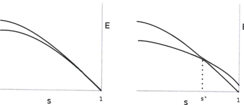
Figure 1-3: The two lowest energy levels near s = _{1 before (left) and after (right)}

adding the final penalty clause. A "perturbative cross" is created by adding this single clause which breaks the degeneracy between two local minima.

be important that these two satisfying assignments differ by a number of bit flips which is proportional to n. In

1181

we constructed a set of random instances where one of the satisfying assignnments is 000...0 and the other is 111...1. The Hamiltonian

H'(s) = (1 s_) 2 + sH'

has 2 energy levels which are close together as s -+ 1. The two lowest levels are

illustrated in Figure 1-3 (left). Suppose that for s near 1 the lower energy level corresponds to the bit string 000.. .0. The final step in constructing the problematic instance is to add a single clause which penalizes the lower level 000...0 but not 111...1. This "drags" the lower energy level above the upper one and creates the picture in Figure 1-3 (right). At s* there is an avoided cross and a very small gap which causes the adiabatic algorithm to fail. It turns out that the location of the avoided cross

s* approaches 1 as n -+ oo in this scenario, and one can use low order perturbation theory to compute its value. This type of avoided cross has been called a "perturbative cross". The nature of the ground state changes abruptly at s*. For s < s* most of the amplitude will be concentrated on bit strings with low Hamming weight whereas for

s > s* there is high amplitude only on states with Hamming weights close to n. It

is argued in

[4]

that problematic instances similar to this will occur with nonneglible probability in random ensembles of optimization problems and generically lead to the failure of the quantum adiabatic algorithm.

Young et al again numerically studied random instances of Exact Cover using Quantum Monte Carlo(641. The instances considered were chosen to have a unique satisfying assignment and ratio of clauses to bits near the phase transition. (There is a minor difference between the problem Hamiltonian Hp which was used here for each instance and that which was used in [631-see these references for details.) This time, instead of looking at the median minimum gap, they tried to look for instances where there appeared to be a sharp change in the ground state at some value of the

interpolating parameter s*. In order to diagnose such a sharp change, they computed (using quantum monte carlo) the "order parameter"

q = (ori )2

ni=1

at different values of s and observed that in some instances there is a value of s at which this order parameter changes abruptly. They found that the fraction of instances (out of 50 random instances considered at each value of n) where such an abrupt change occurs increases with n and may approach 1 for large n [64]. A recent paper of Neuhaus et. al has also reported abrupt changes in an order parameter for random instances of 3SAT [50]. We don't know if the sharp changes in the ground state observed by Young et al [64] (or the one observed by Neuhaus et al [50]) are associated with "perturbative crosses".

Performance on Random Regular Instances of XORSAT

In [21], Farhi et al showed that the quantum adiabatic algorithm can efficiently solve satisfiable instances of 2XORSAT on a ring. In this example the problem Hamiltonian to be minimized has nearest neighbor constraints on a line with periodic boundary conditions

H->

n+1i+

(1.12)

where each Ji,+ E

{±1}

and n+1 = o. This can be viewed as an instance of

2XORSAT since each term in the sum corresponds to a linear constraint on 2 variables of the form

zi G Zi+1 =

-Ji+1-The cost function 1.12 computes the number of violated clauses. We call this 2-regular 2XORSAT since the instance is defined on a 2 2-regular graph (a ring). For any choice of the couplings which is not frustrated-that is, when the final constraint on bits n and 1 is consistent with all other constraints , the Hamiltonian 1.4 with the above problem Hamiltonian is exactly solvable and the spectrum does not depend on the (consistent) couplings {Ji,+1} 1[21]. Every satisfiable instance has the same spectrum (and consequently the same eigenvalue gap) as the transverse field ising model described by the Hamiltonian 1.12 with each Jij+1 = 1. For the adiabatic

algorithm with beginning Hamiltonian

HB= (~~

and problem Hamiltonian 1.12 it is possible to exactly compute the minimum gap as a function of n and one obtains that it scales as an inverse polynomial in n [21].

Hamiltonians considered in [37] are of the form'

(1 - ch'1coci'c Jc)

C,2

each clause c is associated with 3 bits ii,ci 2,c, i3,c and a coupling Jc E {i1}. This problem Hamiltonian corresponds to an instance of 3XORSAT. The ensemble of in-stances was further restricted to those which are 3-regular (meaning that each bit is involved in exactly 3 clauses). Using the quantum cavity method (which we will discuss further in section 1.2.4 and in Chapter 5) and Quantum Monte Carlo, J6rg et al [37] have shown that there is a first order phase transition in this model at a critical value s ~ -. At this critical value properties of the ground state change abruptly; for example the transverse magnetization changes discontinuously.

J6rg et al also studied the ensemble of random instances of 3 regular 3 XORSAT which are restricted to have a unique satisfying assignment. A random choice of the couplings {Jc} and 3 regular hypergraph will produce an instance with a unique satisfying assignment with nonzero probability [371. For instances with a unique satisfying assignment, we can always apply a sequence of bit flip operators which map the unique solution to the bit string 000.. .0. Conjugating the problem Hamiltonian with this unitary transformation has the effect of replacing each Jc with the value

+1. So when restricted to instances with a unique satisfying assignment, the choice

of the couplings does not affect the spectrum (as in the case of 2 regular 2XORSAT [21] reviewed in the introduction). The 3 regular hypergraph which specifies the instance is therefore the only factor which determines the spectrum in this model. Using numerical diagonalization, the authors of [37] demonstrated that the quantum adiabatic algorithm does not succeed in polynomial time for random instances of this problem due to an exponentially small gap which occurs at s ~ . This agrees with the quantum cavity method and Quantum Monte Carlo results which apply to the random ensemble with no restrictions on the number of satisfying assignments.

In chapter 5 of this thesis we will demonstrate that the phase transition observed

by J6rg et al. [37] in random instances of 3-Regular 3XORSAT with a unique

satisfy-ing assignment occurs at exactly s =. In particular we show that there is a duality transformation which maps the problem Hamiltonian into the beginning Hamiltonian, and the beginning Hamiltonian into a problem Hamiltonian for a different instance (which occurs with equal weight in the ensemble). This demonstrates that the energy per spin, averaged over all instances, is symmetric about s = -. This implies that, if₂₁ there is a unique phase transition as a function of s, it can only occur at s

Note that although linear algebra solves 3XORSAT in polynomial time, heuristic algorithms such as the quantum adiabatic algorithm (which do not use linear algebra) presumably do not benefit from this fact. This is also true in the classical case-in reference [28] it was found numerically that the classical algorithm WALKSAT per-forms worse on random instances of 3-Regular 3XORSAT than on random instances

'We have rescaled the problem Hamiltonian and added an irrelevant constant in order to present the results of reference [37] in a consistent way with our notation.