en fr

(1)

HAL Id: hal-02126739

https://hal.archives-ouvertes.fr/hal-02126739

Submitted on 19 Nov 2019

HAL is a multi-disciplinary open access

archive for the deposit and dissemination of

sci-entific research documents, whether they are

pub-lished or not. The documents may come from

teaching and research institutions in France or

abroad, or from public or private research centers.

L’archive ouverte pluridisciplinaire HAL, est

destinée au dépôt et à la diffusion de documents

scientifiques de niveau recherche, publiés ou non,

émanant des établissements d’enseignement et de

recherche français ou étrangers, des laboratoires

publics ou privés.

SHREC’19 track: Feature Curve Extraction on Triangle

Meshes

E Moscoso Thompson, G Arvanitis, K Moustakas, N Hoang-Xuan, E R

Nguyen, M Tran, Thibault Lejemble, Loic Barthe, Nicolas Mellado, C

Romanengo, et al.

To cite this version:

E Moscoso Thompson, G Arvanitis, K Moustakas, N Hoang-Xuan, E R Nguyen, et al.. SHREC’19

track: Feature Curve Extraction on Triangle Meshes. 12th EG Workshop 3D Object Retrieval 2019,

May 2019, Gênes, Italy. pp.1 - 8. �hal-02126739�

(2)

S. Biasotti, G. Lavoué, B. Falcidieno, and I. Pratikakis (Editors)

SHREC’19 track: Feature Curve Extraction on Triangle Meshes

E. Moscoso Thompson†1 , G. Arvanitis2 , K. Moustakas2 , N. Hoang-Xuan4, E.R. Nguyen4, M. Tran4, T. Lejemble5, L. Barthe5, N. Mellado5 , C. Romanengo1,3, S. Biasotti1 , and B. Falcidieno1 .

1_{Istituto di Matematica Applicata e Tecnologie Informatiche ‘E. Magenes’ - CNR, Italy} 2_{Dept. of Electrical and Computer Engineering University of Patras, Rio, Patras, Greece}

3_{Dipartimento di Matematica, Università di Genova - UNIGE, Italy} 4_{Faculty of Information Technology, University of Science, VNU-HCM} 5_{IRIT, Université de Toulouse, CNRS, INPT, UPS, UT1C, UT2J, France}

Abstract

This paper presents the results of the SHREC’19 track: Feature curve extraction on triangle meshes. Given a model, the chal-lenge consists in automatically extracting a subset of the mesh vertices that jointly represent a feature curve. As an optional task, participants were requested to send also a similarity evaluation among the feature curves extracted. The various approaches presented by the participants are discussed, together with their results. The proposed methods highlight different points of view of the problem of feature curve extraction. It is interesting to see that it is possible to deal with this problem with good results, despite the different approaches.

CCS Concepts

• Information systems → Content analysis and feature selection; • Computing methodologies → Shape analysis; Search methodologies;

1. Introduction

The challenge of this SHREC’19 track is to extract feature curves from a set of models of different numbers of vertices and origins (scans or digital crafting). The models are represented by triangu-lations of various resolutions and vertex distributions. In the broad meaning of the word, a feature is an area of interest of the model. In the context of our track, a feature is intended as a bending of the surface that shapes a part of interest (e.g.: the eye of a statue is a feature, while the hand of a statue is not). A feature curve is a line that delineates a feature. In our contest we consider as a feature curve a set of vertices of the model that jointly define a contour, a valley or a ridge on the mesh. The mesh boundary (if it exists) is not considered a feature curve, as well as the noise artifacts (e.g., from scan inaccuracy and/or smoothing/resampling operations).

Feature curves drive the identification of features on a model and, in general, give local information about the surface. An effi-cient method for feature curves extraction, as intended in this track, needs to group sets of mesh vertices so that each set identifies a single feature curve.

The focus of this task is to find efficient methods for feature curve extraction that are able to highlight one or more subsets of vertices of the meshes in the track dataset. Moreover, as an

op-† Track Organizer

tional task, we asked the participants to submit a similarity evalua-tion among the feature curves extracted across all the models.

Therefore, the task proposed can be seen as a step towards the retrieval of features of interest on surfaces and, together with the previous SHREC tracks [BMea17], [MTW∗18] and [BMea18], it can help the automatic retrieval and recognition of style elements over art/cultural heritage data.

2. The dataset

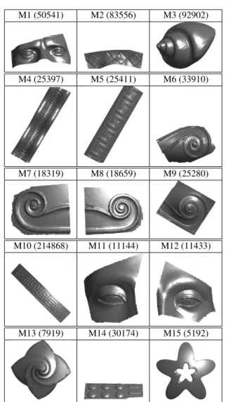
The dataset consists of 15 surfaces characterized by at least one feature curve. Some of the models are obtained through scans, while others are made in silico. Some mod-els are derived from the Visionair shape workbench (http: //visionair.ge.imati.cnr.it/) and the Turbosquid repository of 3D models (https://www.turbosquid.com/ Search/3D-Models). The original models of the ornaments from which we have derived the models from 4 to 10 are courtesy of the prof. Karina Rodriguez Echavarria. Both vertex distribution and density vary from mesh to mesh. Figure1shows an overview of the models, together with their number of vertices.

3. Groundtruth

The definition of a groundtruth for this task is a challenging job, since no formal definition of feature curve on surfaces exists.

(3)

2 E. Moscoso Thompson et. al. / SHREC’19 track: Feature Curve Extraction M1 (50541) M2 (83556) M3 (92902) M4 (25397) M5 (25411) M6 (33910) M7 (18319) M8 (18659) M9 (25280) M10 (214868) M11 (11144) M12 (11433) M13 (7919) M14 (30174) M15 (5192)

Figure 1: Overview of the dataset. In the brackets of each model is the corresponding number of vertices.

Feature curves derive from the human perception and interpre-tation of a surface, both in terms of localization and width. Psy-chologists and computer vision scientists who studied how humans perceive a shape have identified curvature variations, in terms of changes from convex to concave regions, as a key element of the human perception [PT96].

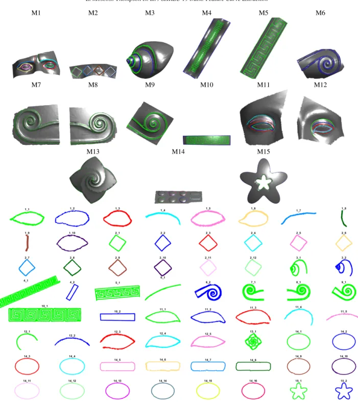
Keeping in mind this observations, the groundtruth has been defined by people from the IMATI-CNR (Italy) staff, requested to highlight the vertices of each model if, in their opinion, they were part of feature curves. Then, a groundtruth based on these individual annotations has been created. An overview of the final groundtruth is shown in Figure2.

For a given model M, the outcome of each method is expected to be a set of nMseparate lists f piof vertices, resembling the set of nM feature curves highlighted in the groundtruth. More formally, we expect a set of lists P(M) = { f p1, f p2, ...} for each M in the dataset. The evaluations are done by comparing this set with the

set GT (M) = { f c1, f c2, ..., f cnM} of feature curves defined in the

groundtruth. We consider two classifications:

• [Overall Comparison](O-comp): all the feature curves found on each model are jointly evaluated with the described evaluation measures, matching them with the groundtruth data. More for-mally, we compare the sets ∪if piand ∪if ci.

• [Curve-by-curve Comparison](CbC-comp): let us consider a feature curve f cjof the model M and the set P(M) of feature curves proposed by a participant. In the lists in P(M), we se-lected the closest to f ci and compare these two curves. The closest curve is selected by the same people that defined the groundtruth by voting the curve in P(M) which overlaps f cithe most.

The optional task was interpreted differently from the partici-pants. Two of them submitted a similarity matrix. The first provides a similarity measure among the models in the dataset, based on the distance among the feature curves identified; the second assesses similarity scores among single feature curves across the models. While it is hard to compare the results using numeric evaluations, some comparative remarks are drawn and discussed (Section6).

4. Participants

Six groups subscribed to this track and four sent their outcome. In the following we describe the methods submitted for evaluation.

4.1. Spectral based saliency estimation for the identification of features (SBSE) by G. Arvanitis and K. Moustakas This method is separated into two basic steps. At the first step, au-thors estimate the saliency of each vertex using spectral analysis. The magnitude of the estimated saliency identifies if a vertex is a feature or not. Based on the geometry, it is possible to say that the feature vertices represent the edge of a feature curve (both crests and valleys) or corners. At the second step, the mean curvature of the extracted features is estimated and it is used to classify the dif-ferent feature curves (if they exist). Additionally, the information related to the mean curvature and the saliency of each feature curve are used to find similarities with feature curves of other models. The execution time of the algorithm depends on: (i) the size of the mesh and (ii) the size of the patches, but generally, it is very fast. Definition and computation of vertex saliency

For each of the n vertex vi, a patch Pi= {vi, vi₁, . . . , vik} vertices

is created, which consists in the k geometrical nearest vertices to the vertex vibased on their coordinates (typically k = 15). These points are used to define a matrix Ni∈ R(k+1)×3for each vertex:

Ni= [ni, ni1, . . . , nik]

T

, ∀i = 1, . . . , n where the normal niof the vertex viis defined as:

ni= ∑ j∈Ni

ncj

|Ni| , ∀i = 1, . . . , n,

where ncj is the normal of the j-th face of the mesh and Ni is

(4)

M1 M2 M3 M4 M5 M6

M7 M8 M9 M10 M11 M12

M13 M14 M15

Figure 2: The final groundtruth of the contest. Top: the feature curves on the models; Bottom: feature curves represented one by one. Details are best appreciated in the digital version of this paper.

(5)

4 E. Moscoso Thompson et. al. / SHREC’19 track: Feature Curve Extraction

covariance matrix Ri= NTiNiis decomposed: eig(Ri) = UiΛi ∀i = 1, . . . , n where Ui∈ (R)3×3denotes the eigenvectors matrix and

Λi= diag(λi1, λi2, λi3)

The value siis the saliency of viand it is defined as the value given by the inverse norm − 2 of the corresponding eigenvalues:

si=_q 1 λ2_i1+ λ2_i2+ λ2_i3

, i= 1, . . . , n.

siis normalized to be in the [0, 1] range as follows: ¯

s= si− min(si)

max(si) − min(si), i= 1, . . . , n

Authors assume that a small value of saliency means that the vertex lies in a flat area, while a big value indicates that the vertex belong to an edge or corner. This characterization depends by the num-ber of dominant (or main) eigenvalues. For example, considering a cube, a vertex that "has" three, two or one dominant eigenvectors is, respectively, on a corner, on an edge or on a flat area.

A k-mean algorithm is used for separating the normalized values of the saliency into five different classes. The first two are con-sidered as non-feature vertices, while the other are actual feature vertices.

Clustering of salient vertices

The feature curves are identified by grouping the feature vertices based on mean curvature mcvalues. Since the initial number of the feature curves is unknown for each model, the optimal number of cluster is supposed to range from 1 to 5 and it is estimated using the Calinsky-Harabasz clustering evaluation criterion, followed by the k-means algorithm that performs the actual clustering.

Moreover, feature curve similarities between different models is assessed through the histograms of saliency and mean curvature. More specifically, for a given model the histograms of the ¯svalue and the normalized mean curvature are computed (respectively ˙s∈ R10×1and ˙m∈ R10×1). Then they are horizontally stacked in the vector q = [ ˙s, ˙m]. The correlation coefficient r of two models A and B defined by the vectors qAand qBis:

r= 20 ∑ i=1 (qAi− ¯qA)(qBi− ¯qb) s ( 20 ∑ i=1 (qAi− ¯qA))( 20 ∑ i=1 (qBi− ¯qb))

where ¯q∗ represents the mean value. The lower r is, the higher is the similarity between A and B.

4.2. Point aggregation based on angle and curvature saliency (PCs) by Nhat Hoang-Xuan, E-Ro Nguyen, Minh-Triet Tran

These participants propose two methods, labelled PCs:A and PCs:C. Both have the same approach: defining a set of candidate vertices with a significant difference in a given property. Then can-didate vertices that might be on a flat region and/or small fragments

are removed, to reduce noise in the output. With this approach, all the feature curves obtained on a single model are grouped, thus we consider these methods only in the overall comparison. The core difference between the two methods is how the candidate vertices are determined.

Angle-based vertex saliency (PCs:A)

The first method works in three steps. First, the angle θibetween each pair of connected triangles (by one edge) is computed. Then, if θi> αmeani(θi) (with mean equal to the average value), the two extremes of the relative edge are considered as candidate vertices. α is set equal to 1.3 in most cases, aside from 1.6 for Model2 and 2.6 for Model3. Second, if two candidate vertices share an edge larger than the double average length of the edges the two candidate vertices are removed. Finally, a graph with each pair of candidate vertices as nodes is created. All the connected components of this graph are computed and, if the number of vertices in a component is less than 1% of the number of vertices of the mesh, the vertices are removed.

Normal curvature-based vertex salicency (PCs:C)

The second method runs in three steps. First, the oriented normals per-triangle are computed and for each vertex the normal of a ver-tex is the average of the weighted sum of its incident faces, with weights being proportional to a face’s area. For each edge in the mesh, if its extremes are p1, p2with normals n1, n2, an estimation of its curvature is given by:

curv=(n2− n1)(p2− p1) |p2− p1|2

Second, the average curvature of each vertex viis estimated as the geometric mean of the absolute values of all the edge curvatures of incident edges at the selected vertex. This evaluation is smoothed by averaging the value with those of its immediate neighbors. This is repeated multiple times. Vertices with large touching triangles indicate that the surrounding area is relatively flat and thus filtered away, checking if their adjacent vertices have length larger than some value proportional to the average of the edge length. Of the remaining vertices, those that have a curvature value larger than a+ k(meani(curv(vi))) are flagged as possible elements of some feature curves. This formulation derives from the following obser-vation: if the curvature value is larger than the average, at some point then it is highly possible that it is part of some curve, but in a sample with mostly noisy texture, this limit needs to be relaxed. In this method, a = 0.025 and k = 0.7. Finally, to reduce noise, the components with less than 5 vertices are removed. Also, large com-ponents that have no nearby other flagged vertices are removed.

4.3. Point-based multi-scale curve voting (PMCV) by T. Lejemble, L. Barthe and N. Mellado

This method extracts feature lines from meshes using a voting sys-tem based on a set of 3D curves generated in the direction of mini-mal curvature in anisotropic regions.

(6)

Point cloud sampling and curve generation

Each mesh M is converted to a dense point cloud with a uniform point cloud P through a uniform sampling weighted by the face area. The authors of the methods observe that feature curves as in-tended in this track are characterized by a small curvature along the feature and a large curvature in orthogonal direction. The curvature is evaluated using a local surface estimation called APSS [GG07]. Curves are generated at five levels of scale, based on the size of the neighbor used to approximate the surface with APPS, namely ti= ₂e¯(2 + i ¯e), i = 0, . . . , 4 where ¯eis the median edge lengths in M. P is sub-sampled in 5 sparse point clouds Piusing a Poisson disk sampling, with radius ri=10ti plus an additional cloud Pl, with rl=t20. For each ti, curves are iteratively generated from each point in Plas follows:

pj+1= pro j(pj+ 4v(pj)) with 4 =t0

2. v(pj) is the direction of minimal principal curvature computed on Pi. pro j projects a point on the APPS surface approx-imation of Pi, ensuring that the curve remains close to the surface. The iterations stop after reaching a maximum, set at 105, or if the curve leaves the curved area, i.e. if||κ1|−Ki|

Ki > α, where κ1is the

maximal curvature, Kiis set to the 90thcentile of maximal curva-ture absolute values calculated in Plat scale tiand α is set to 0.5. In order to filter noise or insignificant features, if the number of iterations is lower than 50, the curve is discarded.

Voting-based feature line extraction

The vertices of M accumulate votes from the extracted neighbor curves. Each vertex of each curve accumulates a vote in its neigh-boring mesh vertices. The size of the spherical neighborhood is ¯e. A vote is a negative scalar coefficient for valley lines and positive for crest lines, with absolute values ranging from 0 to 1 accord-ing to the distance between the curve vertex and the mesh vertex. Sign is used to balance the sum of vertices close to both valley and crests. Finally, a region growing process delineates individual set of vertices based on these votes. A region grows from a vertex to its neighbor if the sum of the votes has the same sign and if its absolute value is greater than ₂₀1Vmax, where Vmaxis the maximal absolute value of votes on the vertices of the mesh.

4.4. Feature curve characterization via mean curvature and algebraic curve recognition via Hough transforms (MHT) by C. Romanengo, S. Biasotti and B. Falcidieno

This feature curve recognition method derives from the technique described in [TBF18] and works in three steps.

Feature point characterization

Authors evaluate the mean curvature values in the mesh vertices to detect the feature points adopting the curvature estimation based on normal cycles [CSM03] implemented in the Toolbox graph [Pey]. The vertices at which the mean curvature is significant (e.g with high maximal and low minimal curvature values) are selected as feature points. This is automatically achieved by filtering the distri-bution of the mean curvature by means of two filtering thresholds mand M. Note that m and M are two input parameters. Their value

varies according to the precision threshold set for the property used to extract the feature points (e.g., in our case, two typical values of mand M are 15% and 85%, respectively).

Feature curve aggregation

Feature points are aggregated to determine the elements that po-tentially correspond to a curve. Once detected, the set of feature points is subdivided into smaller clusters (that is, groups of points sharing some similar properties) by using a clustering algorithm. The Density-Based Spatial Clustering of Applications with Noise (DBSCAN) method [EKSX96], is adopted which groups together points that lie close by marking as outliers isolated points in low-density regions. The DBSCAN algorithm requires two parameters: a threshold used as the radius of the density region, and a positive integer that represents the minimum number of points required to form a dense region. As feature curves, the output of the DBSCAN algorithm is submitted. To estimate the density of the feature points and, therefore, the minimum number of points in a region, the K-Nearest Neighbor(KNN) [FBF77] is used. In general, the K value of the KNN search is set to 15 for MHT1 and to 4 for MHT2. Curve approximation using Hough transforms

Finally, the feature curves are fitted with template curves to recog-nize their type and quantify the parameters characterizing such a feature. This step is obtained following the procedure based on the Hough transform described in [TBF18]. In this contest, the follow-ing dictionary of curves is considered: circles, Lamet curve, citrus curve, geometric petal and Archimedean spiral, see [TBF18] for details. In general, combinations or additional families of curves are possible [Shi95]. The peculiarity of the Hough transform is to estimate in a family of curves, the parameters of the curve a = (a1, . . . , an) that better fits a given set of points. The curves considered have at most one or two parameters. Depending on the curve, these parameters estimate its bounding box, diagonal, radius, etc.

The distance between the two curves C1 and C2 is defined as the norm L1of the parameters corresponding to these curves, i.e., d(C1, C2) = |aC1, aC2|1, where aC1 and aC2 are the parameters of

the curves C1and C2, respectively. Note that such a notion of dis-tance assumes the curve parameters are homogeneous in terms of the properties measured; this implies that the distance between two feature curves is computed only if they belong to the same family.

5. Evaluation Measures

Apart of the well-known Hausdorff distance between two sets of points, there is not a standard measure for the evaluation of this kind of tasks. Also, notice that despite being curves, our groundtruth is defined by sets of points that are not sorted, thus distances for ordered polylines like the Fréchet distance are not suitable [EGHP∗02]. We used the the Direct Hausdorff distance [DD09], the Dice coefficient [TH15] and the Jaccard index [TH15]. More precisely:

• The Direct Hausdorff distance from the points a ∈ A ⊂ R3_{to the} points b ∈ B ⊂ R3is defined as follows:

(7)

with d the euclidean distance. As a reference, the well known Hausdorff distancebetween A and B is

max{ddHaus(A, B), ddHaus(B, A)}

In order to have coherent evaluation through different models, we make this measurement on resized models so that their loads are as close as possible.

• The Dice coefficient between two sets (let them be S and R) is defined as

dice(S, R) = 2|S ∩ R| |S| + |R|,

where | · | denotes the number of elements. It ranges from 0 (no match), to 1 (perfect match).

• The Jaccard index is defined as:

jaccard(S, R) = dice(S, R) 2 − dice(S, R), that varies from 0 to 1, the higher the better.

The Direct Hausdorff distance score is used to evaluate how well the overall shape of the curves extracted by the participants fit the groundtruth and vice-versa. The other two measures are used to evaluate the precision of the methods. While a score of 1 is not mandatory for a method to be considered good, the higher the value is, the better the extracted curve fits its groundtruth counterpart. After running our measures, we saw that the Jaccard index and the Dice coefficient scores on the participants’ results are different in terms of scale but equivalent in terms of classification of the method performances. Thus, we decided to report only the Dice coefficient, for brevity.

6. Results and discussions

A total of six runs was submitted for evaluation. The authors of the SBSE and MHT* methods sent results for both the mandatory and the optional task. The authors of the PMCV and PCs methods sub-mitted only the mandatory task. Moreover, the PCs results report an unique feature curve per model so they are considered in the overall comparisononly.

The results for both classifications (curve-by-curve and overall) are reported in Table1and Table2.

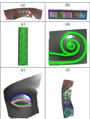
The participants face this track with different approaches that often have been tailored for more general projects. Depending on the design choices, the results vary in precision, sensitiveness and overall quality. Our quantitative evaluations provide an interpreta-tion of these methods for this specific contest and are not meant to evaluate the absolute quality of the methods. Indeed, none method stands out in general; depending on the different application/needs, the methods present their own peculiarities and answer the chal-lenge more or less properly. If interested in the strongest features (in terms of bending) of a model, SBSE provides a quick over-all preview of the related feature curves, quite robust to noise. As shown in Figure3(a), SBSE is able to extract the jointed feature curves even in presence of acquisition noise, with good precision. PMCV has impressive precision in its extraction process. Such a precision could be ideal to identify different features that share a jointed feature curve. Figure3(b) shows how this method is able

O-comp- ddHausfrom GT to Parts

Model SBSE PCs:A PCs:C PMCV MHT1 MHT2 M1 0.068 0.054 0.105 0.675 1.570 1.570 M2 0.054 0.060 0.032 0.079 0.071 0.060 M3 0.074 0.006 0.005 0.001 0.048 0.048 M4 3.047 3.694 2.771 0.162 3.555 3.555 M5 0.887 1.019 2.100 0.921 1.019 1.019 M6 1.229 0.033 1.049 2.246 0.650 0.089 M7 0.018 0.010 0.028 0.016 0.012 0.012 M8 0.062 0.006 0.027 0.037 0.011 0.011 M9 1.622 0.165 1.699 1.716 0.081 0.081 M10 2.427 0.003 0.582 2.348 4.585 4.585 M11 0.091 0.009 0.035 0.013 0.045 0.045 M12 0.062 0.036 0.064 0.011 0.040 0.010 M13 0.035 0.057 0.023 0.070 0.013 0.013 M14 0.024 0.004 0.027 0.004 0.010 0.010 M15 0.004 0.009 0.077 0.145 0.030 0.030

O-comp- ddHausfrom Parts to GT

O-comp- Dice coefficient

Table 1: The evaluation measures of the O-comp classification. The ddHausdistance measure is computed from groundtruth (GT) to the feature curve proposed by the participants (Parts) and vice-versa. The lower its score is (0 at best), the better. For the Dice coefficient, the higher the score is (1 at best), the bettee. Refer to Figure2to see which model is evaluated in each cell. Bests results are highlighted with bold font.

to separate the L-shaped bumps of the mesh with different feature curves. It usually detects more feature curves than those selected in the groundtruth. The main reason is that this method extracts the set of valley and crest lines in the mathematical sense, while the groundtruth focuses on a user-specified subset. It may also happen that the 3D curves generation stops at non anisotropic areas such as corners. In that case, a feature line is separated in several curves. The feature lines provided by the PMCV are generally thicker than those in the groundtruth. If required, thinner set of lines can be ob-tained by reducing the distance used for the curve voting, although representative features could be discarded in this way. About the

(8)

CbC-comp- ddHausfrom GT to Parts FC id. SBSE PMCV MHT1 MHT2 1_1 0.604 0.014 0.013 0.013 1_2 0.601 0.036 0.034 0.034 1_3 0.575 0.084 0.039 0.039 1_4 n.c. 0.041 0.064 0.064 1_5 0.555 0.056 0.035 0.035 1_6 0.527 0.128 0.050 0.050 1_7 0.541 0.027 0.028 0.028 1_8 n.c. < 0.001 n.c. n.c. 1_10 0.547 0.035 0.024 0.024 2_1 0.673 0.005 0.674 0.016 2_2 0.467 0.005 0.468 0.013 2_3 0.461 0.013 0.461 0.015 2_4 0.681 0.003 0.681 0.019 2_5 0.686 0.002 0.688 0.019 2_6 0.473 0.002 0.475 0.018 2_7 0.461 0.004 0.462 0.017 2_8 0.475 0.005 0.476 0.022 2_9 0.453 0.002 0.454 0.017 2_10 0.674 0.002 0.674 0.018 2_11 0.686 < 0.001 0.686 0.022 2_12 0.683 0.003 0.685 0.016 3_1 n.c. 0.092 n.c. n.c. 3_2 0.414 0.007 0.062 0.062 4_1 0.048 0.005 0.036 0.036 4_2 0.124 0.027 n.c. n.c. 5_1 0.021 < 0.001 0.102 0.102 6_1 n.c. 0.005 n.c. 0.561 6_2 0.053 0.006 1.021 1.021 7_1 0.012 0.007 0.010 0.010 8_1 0.012 0.007 0.017 0.017 9_1 2.459 0.005 0.016 0.016 10_1 5.031 0.001 0.019 0.019 10_2 3.192 0.285 n.c. n.c. 11_1 0.102 0.035 0.033 0.033 11_2 0.028 0.062 0.048 0.048 11_3 n.c. 0.011 0.011 0.011 11_4 0.171 0.039 0.014 0.014 11_5 n.c. 0.005 0.005 0.005 12_1 0.137 0.083 0.065 0.143 12_2 n.c. 0.006 0.005 0.155 12_3 n.c. 0.023 0.004 0.078 12_4 0.027 0.051 0.029 0.029 12_5 0.082 0.026 0.031 0.097 13_1 < 0.001 0.022 0.067 0.067 14_1 0.716 0.006 < 0.001 < 0.001 14_2 0.464 0.006 0.011 0.011 14_3 0.464 0.007 < 0.001 < 0.001 14_4 0.470 0.007 0.006 0.006 14_5 0.672 0.008 0.006 0.006 14_6 0.654 0.007 0.015 0.015 14_7 0.655 0.007 0.008 0.008 14_8 0.667 0.006 0.008 0.008 14_9 0.721 0.007 0.012 0.012 14_10 0.703 0.007 < 0.001 < 0.001 14_11 0.708 0.007 0.003 0.003 14_12 0.500 0.007 0.012 0.012 14_13 0.494 0.007 0.011 0.011 14_14 0.513 0.007 < 0.001 < 0.001 14_15 0.519 0.007 0.004 0.004 14_16 0.470 0.006 0.009 0.009 15_1 0.260 n.c. 0.009 0.009 15_2 0.151 0.022 0.007 0.007

CbC-comp- ddHausfrom Parts to GT

FC id. SBSE PMCV MHT1 MHT2 1_1 0.035 0.006 0.006 0.006 1_2 0.016 0.006 0.006 0.006 1_3 0.052 0.021 0.110 0.110 1_4 n.c. 0.021 0.020 0.020 1_5 0.031 0.006 0.006 0.006 1_6 0.057 0.113 0.118 0.118 1_7 0.083 0.020 0.062 0.062 1_8 n.c. 0.049 n.c. n.c. 1_10 0.028 0.082 0.081 0.081 2_1 0.011 0.171 0.012 0.012 2_2 0.006 0.081 0.004 0.003 2_3 0.006 0.004 0.007 0.014 2_4 0.005 0.118 0.004 0.004 2_5 0.018 0.155 0.018 0.017 2_6 0.010 0.127 0.017 0.016 2_7 0.015 0.166 0.015 0.017 2_8 0.013 0.146 0.017 0.018 2_9 0.016 0.169 0.017 0.016 2_10 0.015 0.185 0.020 0.018 2_11 0.011 0.146 0.017 0.017 2_12 0.004 0.131 0.005 0.005 3_1 n.c. 0.172 n.c. n.c. 3_2 0.035 0.097 0.016 0.016 4_1 0.023 0.313 0.035 0.035 4_2 0.092 0.005 n.c. n.c. 5_1 0.887 0.470 1.086 1.086 6_1 n.c. 0.079 n.c. 0.008 6_2 0.060 0.279 1.213 1.213 7_1 0.070 0.220 0.048 0.048 8_1 0.064 0.314 0.046 0.046 9_1 1.638 0.228 0.071 0.071 10_1 0.108 0.150 0.049 0.049 10_2 2.427 13.239 n.c. n.c. 11_1 0.007 < 0.001 0.005 0.005 11_2 0.018 0.008 0.011 0.011 11_3 n.c. 0.013 0.015 0.136 11_4 0.091 0.009 0.062 0.062 11_5 n.c. 0.028 0.006 0.006 12_1 0.064 0.005 0.040 0.006 12_2 n.c. 0.008 0.069 0.008 12_3 n.c. 0.011 0.019 0.016 12_4 0.006 0.005 0.007 0.007 12_5 0.005 < 0.001 0.004 0.006 13_1 0.035 0.076 0.013 0.013 14_1 0.002 < 0.001 0.003 0.003 14_2 < 0.001 < 0.001 0.004 0.004 14_3 0.003 < 0.001 0.003 0.003 14_4 0.004 < 0.001 0.004 0.004 14_5 0.023 0.003 0.004 0.004 14_6 0.007 0.004 0.004 0.004 14_7 0.011 < 0.001 0.010 0.010 14_8 0.024 < 0.001 0.069 0.069 14_9 0.004 < 0.001 0.002 0.002 14_10 0.004 < 0.001 0.006 0.006 14_11 0.004 < 0.001 0.004 0.004 14_12 0.004 0.003 0.002 0.002 14_13 0.004 < 0.001 0.004 0.004 14_14 0.003 < 0.001 0.004 0.004 14_15 0.004 0.003 0.002 0.002 14_16 0.004 0.004 0.004 0.004 15_1 0.010 n.c. 0.030 0.030 15_2 0.010 < 0.001 0.013 0.013

CbC-comp- Dice coefficient Mod SBSE PMCV MHT1 MHT2 1_1 0.121 0.650 0.636 0.636 1_2 0.145 0.450 0.413 0.413 1_3 0.244 0.435 0.503 0.503 1_4 n.c. 0.499 0.445 0.445 1_5 0.180 0.434 0.578 0.578 1_6 0.214 0.458 0.481 0.481 1_7 0.041 0.382 0.338 0.338 1_8 n.c. 0.447 n.c. n.c. 1_10 0.126 0.354 0.334 0.334 2_1 0.094 0.296 0.025 0.048 2_2 0.194 0.542 0.147 0.449 2_3 0.164 0.633 0.119 0.332 2_4 0.265 0.457 0.176 0.461 2_5 0.060 0.102 0.033 0.082 2_6 0.077 0.537 0.009 0.029 2_7 0.041 0.076 0.016 0.035 2_8 0.062 0.337 0.018 0.044 2_9 0.029 0.339 0.015 0.019 2_10 0.104 0.032 0.022 0.038 2_11 0.078 0.248 0.037 0.044 2_12 0.174 0.474 0.107 0.282 3_1 n.c. 0.443 n.c. n.c. 3_2 0.586 0.487 0.497 0.497 4_1 0.300 0.126 0.426 0.426 4_2 0.159 0.590 n.c. n.c. 5_1 0.381 0.304 0.414 0.414 6_1 n.c. 0.663 n.c. 0.046 6_2 0.318 0.357 0.516 0.516 7_1 0.333 0.479 0.528 0.528 8_1 0.313 0.454 0.533 0.533 9_1 0.218 0.270 0.390 0.390 10_1 0.331 0.394 0.311 0.311 10_2 0.131 0.433 n.c. n.c. 11_1 0.497 0.627 0.680 0.680 11_2 0.367 0.393 0.404 0.404 11_3 n.c. 0.546 0.553 0.553 11_4 0.043 0.511 0.489 0.489 11_5 n.c. 0.778 0.705 0.705 12_1 0.190 0.588 0.535 0.230 12_2 n.c. 0.817 0.713 0.131 12_3 n.c. 0.137 0.286 0.237 12_4 0.553 0.572 0.514 0.514 12_5 0.557 0.766 0.774 0.450 13_1 0.574 0.567 0.976 0.976 14_1 0.227 0.559 0.979 0.979 14_2 0.224 0.529 0.987 0.987 14_3 0.219 0.509 0.978 0.978 14_4 0.002 0.450 0.942 0.942 14_5 0.001 0.489 0.795 0.795 14_6 0.027 0.657 0.646 0.646 14_7 0.178 0.655 0.739 0.739 14_8 0.153 0.576 0.667 0.667 14_9 0.002 0.478 0.897 0.897 14_10 0.227 0.516 0.919 0.919 14_11 0.004 0.465 0.952 0.952 14_12 < 0.001 0.446 0.956 0.956 14_13 0.226 0.510 0.954 0.954 14_14 0.225 0.465 0.983 0.983 14_15 < 0.001 0.464 0.980 0.980 14_16 0.002 0.466 0.907 0.907 15_1 0.512 n.c. 0.913 0.913 15_2 0.732 0.662 0.921 0.921

Table 2: The evaluation measures of the CbC-comp classification. The ddHausdistance measure is computed from groundtruth (GT) to the feature curve proposed by the participants (Parts) and vice-versa. The lower its score is (0 at best), the better. For the Dice coefficient, the higher the score is (1 at best), the bettee. Refer to Figure2to see which model is evaluated in each cell. Model1_9 and is not reported since no one was able to detect it. Bests results are highlighted with bold font.

PCs runs, while they do not separate the feature vertices in differ-ent feature curves, they almost always provide a super-set of the vertices of the groundtruth jointed feature curves. Also, as shown in Figure3(c,d), the methods are very precise in case of very sharp features, as those in Models 5 and 9. A good balance between pre-cision and vertex clustering is obtained by MHT, which recognizes most of the expected feature curves, balancing the number of

ver-tices recognized and the curve fragmentation (with respect to our groundtruth). An example of this is shown in Figure3(e,f).

For the optional task, SBSE provides a global distance between two models based on histogram-based feature vectors. For exam-ple, M4 and M10 are considered similar based on this evaluation, as well as M11 and M12, M7 and M8, M6 and M9. Another way to approach the problem of similarity is that of MHT, which provides

(9)

a similarity measure among the single feature curves, even those in the same model. In other words, it performs a local similarity evalu-ation of the models. The similarity evaluevalu-ation is doable with curves that are obtained using the same family of curves. For instance, the eyes in Model 11 and 12 are mutually considered similar, as well as each pair of rings on Model 14. An example of curves sorted by similarity in a single family is shown in Figure4.

As a final remark, the participants show different views for the problem of feature curve extraction: the main contrast between the feature curves proposed by the participants and those in the groundtruth is due to its definition, being it influenced by the hu-man perception. Despite this, the proposed methods highlight that such a problem could be automatized in future with more efforts in this research path.

(a) (b)

(c) (d)

(e) (f)

Figure 3: An example of the the results from SBSE (a), PMCV (b), PCs:A (c), PCs:C (d), MHT1 (e) and MHT2 (f).

7. Acknowledgment

This study was partially supported by the CNR-IMATI projects DIT.AD004.028.001 and DIT.AD021.080.001.

References

[BMea17] BIASOTTIS., MOSCOSOTHOMPSONE.,ET AL.: Retrieval of Surfaces with Similar Relief Patterns. In Eurographics Workshop on 3D Object Retrieval(2017), Pratikakis I., Dupont F., Ovsjanikov M., (Eds.), The Eurographics Association.1

[BMea18] BIASOTTIS., MOSCOSOTHOMPSONE.,ET AL: SHREC’18 track: Recognition of geometric patterns over 3D models. In Eurograph-ics Workshop on 3D Object Retrieval(2018), The Eurographics Associ-ation.1

M6 M8 M7 M9

Figure 4: Based on MHT similarity evaluation, the most similar feature curves to the feature curve extracted on Model 6 (red). From the second images, from left to right, the extracted feature curves on other models (reported in the brackets) from closest to farthest, are shown.

[CSM03] COHEN-STEINERD., MORVAN J.-M.: Restricted Delaunay triangulations and normal cycle. In Proc. of the 9th_{Ann. Symp. on}

Computational Geometry(New York, NY, USA, 2003), SCG ’03, ACM, pp. 312–321.5

[DD09] DEZAM. M., DEZAE.: Encyclopedia of Distances. Springer Berlin Heidelberg, 2009.5

[EGHP∗02] EFRAT, GUIBAS, HAR-PELED S., MITCHELL, MURALI: New similarity measures between polylines with applications to mor-phing and polygon sweeping. Discrete & Computational Geometry 28, 4 (Nov 2002), 535–569.5

[EKSX96] ESTERM., KRIEGELH. P., SANDERJ., XUX.: A density-based algorithm for discovering clusters in large spatial databases with noise. In 2nd_{Int. Conf. Knowledge Discovery and Data Mining}_(1996),

AAAI Press, pp. 226–231.5

[FBF77] FRIEDMANJ. H., BENTLEYJ. L., FINKELR. A.: An algo-rithm for finding best matches in logaalgo-rithmic expected time. ACM Trans. Math. Softw. 3, 3 (Sept. 1977), 209–226.5

[GG07] GUENNEBAUDG., GROSS M.: Algebraic point set surfaces. ACM Trans. Graph. 26(07 2007), 23.5

[MTW∗_18] _M_OSCOSO _T_HOMPSON _{E., T}_ORTORICI _{C., W}_ERGHI _N.,

BERRETTIS., VELASCO-FOREROS., BIASOTTIS.: Retrieval of Gray Patterns Depicted on 3D Models. In Eurographics Workshop on 3D Ob-ject Retrieval(2018), Telea A., Theoharis T., Veltkamp R., (Eds.), The Eurographics Association.1

[Pey] PEYRE G.: Toolbox graph - A tool-box to process graph and triangulated meshes. http://www.ceremade.dauphine.fr/∼peyre/matlab/graph/content.html.5 [PT96] PHILLIPSF., TODDJ. T.: Perception of local three-dimensional shape. Journal of experimental psychology. Human perception and per-formance 22 4(1996), 930–44.2

[Shi95] SHIKINE. V.: Handbook and atlas of curves. CRC, 1995.5 [TBF18] TORRENTEM.-L., BIASOTTIS., FALCIDIENOB.:

Recogni-tion of feature curves on 3D shapes using an algebraic approach to hough transforms. Pattern Recognition 73 (2018), 111 – 130.5

[TH15] TAHAA. A., HANBURYA.: Metrics for evaluating 3D medi-cal image segmentation: analysis, selection, and tool. In BMC Medimedi-cal Imaging(2015).5