HAL Id: hal-01899462
https://hal.archives-ouvertes.fr/hal-01899462
Submitted on 19 Oct 2018
HAL is a multi-disciplinary open access archive for the deposit and dissemination of sci-entific research documents, whether they are pub-lished or not. The documents may come from teaching and research institutions in France or abroad, or from public or private research centers.
L’archive ouverte pluridisciplinaire HAL, est destinée au dépôt et à la diffusion de documents scientifiques de niveau recherche, publiés ou non, émanant des établissements d’enseignement et de recherche français ou étrangers, des laboratoires publics ou privés.
M. Lavagna
To cite this version:
M. Lavagna. Transport through an interacting quantum dot driven out-of-equilibrium. Jour-nal of Physics: Conference Series, IOP Publishing, 2015, 592, pp.012141. �10.1088/1742-6596/592/1/012141�. �hal-01899462�
Transport through an interacting quantum dot
driven out-of-equilibrium
Mireille Lavagna*
Universit´e Grenoble Alpes, CEA, INAC-SPSMS, Grenoble, France E-mail: [email protected]
Abstract. We study a single-level quantum dot in the presence of strong Coulomb interaction under nonequilibrium condition. By extending the equation of motion method to nonequilibrium, we study the transport behavior of the system when a dc bias voltage is applied to the leads. The spectral density exhibits two broad peaks centered around the normalized dot level energies and a split Kondo resonance at low temperature with two peaks pinned at the Fermi level of each lead. The approach allows one to recover the unitary condition for the density of states at the Fermi levels and by the way to cure the long-standing problem about the presence of spurious peak in the density of states at equilibrium. Finally we discuss the consequences for the linear and di↵erential conductances of the quantum dot in its steady state.
1. Introduction
Understanding the mechanisms involved in interacting systems far from equilibrium is one of the major problems in condensed matter physics. We study in this paper quantum dots under nonequilibrium conditions. Quantum dots are realized by confining electrons in a small spatial region weakly coupled to two leads. They give rise to a Kondo e↵ect at low temperature [1] when the dot is occupied by a single electron, and hence acquires a spin which is antiferromagnetically coupled to the spin of the conduction electrons in the leads. Predicted at a theoretical level at the end of the 80ies [2, 3], the Kondo e↵ect in quantum dots has been observed experimentally since the end of the 90ies [4-6]. Out of equilibrium the Kondo e↵ect in quantum dots has been studied by a variety of analytical and numerical techniques. In most cases, these techniques combine many-body methods to treat strong interactions with non-equilibrium Green function techniques to take non-equilibrium conditions into account. The system is driven out of equilibrium either by the application of a dc bias voltage between the two leads or by irradiation with an electromagnetic field. Driving the system out of equilibrium leads to a decoherence of the Kondo many-body singlet state and induces a crossover from the Fermi liquid strong coupling regime (local Fermi liquid) to the weak coupling regime. Despite all the e↵ort developed these last years along this direction, many open questions remain about how electron correlations and nonequilibrium e↵ects interfere in those mesoscopic systems.
In this paper we present how the equation of motion (EOM) technique can be generalized to the study of quantum dots out of equilibrium when a dc bias voltage is applied to the two leads. The EOM technique had been applied to the original Anderson model in equilibrium a long time ago [7-9] in the context of dilute magnetic alloys and later on in that of quantum dots [10-20]. The strength of the method is to allow the description of both the high temperature regime
with logarithmic dependence of either resistivity for dilute alloys (or conductance for quantum dots respectively) and the low temperature regime with the formation of a Kondo resonance in the spectral density in addition to broad peaks. However the method is known to present some serious drawbacks as the presence of a spurious peak in the density of states at low temperature. This spurious peak corresponds to an antiresonance in the density of states which occurs just at the position of the Kondo resonance peak at the particle-hole symmetric limit, letting the Kondo physics paradoxically not recovered in that limit. By carefully extending the EOM method to nonequilibrium, it turns out that we solved this long-standing problem and cure the presence of this spurious peak in the spectral density at equilibrium.
The organization of the paper is the following. In section 2 we present the results for the retarded electronic Green function in the dot obtained by solving the set of equations of motion of successive order Green functions when truncated at the second order in t↵ by performing all
possible decouplings preserving the spin: hn i, hc†k0↵¯ck↵¯i, and the mixed parameter hf¯†ck↵¯i.
In section 3 we show how, provided that the system is in its steady state, the various decoupling parameters considered can be determined self-consistently from the knowledge of the retarded dot Green function only, even if the fluctuation-dissipation theorem does not hold any longer when the system is out of equilibrium. The derivation is exact and does not require the use of any ansatz as was often used in the past. In Section 4 we stress the importance of incorporating the normalization of the dot level energy and of the inverse lifetime broadening of the various excited states involved in the expression of the retarded dot Green function. The former corrections correspond to the dressing of the bare propagators by interactions and are obtained by taking the real part of the self energy term, whereas the latter corrections are evaluated by means of the generalized Fermi golden rules. In section 5 we discuss the results for the spectral density and the linear and di↵erential conductances when the system driven out of equilibrium is in its steady state.
2. Equation of motion approach for the Anderson model out-of-equilibrium
We consider a quantum dot with two leads driven out of equilibrium by the e↵ect of a finite bias voltage V and if appropriate placed in a magnetic field B. We model the quantum dot by the single-level Anderson model [21]
H = X k,↵2(L,R), "k↵ c†k↵ ck↵ + X " f†f + U n"n#+ X k,↵2(L,R), (t↵ c†k↵ f + h.c.). (1)
where c†k↵ (ck↵ ) creates (destroys) an electron in the ↵ (left and right) lead with momentum
k, spin ( = ±1) and energy "k↵ ; the equilibrium momentum distribution in the ↵ lead is
nF(! µ↵) = [exp[(! µ↵)/kBT )] + 1] 1 where µ↵ is the chemical potential in the ↵ lead and
eV = µL µR the bias voltage applied between the two leads; f† (f ) creates (destroys) an
electron in the dot with energy " = "0+ /2, where = µBB is the Zeeman splitting due to
the magnetic field B; n = f†f ; U is the on-site Coulomb interaction -charging energy- in the dot; and t↵ is the tunneling matrix element between the states|k↵ i and | i in the leads and
the dot respectively.
The equation of motion technique has been extensively used in the past to study quantum impurities at equilibrium. More recently there have been works to extend its applicability to nonequilibrium [10-20]. Briefly speaking the equation of motion method consists in di↵erentiating the Green function Gr(t, t0) with respect to time t, thereby generating higher-order Green’s functions. Writing the equations of motion for those series of Green-functions leads to a set of linear equations that can be closed -truncated- at a given order by performing the proper decouplings. Using the set of EOM truncated at the second order in t↵ by performing a
decoupling in terms of all possible two-operator correlation functions with equal-spin,hf¯†c↵k¯i,
hc†↵k0¯c↵k¯i and hn i, we obtain the following expression for Gr(!) [20] Gr(!) = 1 hn¯i ! " ⌃0(!) ⇧ 1(!) + hn¯i ! " U ⌃0(!) ⇧ 2(!) . (2)
where in the wide band limit ⌃0(!) = i (!) with (!) = P↵=L,R ↵ (!) and ↵ (!) =
⇡Pk|t↵ |2 (! "k↵ ) = ⇡|t↵ |2⇢0↵ (!) (where ⇢0↵ (!) is the unrenormalized density of states in
the lead ↵ with spin ). In the case when the band is flat of infinite width (i.e. in the wide flat band WFB limit), ⌃0(!) is independent of !, taking the value ⌃0 = i . ⇧ 1(!) and ⇧ 2(!)
are defined as ⇧ 1(!) = U ⌃ 1(!) (! " )⌃ 4(!) ! " U ⌃0(!) ⌃ 3(!) + U ⌃ 4(!) = ⌃ 1(!) + (! " )⌃ 4(!) [I (!)] 1+ ⌃ 4(!) ,(3) ⇧ 2(!) = U ⌃ 2(!) + (! " U )⌃ 4(!) ! " ⌃0(!) ⌃ 3(!) + U ⌃ 4(!) = ⌃ 2(!) + (! " U )⌃ 4(!) (1 + [I (!)] 1) + ⌃ 4(!) . (4) where I (!) = U ! " U ⌃0(!) ⌃ 3(!) , (5) ⌃ i(!) = X k,↵ |t↵¯|2 h Ak↵ i ! +"e¯ "e "k↵¯+ ie + A0k↵ i ! +"ek↵¯ "e "e¯ U + ieD i . (6) with Ak↵ 1 = Pk0hc†k0↵¯ck↵¯i, Ak↵ 2 = 1 Pk0↵hc†k0↵¯ck↵¯i, Ak↵ 3 = 1, and Ak↵ 4 =
hf¯†ck↵¯i/t↵¯; A0k↵ i= A⇤k↵ i for i = 1, 2, 3, and A0k↵ 4= A⇤k↵ 4.
As a starting point, e and eD are both an infinitesimal positive ( = D = +i ), and" ise
the bare level energy in the dot " . A major improvement that we will discuss below consists in replacing respectively (i) the bare level energy " by the normalized level energy" ; and (ii)e
, D by the relaxation rates e , eD determined from the use of Fermi golden rules.
Eq.(2) can be rewritten in the following way [20]
Gr(!) = 1 + I (!) [hn¯i + ⌃ 4(!)] [! " ⌃0(!)] + I (!) [⌃
1(!) ⌃0(!)⌃ 4(!)]
. (7)
Both of these expressions Eqs.(2,7) constitute a generalization of Meir, Wingreen, Lee (MWL) [10, 11] and Lacroix [9] results to out-of-equilibrium situation for any value of U and temperature. But whereas the domain of validity of MWL theory is restricted to high temperature, the approximation scheme that we propose extends its validity to any temperature range. The di↵erences essentially lies in the term proportional to ⌃ 4(!); this latter contribution is brought
by the additional decoupling that is considered which provides an extra mean field parameter hf¯†c↵k¯i that can be viewed as a pseudo-order parameter which is di↵erent from zero in the
strong coupling regime reminding of the slave-boson introduced in auxiliary-field approaches. We will show below that, provided that the system is in its steady state, these 3 parameters can be determined self-consistently even out-of-equilibrium when the fluctuation-dissipation theorem does not hold any longer. We argue that taking this additional term into account is crucial to describe the strong coupling regime reached at low temperature, weak bias voltage and Zeeman field. ⌃ i(!) (i = 1, 2) show logarithmic singularities at the Fermi level at low temperatures
defining a temperature scale TK below which a Kondo peak resonance forms in the density
of states. Below TK, ⌃ 4(!) contribution plays a key role to compensate those singularities
and make Gr(!) fulfill the unitary condition at the Fermi level and hence the conductance
reach the unitary limit at zero temperature. We have checked that the above expressions for Gr(!) given in Eqs.(2,7) give back both Lacroix’ result in the infinite U limit and V = 0, and MWL result in the high temperature limit, so when hf¯†c↵k¯i = 0 (and hence ⌃ 4(!) = 0 and
P
3. Self-consistency for hn i, hc†k0↵¯ck↵¯i and hf¯†ck↵¯i
Under both equilibrium and nonequilibrium condition, hn i can be obtained from the lesser Green function G<(!) according to: hn i = iR d!2⇡G<(!). In equilibrium the lesser Green function is related to the retarded Green function through the fluctuation-dissipation theorem: G<(") = 2inF(! µ )ImGr(") and < n > can be simply expressed as a function of the
retarded Green function.
Out of equilibrium the fluctuation-dissipation theorem does not hold any longer and one cannot directly connect the lesser to the retarded Green function. Nevertheless we have shown that in the steady state and when L (") and R (") are both independent of ", < n > can still
be expressed as a function of the only retarded (or advanced) Green function without requiring any knowledge of the lesser (or greater) Green function. The self-consistent equation for hn i [20] is hn i = i Z d! 2⇡ L nF(! µL ) + R nF(! µR ) L + R [Gr(!) Ga(!)] . (8) This constitutes an exact result which does not require the use of any ansatz (as for instance the Ng ansatz [22]) as often used in the past.
As far as the self-consistent determinations of hc†k0↵¯ck↵¯i and hf¯†ck↵¯i are concerned, it is
important to realize that hc†k0↵¯ck↵¯i and hf¯†ck↵¯i come into play only through some related
integrals that are denoted as L (!) and M (!) L (! + i ) = X k,k0,↵ |t |2 hc † k0↵ ck↵ i ! "k↵ + i ; M (! + i ) =X k,↵ t↵ hf †c k↵ i ! "k↵ + i . (9)
Thus ⌃ 1(!) and ⌃ 4(!) can be written in terms of L (!) and M (!) according to
⌃ 1(!) = L¯(! +"e¯ " + ie e ) L⇤¯( ! +"e¯+" + U + ie eD), (10)
⌃ 4(!) = M¯(! +"e¯ " + ie e ) + M¯⇤( ! +"e¯+" + U + ie eD). (11)
knowing that ⌃ 2(!) = ⌃ 3 ⌃ 1(!). Then in the wide band limit, the self-consistent equations
forhc†k0↵¯ck↵¯i and hf¯†ck↵¯i result in the following equations (see [13]) for L (!) and M (!)
L (! + i ) = X ↵ ↵ ⇡ Z d"nF(" µ↵) ! " + i [1 + i G a(")], (12) M (! + i ) = X ↵ ↵ ⇡ Z d"nF(" µ↵) ! " + i G a("). (13)
In the wide band limit, it turns out that even out of equilibrium the self-consistent equations for the integrals L (!) and M (!) (i.e. forhc†k0↵¯ck↵¯i and hf¯†ck↵¯i) are written exactly in the same
way as at equilibrium and depend only on the advanced Green function Ga(") without requiring any knowledge of the corresponding lesser (or greater) Green function. The only change is to have µL, µR entered in the expression of the momentum distribution functions for the leads L,
R respectively.
4. Normalization of the dot level energy and of the relaxation rates
Initially the dot level energy " entering the expressions of the self-energies (cf. Eq.6) is thee bare dot level energy " and the relaxation rates e , eD are both infinitesimal positive. As
was already mentioned at the end of section 2, a major improvement consists in considering normalization e↵ects on those quantities. The normalized dot level energy" is identified as thee
!
!
"!
!
D!
!
"!
!0
!U
!U / 2
0
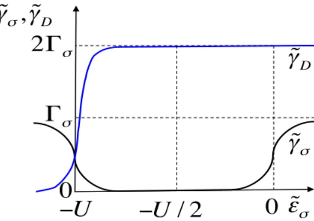
Figure 1. Schematic dependence of relaxation rates e and eD versus normalized dot level
energy " for V = B = 0 in the limit T << U .e
lower energy pole of the retarded dot electron Green function Gr(!) (i.e. " = " + Re⇧e 1(" )),e
and obtained from
e
" = " + Re⌃ 1(! =" ).e (14)
since the contribution brought by Re⌃ 4(! =" ) is negligible. In the regime whene |" µ| ,
we get e " = " X ↵ ↵¯ ⇡ log |"¯ µ↵| |"¯ + U µ↵| . (15)
The latter result is in agreement with Haldane’s result [23] obtained by using scaling theory. Besides the relaxation ratese , eD are the inverse lifetime broadening or decay rates of the
corresponding excited states with 1 and 2 electrons in the dot respectively. Those decay rates can be determined by using perturbation theory in t↵ , leading to the generalized Fermi golden
rules, the excited state playing the role of the initial state|i > in the perturbation theory. Up to the fourth order in t↵ , ,D = (2),D+
(4) ,D where (2) ,D = 2⇡ P |f>| < f|HT|i > |2 (Ei Ef) and (4) ,D = 2⇡ P
|f>|P|int> < f|HT|int > Ei 1Eint < int|HT|i > |2. (Ei Ef). HT is the tunneling
part of the hamiltonian, |i > is the initial state with energy Ei, |f > and |int > are all the
possible final and intermediate states with energies Ef and Eint respectively. The calculation
is straightforward. The only complication comes from the fact that one must systematically consider all the possible processes by which the initial state can desintegrate (all possible final and intermediate states) provided that Ei = Ef while letting the possibility to pass through
distinct intermediate states in back and forth paths respectively as taken into account by the summation over the intermediate states |int > in the analytical expression of (4),D given above. Incorporating the normalization of the dot level energy, we obtain the following results
e(2) =X ↵ h ↵ [1 nF("e µ↵)] + ↵¯nF("e¯+ U µ↵) i , (16) eD(2) = X ↵ h ↵ [1 nF(" + Ue µ↵)] i , (17) e(4) = 1 2⇡ X ↵ Z d"[1 nF(" µ ) i · h nF(" µ↵){ ↵ (" " )e 2 + ↵¯ ¯ (" "e¯ U )2} + nF (" +"e¯ "e µ↵) ↵¯ { 1 " "e¯ U 1 " "e } 2i,
(18) eD(4) = 1 2⇡ X ↵ , Z d"[1 nF(" µ )] 1 (" "e U )2 · h nF(" µ↵) ↵ + [1 nF(" +e "e¯ + U " µ↵)] ↵ ¯ i . (19)
This result constitutes a generalization of the results of [11, 24] to any value of U . Indeed in [11, 24], since only the infinite U limit is considered, eD is not accounted for and the result
for e contains the infinite U contribution only. Moreover these expressions can be seen as an extension of the results of [13] obtained by pushing the truncation of the set of EOM up to following orders. At equilibrium and in the absence of magnetic field, the 4th order contributions in t to bothe and eD are zero; e andeD at V = B = 0 are then simply given by their second
order terms, the dependence of which as a function of" are represented in Figure 1. Notice thate e at V = B = 0 is zero at the particle-hole symmetric point whereas it equals ¯ =P↵ ↵¯
and =P↵ ↵ respectively in the empty and doubly occupied dot regimes. Moreover eD at
V = B = 0 shows an abrupt increase around the doubly-occupied dot regime before saturating to ( + ¯). At finite bias or finite magnetic field, the fourth order contributions e(4) and eD(4)
becomes nonzero. The respective deviations towards the values obtained at V = B = 0 are found to be linear in either V or B.
5. Results about the spectral density and the linear/ di↵erential conductances out of equilibrium
In this section we restrict our discussion to the situation where the magnetic field is zero. The spin-dependent spectral density in the dot is obtained from the retarded Green function: A (!) = ImGr(!)/⇡. The spectral density exhibits a series of peaks identified as the poles of
the retarded Green function. We list them below:
- the lower and upper energy poles already discussed in section 4, located at" ande " + U ,e leading to the formation of the two broad peaks in the spectral density centered around these values;
- two additional poles arising at µ↵ for temperature lower than the Kondo temperature TK
resulting from the logarithmic singularities of ⌃ 1(!) and ⌃ 4(!) around these values leading
to the formation of a split Kondo resonance with two peaks pinned at the chemical potential of each lead. The splitting of the Kondo peak is equal to the bias voltage energy eV .
To be exhaustive, we will mention the presence of another pole at µ↵+" +e "e¯ + U due
to the logarithmic singularities of ⌃ 1(!) and ⌃ 4(!) at these values, brought by the second
term in the r.h.s. of the expressions given in Eq.(6) for the self-energies ⌃ i(!). This pole
leads to the formation of a spurious peak of negative intensity (antiresonance) in the spectral density. However we point out that these latter logarithmic singularities are washed out by the large value of the inverse lifetime broadening eD(4) as evaluated in section 4. As a result, this spurious peak is no longer present in our theory. This solves a long-standing unsolved problem about the existence of this spurious peak pointed out in previous works and which was all the more undesirable that it just compensates and destroys the Kondo peak at the particle-hole symmetric point and makes the Kondo e↵ect paradoxically disappear at that point. We end up by showing that the Green function in the dot at the energies µ↵ fulfills the unitary condition:
|Gr(µ
↵)|2 = ImGr(µ↵)/ . To prove this, we evaluate L (!) and M (!) in the vicinity of
µ↵. Noticing that at low temperature n! "+iF(" µ↵) varies strongly at "⇠ µ↵ whereas Ga(") varies
smoothly, one can write for ! ⇠ µ↵
L (!) = X ↵ ↵ ⇡ G a(!)hln|µ↵ !| D + i⇡nF(!) i , (20) 6
M (!) = X ↵ ↵ ⇡ [1 + i G a(!)]hln|µ↵ !| D + i⇡nF(!) i . (21)
Both of these functions show logarithmic singularities around ! = µ↵. Hence the self-energies
⌃ 1(!) and ⌃ 4(!) at T = 0 takes the following form at ! ⇠ µ↵
⌃ 1(!) = X ↵ ↵ ⇡ G a(!) ln µ↵ ! D , (22) ⌃ 4(!) = X ↵ ↵ ⇡ [1 + i G a(!)] ln µ↵ ! D . (23)
Incorporating the last two expressions into Eq.(2), we show that the dot electron Green function at ! = µ↵ writes Gr(µ↵) = Ga(µ ↵) 1 + 2i Ga(µ ↵) . (24)
The solution to this equation is of the form: Gr(µ↵) = exp i (µ↵)sin (µ↵)/ . At the value of
the chemical potential in the leads ! = µ↵, the dot electron Green function fulfills the following
relation: |Gr(µ
↵)|2= ImGr(µ↵)/ usually referred to as the unitary condition. As a result:
A (µ↵) = sin2 (µ↵)/(⇡ ). Then in the case when the dot is symmetrically coupled to the
leads ( L = R ), the S-matrix at the chemical potential µ↵ obtained from S (!) = 1 iT (!)
with T↵ (!) = 2p ↵ Gr(!) simply writes
S (!) = exp i (µ↵) ✓ cos (µ↵) isin (µ↵) isin (µ↵) cos (µ↵) ◆ . (25)
Determining the precise value of (µ↵) supposes to solve the self-consistency Eq.8 for < n >
which requires the knowledge of the Green function over the whole energy range and not only at the values of the chemical potentials. At equilibrium the phase shift at the chemical potential obeys the Friedel sum rule ↵(µ↵) = ⇡n , corresponding to the complete screening of the spin in
the dot by the spin of the conduction electrons in the leads and A (µ↵) = sin2⇡n /(⇡ ). At the
particle-hole symmetric point (µ↵) = ⇡/2 leading to the unitary limit with A (µ) = 1/(⇡ ).
In the steady state, the dc-current can be calculated by using Meir and Wingreen’s formula [25] generalizing Landauer formula to the interacting case. In the case when L (!) and R (!)
are proportional to each other, i.e. L (!) = R (!), the dc-current for spin is expressed
as a function of the retarded Green function in the dot. The linear conductance dI /dV in the limit V going to zero, is found to reach the unitary limit at the particle-hole symmetric point and the di↵erential conductance dI /dV at finite V decreases with increasing V giving rise to a zero bias peak of width TK around V = 0 followed by a broad peak at higher bias. The results
will be presented in more details in a forthcoming paper [20]. 6. Conclusion
In this paper we have generalized the equation of motion approach to the situation of a quantum dot driven out of equilibrium by the application of a dc bias voltage. The main ingredients that we have incorporated are the following: (i) We have considered all possible decoupling parameters with equal spin: hn i, hc†k0↵¯ck↵¯i and the mixed parameter hf¯†ck↵¯i
in order to truncate the set of equations of motion of the Green functions which has then been solved; (ii) We have shown that, provided that the system is its steady state, the various decoupling parameters can be obtained self-consistently from the knowledge of the retarded Green functions only, even if the fluctuation-dissipation theorem does not hold any longer; (iii) We have systematically considered the normalization of the bare dot level energy introduced by
the self-energy corrections corresponding to the dressing of the bare propagators, and (iv) We have taken into account the normalized inverse lifetime broadening of the various excited states by using the Fermi golden rules. We have thus derived the retarded electronic Green function in the dot and deduced the spectral density. The spectral density exhibits two broad peaks centered around the normalized dot level energies. The Kondo resonance formed at low temperature is split by the bias voltage with the two peaks pinned at the chemical potentials of each of the two leads. The merit of the approach developed is to enable us both to recover the unitary condition for the density of states at the split resonance peak and to cure the long-standing problem about the presence of spurious peak in the density of states. In this way the quantum dot driven out of equilibrium feels a strong Kondo e↵ect at the particle-hole symmetric point. Finally we have discussed the evolution of the linear and the di↵erential conductances as a function of gate and bias voltages when the quantum dot is driven in its steady state.
Acknowledgments
We wish to thank Shiue-yuan Shiau and Rapha¨el Van Roermund for helpful discussions at the early stage of the work, Adeline Cr´epieux, Harold Baranger, Soumya Bera and Shaon Sahoo for stimulating discussions. The work has been funded by the Indo-French Centre for the Promotion of Advanced Research (IFCPAR) under Contract No.4704 and the Nanosciences Foundation of Grenoble under RTRA Contract CORTRANO.
* Also at the Centre National de la Recherche Scientifique (CNRS) References
[1] Hewson A P 1993 The Kondo Problem to Heavy Fermions (Cambridge University Press) and references within [2] Ng T K and Lee P A 1988 Phys. Rev. Lett 47 452
[3] Glazman L and Raikh M 1988 JETP Lett. 11 2389
[4] Goldhaber-Gordon D, Shtrikman H, Mahalu D, Abusch-Magder D, Meirav U, and Kastner M 1998 Nature 391 156
[5] Cronenwett S M, Oosterkamp, and Kouwenhoven L P 1998 Science 281 165115
[6] van der Wiel W, De Franceschi S, Fujisawa T, Elzerman J, Tarucha S, and Kouwenhoven L P 2000 Science 289 2105
[7] Appelbaum J A, and Penn D R 1969 Phys. Rev. 188 874 [8] Theumann A 1969 Phys. Rev. 178 978
[9] Lacroix C 1981 J. Phys. F: Met.Phys. 11 2389; Lacroix C 1981 J. Appl. Phys. 53 2131 [10] Meir Y, Wingreen N S, and Lee P A 1991 Phys. Rev. Lett. 66 3048
[11] Meir Y, Wingreen N S, and Lee P A 1993 Phys. Rev. Lett. 70 260
[12] Kashcheyevs V, Aharony A, and Entin-Wohlman O 2006 Phys. Rev. B 73 125338 [13] Van Roermund R, Shiau S Y, and Lavagna M 2010 Phys. Rev. B 81 165115 [14] Krawiec M and Wysokinski K I 2002 Phys. Rev. B 66 165408
[15] Martinek J, Utsumi Y, Imamura H, Barna´s J, Maekawa S, K¨onig J, and Sch¨on G 2003 Phys. Rev. Lett. 91 127203
[16] Monreal R C and Flores F 2005 Phys. Rev. B 72 195105
[17] Entin-Wohlman O, Aharony A, and Meir Y 2005 Phys. Rev. B 71 035333 [18] Qi Y, Zhu J X, and Ting C S 2009 Phys. Rev. B 79 205110
[19] Balseiro C A, Usaj G, and S´anchez M J 2010 J. Phys.: Condens. Matter 22 425602 [20] Lavagna M to be published
[21] Anderson P W 1961 Phys. Rev. 124 41
[22] Ng T K 1996 J. Phys. F textitPhys. Rev. Lett. 76 487 [23] Haldane F D M 1978 Phys. Rev. Lett 40 416
[24] Wingreen N S, Meir Y 1994 Phys. Rev. B 49 11040 [25] Meir Y, Wingreen N S 1992 Phys. Rev. Lett 68 2512