HAL Id: hal-02063396
https://hal.inria.fr/hal-02063396
Submitted on 11 Mar 2019
HAL is a multi-disciplinary open access
archive for the deposit and dissemination of
sci-entific research documents, whether they are
pub-lished or not. The documents may come from
teaching and research institutions in France or
abroad, or from public or private research centers.
L’archive ouverte pluridisciplinaire HAL, est
destinée au dépôt et à la diffusion de documents
scientifiques de niveau recherche, publiés ou non,
émanant des établissements d’enseignement et de
recherche français ou étrangers, des laboratoires
publics ou privés.
Estimation of Axonal Conduction Speed and the Inter
Hemispheric Transfer Time using Connectivity Informed
Maximum Entropy on the Mean
Samuel Deslauriers-Gauthier, Rachid Deriche
To cite this version:
Samuel Deslauriers-Gauthier, Rachid Deriche. Estimation of Axonal Conduction Speed and the Inter
Hemispheric Transfer Time using Connectivity Informed Maximum Entropy on the Mean. SPIE
Medical Imaging 2019, Feb 2019, San Diego, United States. �hal-02063396�
Estimation of Axonal Conduction Speed and the Inter
Hemispheric Transfer Time using Connectivity Informed
Maximum Entropy on the Mean
Samuel Deslauriers-Gauthier and Rachid Deriche
Inria Sophia Antipolis M´
editerran´
ee, Universit´
e Cˆ
ote d’Azur, France
ABSTRACT
The different lengths and conduction velocities of axons connecting cortical regions of the brain yield information transmission delays which are believed to be fundamental to brain dynamics. A critical step in the estimation of axon conduction speed in vivo is the estimation of the inter hemispheric transfer time (IHTT). The IHTT is estimated using electroencephalography (EEG) by measuring the latency between the peaks of specific electrodes or by computing the lag to maximum correlation on contra lateral electrodes. These approaches do not take the subject’s anatomy into account and, due to the limited number of electrodes used, only partially leverage the information provided by EEG.
Using the previous published Connectivity Informed Maximum Entropy on the Mean (CIMEM) method, we propose a new approach to estimate the IHTT. In CIMEM, a Bayesian network is built using the structural connectivity information between cortical regions. EEG signals are then used as evidence into this network to compute the posterior probability of a connection being active at a particular time. Here, we propose a new quantity which measures how much of the EEG signals are supported by connections, which is maximized when the correct conduction delays are used.
Using simulations, we show that CIMEM provides a more accurate estimation of the IHTT compared to the peak latency and lag to maximum correlation methods.
Keywords: Inter hemispheric transfer time, axon conduction velocity, diffusion MRI, EEG, MEG
1. INTRODUCTION
The different lengths and conduction velocities of axons connecting cortical regions of the brain yield information transmission delays which are believed to be fundamental to brain dynamics.1,2 While early work on axon conduction velocity was based on ex vivo measurements,3,4 more recent work makes use of a combination of diffusion Magnetic Resonance Imaging (MRI) tractography and electroencephalography (EEG) to estimate axon conduction velocity in vivo.5,6 An essential intermediary step in this later strategy is to estimate the inter hemispheric transfer time (IHTT) using EEG. The IHTT is estimated by measuring the latency between the peaks of specific electrodes or by computing the lag to maximum correlation on contra lateral electrodes.7 These approaches do not take the subject’s anatomy into account and, due to the limited number of electrodes used, only partially leverage the information provided by EEG.
In previous work,8,9 we proposed a method, named Connectivity Informed Maximum Entropy on the Mean (CIMEM), to estimate information flow in the white matter of the brain. CIMEM is built around a Bayesian network which represents the cortical regions of the brain and their connections, observed using diffusion MRI tractography. This Bayesian network is used to constrain the EEG inverse problem and estimate which white matter connections are used to transfer information between cortical regions. In our previous work, CIMEM was used to infer the information flow in the white matter by assuming a constant conduction velocity for all connections. In this context, the conduction speed, and thus the delays, were inputs used to help constrain the
Further author information: (Send correspondence to S.D.G.)
S.D.G.: E-mail: [email protected], Telephone: + 33 4 92 38 75 91 R.D.: E-mail: [email protected], Telephone: + 33 4 92 38 78 32
problem. Here, we interchange the variables and the parameters and instead assume that the connection used to transfer information across the hemispheres is known, due the design of the acquisition paradigm, but that its conduction velocity must be estimated. The result in a novel method to estimate the IHTT in addition to the axon conduction velocity that makes full use of the information provided by EEG and diffusion MRI.
2. METHODS
Our strategy to estimate the IHTT is built on a generative model of the EEG measurements which incorporates both the cortical surface and the underlying white matter connections. To make the current document self contained, we briefly summarize this generative model here. A more detailed presentation and discussion is available in our previous work.8,9
2.1 CIMEM Generative Model and Inverse Problem
The sources of brain activity are distributed on the cortical surface with their orientations fixed and normal to the surface. Let x = [x1,1, x2,1, ..., xN,1, x1,1, ...xN,T] ∈ RN T be the concatenated vector of source intensity where
N is the number of sources and T is the number of time samples. These sources of brain activity are related to the EEG measurements through the forward model10
m = Gx (1)
where m ∈ RM T
is the concatenation of M measurements at each time sample. The matrix G ∈ RM T ×N T
is the lead field matrix which projects sources onto sensors and is a known quantity. Because our formulation considers all time samples simultaneously, the lead field matrix is block diagonal with each block containing the usual lead field matrix.
In theory, any vector of source activity x can be used in the forward problem of Equation1to generate the measurements m. In practice however, certain configuration are more likely than others. For example, x can be expected to contain spatial correlation between neighboring sources and temporal correlation between sources connected by white matter axons. To capture the spatial correlation, we parcellate the brain into NS regions,
assign a state Sk to each, and group them in a region state vector S. The state of a cortical region provides
information about the intensity of the individual sources within the region. For example, it can be expected that the sources of a region that is in the active state will have a higher average intensity than the sources in a region that is in an inactive state. To capture the temporal correlation, we connect the brain regions using NC white
matter connections, assign a state Ci to each of them, and group them in a connection state vector C. It is
essential to note that, at the temporal resolution of EEG, white matter connections do not transfer information instantaneously. The callosal axons of the splenium, for example, are between 150 to 200 mm long and introduce a communication delay of 25 to 35 milliseconds between the left and right occipital lobes, assuming a conduction velocity of 6 m/s.3 These delays are well above the millisecond temporal resolution of EEG. Connections in our model therefore introduce activation delays that reflect the length and conduction velocity of axons. As such, the state of a connection provides information on the cortical regions it connects across time and enforce a temporal regularization into the model. For example, if a connection is in the active state, it forces the regions it connects to also be in the active state with a specified delay. Here, both brain regions and connections are assigned two possible states: active or inactive. To link these states of cortical regions and connections to source intensity, we define a reference law dµ(x) = µ(x)dx which encodes our global prior knowledge of cortical source activity. Specifically, we define dµ(x) to have the form
dµ(x) =X {C} NC Y i=1 ϕ(Ci) X {S} NS Y k=1 π(Sk|Cγ(k))dµ(xk|Sk) (2)
where the sum over state vectors indicates a sum over every possible state combinations, where xk contains
the sources of the kth brain region, and where C
γ(k) is the set of connections reaching the kth brain region.
The density dµ(xk|Sk) encodes the likelihood of a configuration xk given the kth region’s state, the density
ith connection’s state. A more detailed derivation of Equation 2 is available in our prior work.9 In summary, Equation 2 reflects that the activity of sources depends on the state of the region to which they belong and that the activity of a region depends on the activity on the regions to which it is connected. Because of the hierarchical relationship between sources, regions, and connections, Equation2defines a Bayesian network which can be used to compute the likelihood of any source configuration. In addition, the Bayesian network can also be used to infer the most likely brain configuration (source intensity, region states, connection states) given the observations. This can be achieved by finding the probability law p(x) whose average fits the measurements and that is closest to the reference law dµ(x). We therefore propose to solve the problem
minimize p(x),λ,λ0 Z p(x) lnp(x) µ(x)dx − λ(m − G Z xp(x)dx) − λ0(1 − Z dp(x)) (3) where the first term is the Kullback-Leibler divergence between p(x) and µ(x), the second term is the data fit, and the third term is a scaling to ensure p(x) is a probability distribution. This can be shown11,12 to be equivalent to solving the problem
λ∗= arg min
λ
ln Z
exp (λTGx)dµ(x) − λTm (4) where λ∗completely determines the optimal p(x), λ, and λ0of Equation3. Because λ∗captures the compromise
between the EEG observation and the priors of the model, it can be used to compute a posterior probability for all variables of the model. Here, we are specifically interested in the posterior probability of active connections, defined as
Z(Ci,n= 1) =
Z
exp (λ∗TGx)dµ(x|Ci,n= 1) (5)
which is derived from the first term of Equation4.
2.2 IHTT Estimation
The original purpose of CIMEM was to map information flow in the white matter from combined EEG and diffusion MRI measurements. In this context, the conduction velocity of white matter axons must be given as an input and serves to constrain the solution space. Our suggestion was to use diffusion MRI to select the available white matter connections and attempt to identify which of them are active at a given time. The output of our algorithm was then a subset of white matter connections whose delays and cortical endpoints explain the measurements. In contrast to this approach, here we assume that the white matter connections that support the data are known, but that their conduction velocity and induced delay must be estimated. A prime example is the estimation of the IHTT, where the communication between the left and the right hemisphere is assumed to go through callosal white matter axons. An approximation of the geometry of these axons can be obtained using diffusion MRI and added to the CIMEM model while ignoring all other brain connections. For each connection of the model and at every time instant, a variable is added to the model with two possible state: active (0) or inactive (1). EEG signals are then used as evidence into this network to compute the posterior probability of a connection being active at a particular time. Recall that Z(Ci,n = 1) is the posterior probability that the ith
connection is active at the nth time point obtained by solving the CIMEM problem of Equation 4. We define
the connectivity power of the ithconnection as
Γd(Ci= 1) = N−1 N −1
X
n=0
Z(Ci,n= 1)2 (6)
for a given delay d. The connectivity power is then computed for a series of delays and the estimated delay for a given connection is the one that maximizes Γd(Ci). The rationale is that the CIMEM model will only be able
to use the connection to explain the EEG measurements if the selected delay is correct.
For comparison purposes, the IHTT was also estimated using the peak latency and lag to maximum correlation methods.7 For the peak latency method, the IHTT is estimated by computing the temporal difference between the location of the maximum magnitude on the left and right lateral occipital electrodes. For the correlation method, the Pearson correlation is computed between the left and right lateral occipital electrodes for all time lags and the lag with maximal correlation is selected.
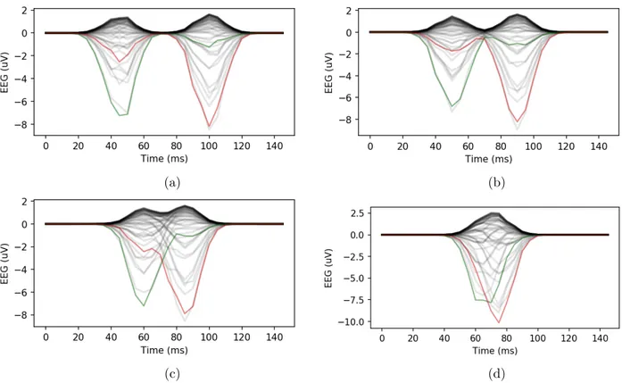
(a) (b)
(c) (d)
Figure 1. Examples of simulated EEG signals for a delay of 11, 8, 5, and 2 samples (a, b, c, d). The left and right lateral occipital sensors are displayed in green and red, respectively. All the other sensors are displayed in grey.
2.3 Data Simulation
To evaluate the performance of our algorithm, EEG signals were generated using a realistic head geometry and acquisition montage with 63 electrodes. The cortical surface used for simulation was reconstructed from a T1 weighted MRI of a healthy subject using FreeSurfer and decimated to 8000 vertices. EEG signals were generated by selecting the sources of the left and right lateral occipital cortical regions and assigning them intensities using a multivariate Gaussian with a mean of 1 and a covariance based on the cortical distance between sources. The left and right sources were then modulated by two temporal Gaussians with a variance of 80 ms whose difference in mean was adjusted to obtain the desired delay. The forward operator used to project cortical activity onto sensors was computed using OpenMEEG13with the source locations corresponding to the vertices of the cortical surface.
3. RESULTS
Examples of the simulated EEG signals are illustrated in Figure 1. As the delay between the left and right activation is reduced, both waveforms merge to produce a single peak. In addition, due to volume conduction, the peak does not occur at the same location on all electrodes. This effect will be more pronounced as the width of the activation, i.e. its duration, is increased. As both the peak latency and correlation methods rely only on the shape of the recorded signal, this will have an effect on their estimation of the IHTT.
A few representative examples of the connection power computed using CIMEM as a function of the simulated delay are illustrated in Figure2. The EEG measurements were simulated with a delay of 11, 8, 5, and 2, which corresponds to a conduction speed of 1.82, 2.5, 4, and 10 m/s, respectively, for a white matter connection of 100 mm and EEG signals sampled at 200 Hz. In all cases, we observe that the maximum of the connection power curve corresponds to the simulated delay illustrated by a vertical red line in the graphs.
(a) (b)
(c) (d)
Figure 2. The connection power (Γ) as a function of the delay used for the reconstruction for simulated delays of 11, 8, 5, 2 samples (a, b, c, d). The maximum connection power corresponds to the simulated delay illustrated by the red vertical line.
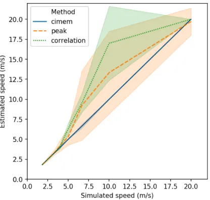
The mean estimated speed as a function of the simulated speed is illustrated in Figure 3. Both the peak and correlation method overestimate the conduction speed for simulated speed of 5 to 10 m/s. For the Gaussian waveform simulated in this study, these speeds correspond to the range where the left and right occipital activa-tions overlap. As previously illustrated in1, this distorts the shape of the waveform observed on the electrodes and shifts the position of the peak. On the other hand, the mean speed estimated with CIMEM more closely corresponds to the true simulated speed as the volume conduction, the anatomy of the subject, and all electrodes are taken into account.
4. CONCLUSION
The estimation of the inter hemispheric transfer time is a critical step in the estimation of in vivo axon conduction velocity. Current methods rely on sensor space delays and thus do take the subject’s anatomy into account. In this work we have presented a new method to estimate the inter hemispheric transfer time and thus axon conduction velocity. Our new approach, based on our previously published CIMEM algorithm, takes the subjects anatomy into account and leverages all of the information provided by EEG. In simulations, CIMEM outperforms both the peak latency and lag to maximum correlation methods for the estimation of the IHTT.
A hypothesis that is common to the peak latency, lag to maximum correlation, and our method is that the inter hemispheric transfer time can be represented by a single value. In practice, due to the distribution of axonal diameters in the white matter,14 using a distribution of values may be more realistic. We believe our method may be adapted to provide this information and modifying it is the topic of our current work.
In addition to estimating white matter delays and thus providing an insight into brain dynamics, our method may also be used to probe the microstructural information of specific white matter bundles. For example, it has been shown that axon diameters and myelin both affect axon conduction velocity.3,15 Therefore, by providing an estimate of conduction velocity, our could potentially be used to validate in vivo microstructure estimates provided by diffusion MRI.
Figure 3. Mean estimated speed as a function of the simulated speed in meters per second for the peak, correlation, and CIMEM approaches. The speed is computed from the IHTT for a connection with a length of 100 mm and EEG signals sampled at 200 Hz. The shaded area indicates the standard deviation for each method.
ACKNOWLEDGEMENTS
This work has received funding from the European Research Council (ERC) under the European Union’s Horizon 2020 research and innovation program (ERC Advanced Grant agreement No 694665 : CoBCoM - Computational Brain Connectivity Mapping).
REFERENCES
[1] Deco, G., Jirsa, V., McIntosh, A. R., Sporns, O., and Kotter, R., “Key role of coupling, delay, and noise in resting brain fluctuations,” Proc Natl Acad Sci 106(25), 10302–10307 (2009).
[2] Caminiti, R., Carducci, F., Piervincenzi, C., Battaglia-Mayer, A., Confalone, G., Visco-Comandini, F., Pan-tano, P., and M., I. G., “Diameter, length, speed, and conduction delay of callosal axons in macaque monkeys and humans: Comparing data from histology and magnetic resonance imaging diffusion tractography,” The Journal of Neuroscience 33(36), 14501–14511 (2013).
[3] Hursh, J. B., “Conduction velocity and diameter of nerve fibers,” American Journal of Physiology 127(1), 131–139 (1939).
[4] Ritchie, J. M., “On the relation between fibre diameter and conduction velocity in myelinated nerve fibers,” Proc. R. Soc. Lond. 217, 29–35 (1982).
[5] Horowitz, A., Barazany, D., Tavor, I., Bernstein, M., Yovel, G., and Assaf, Y., “In vivo correlation between axon diameter and conduction velocity in the human brain,” Brain Struct Funct 220, 1777–1788 (2015). [6] Innocenti, G. M., Caminiti, R., and Aboitiz, F., “Comments on the paper by horowitz et al. (2014),” Brain
Structure and Function 220(3), 1789–1790 (2015).
[7] Saron, C. D. and Davidson, R. J., “Visual evoked potential measures of interhemispheric transfer time in humans,” Behavioral Neuroscience 103(5), 1115–11138 (1989).
[8] Deslauriers-Gauthier, S., Lina, J. M., Butler, R., Bernier, P. M., Whittingstall, K., Deriche, R., and De-scoteaux, M., “Inference and Visualization of Information Flow in the Visual Pathway using dMRI and EEG,” in [MICCAI 2017 Medical Image Computing and Computer Assisted Intervention ], (2017).
[9] Deslauriers-Gauthier, S., Lina, J. M., Butler, R., Bernier, P. M., Whittingstall, K., Deriche, R., and De-scoteaux, M., “White Matter Information Flow Mapping from Diffusion MRI and EEG,” NeuroImage, in review .
[10] Baillet, S., Mosher, J. C., and Leahy, R. M., “Electromagnetic brain mapping,” IEEE Signal Processing Magazine 18(6), 14–30 (2001).
[11] Jaynes, E. T., “Information theory and statistical mechanics,” Physical Review 106(4), 620–630 (1957). [12] Amblard, C., Lapalme, E., and Lina, J. M., “Biomagnetic source detection by maximum entropy and
graphical models,” IEEE transactions on bio-medical engineering 51(3), 427–42 (2004).
[13] Gramfort, A., Papadopoulo, T., Olivi, E., and Clerc, M., “OpenMEEG: opensource software for quasistatic bioelectromagnetics,” Biomedical engineering online 9, 45 (2010).
[14] Liewald, D., Miller, R., Logothetis, N., Wagner, H. J., and Schuz, A., “Distribution of axon diameters in cortical white matter: an electron-microscopic study on three human brains and a macaque,” Biological Cybernetics 108, 541–557 (2014).
[15] Drakesmith, M. and Jones, D. K., “Mapping axon conduction delays in vivo from microstructural MRI,” bioRxiv (2018).