Astronaut adaptive arm motions on the MIR Space Station : kinematic analysis

Astronaut Adaptive Arm Motions

on the MIR Space Station:

Kinematic Analysis

by

Karen Thibault

Submitted to the Department of Physics in partial fulfillment of the requirements for the degree

Bachelor of Science

at the

MASSACHUSETTS INSTITUTE OF TECHNOLOGY

©Massachusetts Institute of Technology 1998. All rights reserved.

Author... ... Department of Physics May 15, 1998 Certified... ... Dava J. Newman Associate Professor Thesis Advisor Certified... ... ... Claude R. Canizares Physics Professor A ccepted ... June L. Matthews

Astronaut Adaptive Arm Motions on the MIR

Space Station: Kinematic Analysis

by Karen Thibault

Submitted to the Department of Physics on May 15, 1998, in partial fulfillment of the requirements of the degree of

Bachelor of Science

Astronauts exposed to the microgravity conditions of space flight often have difficulty executing simple tasks that require neuromuscular motor control, such as closing their eyes and pointing to an object, during their initial adaptation to reduced gravity. This leads astronauts to adjust some of their motions while in space. Gaining an understanding of astronauts' adaptation is an essential step to constantly improve the design of future space missions from a human factors perspective. The aim of the present study is to investigate the ways that astronauts adapt arm throwing motions over the course of long duration space flight. Specifically, it focuses on the kinematics of adaptive arm motions for subjects attempting to toss a ball at a target.

The experiment originated as part of a study using the Man-Vehicle Lab's Enhanced Dynamic Load Sensors (EDLS) to measure the magnitude and frequency of disturbances to the microgravity environment caused by astronauts on the Russian space station Mir. The results are used to characterize astronaut-induced loads during space flight. Such information is critical in defining engineering design requirements for the International Space Station (ISS) and ensuring future mission success. EDLS sessions included passive and active use of the sensors. Throwing tasks were one example of active data collection. This type of data is important for determining the impact of routine activities on the microgravity environment of the ISS.

In this study, data is examined from throws executed by one astronaut during two sessions. Throws were made with both hands and with eyes open and closed. The results show that the astronaut altered his throwing style in space significantly from his normal 1-g earth throw. However, only minor adaptations occurred between successive sessions since the subject in this experiment was previously well adapted to the microgravity environment of space. The movement of the shoulder, elbow and wrist are examined. Adaptations include changes in acceleration patterns, release speed, and windup length. In addition, significant variations are witnessed between throws that subject made with their eyes open and closed. Throws made with eyes open were more consistent and symmetrical with respect to flexion and extension phases. More work must be done before results are conclusive, but it appears that throws become smoother and more direct over time. Also, astronauts overcome remaining perceptive and proprioceptive difficulties when they have visual feedback.

Thesis Advisor: Dava J. Newman

Table of Contents

List of Figures

Figure 3.1. Astronaut Subject Body Model... 9

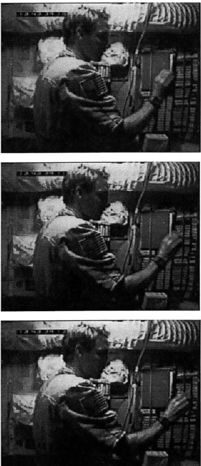
Figure 3.2. Three Consecutive Frames of a Throw ... 10

Figure 4.1. Stick-Arm M odel... .13

Figure 4.2. W rist Trajectory ... .14

Figure 4.3. W rist Trajectory ... .16

Figure 4.4. Average W rist Velocity ... 17

Figure 4.5. W rist Velocity... .18

Figure 4.6. Elbow Angle ... .21

List of Tables

Table 4.1. Maximum Wrist Extension Velocity... 18

Table 4.2. Minimum Wrist Extension Velocity... 19

Table 4.3. Elbow Angle ... .20

Table 4.4. Shoulder Translation ... 22

1.

Introduction

Astronauts experience a variety of physiological changes when they encounter the microgravity environment of space flight. Some examples of physiological adaptation include altered vestibular system responses, atrophy of muscles, and decalcification of the skeletal tissue. While these conditions are not life threatening on short duration space flights (<30 days), they can cause reason for concern about astronaut health. Vestibular disorientation can cause motion sickness and interfere with the execution of manual tasks, but only lasts for a few days. Long term space flight can cause deterioration of muscle

(20-30% atrophy) or bone (1% density loss per month) tissue that could make an emergency egress impossible for an astronaut upon returning to the normal gravity of Earth. For these reasons, understanding the causes and effects of altered human physiology is a critical step for successful long-term space (months to years) habitation.

Many other reactions to microgravity are observed by astronauts. These include dizziness, loss of motor-sensory coordination, and difficulties with proprioception or the knowledge of how the limbs are positioned relative to the body (N.A.S., 1998). These reactions are generally encountered soon after entering microgravity and tend to disappear quickly (Gerathewohl, 1957 ). In addition astronauts have reported difficulties with hand-eye coordination that occur during long flights, and problems with depth perception were reported on the Russian space station Mir (N.A.S., 1998).

As a result of these altered responses, astronauts exposed to microgravity conditions during space flight often have difficulty executing simple tasks that require neuromuscular motor control. Subjects exposed to microgravity cannot accurately point to an object with closed eyes. They may, however, adapt to microgravity and improve their performance over time. Visual feedback plays a critical role in this adaptation (Bock, et al.,

This study investigates the effects of prolonged exposure to microgravity on an astronaut's ability to throw a ball at a target. It focuses on the ways that astronauts adapt their throwing motions in space and explores which types of adapted motions are optimally suited to improving accuracy. In addition, the role of visual feedback is examined.

This study is part of a series of experiments using Enhanced Dynamic Load Sensors (EDLS). The EDLS system uses sensors to record the magnitude and frequency of disturbances to the microgravity environment caused by astronauts on the Russian space station Mir. The throws were conducted by subjects whose feet were confined in EDLS foot restraints as part of the active data collection sessions. Data recorded, in this way, can be used to characterize astronaut-induced loads during space flight. This information is critical in defining engineering design requirements for the ISS and for determining the impact of routine activities on its microgravity environment.

2.

Background

Aerospace medicine has long been concerned with the effects of altered gravity on humans. In the past, studies have shown that transition from 1-g to a microgravity environment results in performance degradation (Young, et al., 1986, Whiteside, 1961, Gerathewohl, et. al., 1957). Further, studies have shown that these phenomena are linked to perceptual difficulties (N.A.S., 1998). Subjects exposed to microgravity may suffer from proprioceptive illusions (Cohen, 1970). In addition, problems with depth perception

were reported on Mir (N.A.S., 1998). However, subjects could often compensate for impaired hand-eye coordination if they had visual feedback (Cohen, Welch, 1988). In one

study, subjects who initially had trouble pointing to a target improved over time. Visual

feedback was shown to be an important tool in the adaptation process (Bock et al., 1992).

Subjects without visual feedback did not improve their aim.

subjects in water up to their necks. While these experiments did indicate that adaptation

occurred during exposure to altered gravity, they were not of adequate duration to fully

explore the extent of this adaptation (Bock, et al., 1992, Cohen, et al., 1970).

In addition to perceptual difficulties, exposure to microgravity affects manipulation

and locomotion. Posture, locomotion, and balance parameters change in microgravity. As

a result, muscles are loaded and used differently (N.A.S., 1998). The current experiment

researches the effects of long term space flight on neuromuscular motor control. While,

past studies investigated the ability of humans to perform certain tasks before and after

exposure to altered gravity (Newman, et al., 1997), this experiment investigates the ways

astronauts adjust to changes in their perception and motor control during prolonged

exposure to a reduced gravity environment.

The subjects in this experiment executed arm throwing motions while held down by

foot restraints. The restraints were attached to Enhanced Dynamic Load Sensors which

recorded the forces and torques exerted by the subjects. The purpose of the EDLS

experiment is to asses the magnitude and frequency of astronaut-induced disturbances to

their microgravity environment. This information is necessary to accurately define

engineering design requirements for the International Space Station (ISS) and ensure future

mission success. One of the key missions of the ISS is to perform microgravity science

experiments that require ~10A4 to OA7g's. Astronaut movements on board the ISS could

disturb this state. The EDLS experiment is designed to assess the impact that astronauts

have on the microgravity environment.

EDLS sessions included passive and active use of the sensors. Throwing tasks

were one example of active data collection. Since astronauts adapt their neuromuscular

motor control as they become used to microgravity (Cohen, 1970), the impacts of their

routine actions may also change. For this reason, it is important to study how adaptation to

The aim of the present study is to quantify the ways that astronauts adapt motions

over the course of extended-duration space flight. Specifically, it focuses on a kinematic

analysis of the ways that astronauts adapt arm throwing motions to be more effective in

space. The subjects who participated were onboard the Russian space station Mir for

several months. By analyzing the kinetics of arm motions during their throws, it is

possible to see how astronauts, while becoming acclimated to their microgravity

environment, perform novel, goal-orientated tasks. This allows an examination of how

their throwing strategies evolve as they become more used to microgravity. Understanding

these changes may enable future scientists to recognize a general pattern of adaptation to

reduced gravity, and make more informed assessments of human performance across the

entire spectrum from g-g to 1 -g.

3.

Methods

From March to September, 1996 and January to June, 1997, seven astronauts and

cosmonauts performed the EDLS experiment, including the active operations, on the

Russian Space station Mir. In the experiment, subjects threw a ball about 1.5 cm in

diameter (made out of duct-tape) at a target. The target was placed approximately 1.5 m in

front of the subject, and was rectangular ( 25 cm x 30 cm) in shape with a bull's eye marked in the center. The subjects aimed for the bull's eye. Hash marks divided the axes

into 1 cm segments, and accuracy in the x and y directions was recorded. The throws were

videotaped by a camera that was placed perpendicular to the subject, and hence to the

direction of the throw as shown in Figure 3.1. to measure arm kinematics during the

2

camera

Figure 3.1. Camera position

The subject's head and torso appear in the video, and three small tape markers were placed

on the subjects joints as shown in Figure 3.1. Figure 3.2. is a series of 3 consecutive

Each subject who performed a session of throws did them in a specific order. First, the ball was thrown five times with eyes closed, and then, five times with the eyes open using the right arm. Next, the subject threw five times with eyes closed and five times with eyes open using his or her left arm. The subjects threw right-handed and immediately turned 180 degrees to throw left handed. The target was also moved to the opposite end of the module. This allowed the subjects to execute all 20 throws in

succession without having to move the camera. For the throws classified as "eyes closed", the subject looked at the target, closed his eyes, threw the ball, and opened his eyes to see how accurate the throw was.

In addition to making the throws, each subject would hold the target up for the video camera at their position at the start of each session for calibration purposes. The measurements for each throw include video of the arm, information on the error of each throw in the x and y directions, and data from the EDLS sensors that measure forces and torques exerted by the astronauts feet which were restrained during the throws.

3.1. Data Analysis

Upon return of the video tapes from Mir, a digital VCR was used in conjunction with Adobe Premiere software to convert the video into a series of digitized images of the individual frames. These images were further converted to a jpeg format for analysis. Next, a the Matlab program (see Appendix A) was used to obtain kinematic information on arm position and joint angles. This was done by cycling through each frame of a throw and manually registering the joint marker positions. Calibration was done at this point by using the known distances recorded on the video of the subject holding up the target. The

result of this process was a file corresponding to each throw containing 2 dimensional position data for the subject's joints in every frame. This manual digitization process was

very time intensive and the data from all seven subjects results in approximately 24,000 images.

Next, additional Matlab routines were used to analyze arm position in each frame. These programs are included in Appendix B. The first routine produces graphs of wrist

positions and velocities during throws. The second set of routines computes the angle of the elbow joint during throws. Additional information such as shoulder translation was

also extracted from the data files about each throw.

3.2. Dynamic Analysis of Throwing Motion

This analysis allows a comparison of the way astronauts throw when they enter

space to the changes that occur when they adapt to reduced gravity. A dynamic analysis of

throwing motions shows that if astronauts threw balls in space as they do on Earth they

would wildly miss the target. As a result, the fact that they hit the target is an indication of

some adaptation. The analysis described above is designed to discover the ways that they

alter their throwing technique as they repeat the task on subsequent days of their mission.

Another facet of the analysis results form the fact that each astronaut made some

throws with eyes open and some with eyes closed. The comparison of these throws can

now be used to assess the visual sensory input to the motor control system. This

information should contribute to the overall understanding of how people move in space

which will help in the design of future missions.

Do to time constraints, only the throws made by the U.S. astronaut on March 6,

1997 and March 26,1997 will be examined in this thesis. He arrived on the station on

January 12, 1997; thus, he had been exposed to microgravity conditions for 53 days and

4.

Results

The results of this kinematic analysis can be divided into three categories, namely,

data about the wrist, the elbow, and the shoulder. The data from one of the throws has

been used to construct the stick-figure diagram in Figure 4.1. It shows the arm position

during every other frame of a 2 second throw. The subject began the throw with the arm

held out (marked with a circle), bent it inward, and then extended it away from his body.

The end of the throw is marked with an "x". The stick diagram demonstrates several

features of the throw: the symmetry of the wrist movement during the flexion and extension

phases of the throw, the small shoulder translation, and the elbow movement. The elbow

was both bent and brought closer to the torso during flexion. Elbow translation suggests

that a small amount of shoulder rotation occurred as well. The axes in the diagram are

divided into 5 centimeter segments.

4.1.

Wrist Motion

Various types of results are shown for wrist motion, including comparing the wrist

trajectories during throws, examining the x and y components of this motion, and plotting

the wrist velocities. After highlighting the features of each type of data, it is possible to

compare specific throws and look for trends over time.

The motion of a subject's wrist during a throw is, of course, very similar to the

trajectory traced out by the hand. The path that the subject's wrist follows includes a

preparatory pause before the start of the motion, a windup period, the forward motion, and

the release of the ball. These features are all present in the graph of wrist trajectory in

Figure 4.2. The throw started at the clump of points in the center, moved to the left, and

then to the right.

JL2 RCO.mat -31 - -32--33 -34 --35. -36-I II I I 58 59 60 61 62 63 64 x (cm)

The trajectory traced by the wrist is broken down in its x and y components for two throws in Figure 4.3. The left hand side of the figure presents data for a throw executed while the subject had his eyes closed and the right side while he had them open. The subject used his right hand for both throws. The figure is representative of most throws and demonstrates the main difference between throws made with eyes open and closed.

In all throws, the x component of the motion is much larger than the component of the motion in the y direction. Another feature of most throws is that extension portion of the throw is at the same height as the flexion portion . In a few throws the extension

portion of the throw is slightly higher and more level. The primary difference between throws made with eyes closed and open is the relative length of the flexion and extension phases. Throws that subjects made with closed eyes generally have flexion phases which are significantly shorter than their extensions. However, extensions are still similar in length to those of throws made with open eyes. Graphs of the trajectories of all of the throws are included in Appendix C. Upon examining the graphs from groups of throws, it becomes apparent that the trajectories became steeper over time. This is also shown in the graphs of x and y position that follow the trajectory graphs in Appendix C..

JL2-RC-04 JL2-RO-04

20

20

15

15

5

.5

0o

01

0

5

10

15

0

5

10

15

15

15

5

5

0

6

0

0

50

0

50

.is

5

0

0

0

50

0

50

4.3. Comparison of a throw during session 1 with eyes closed to one with eyes open. Graphs show wrist trajectory, and displacement in the x and y directions respectively.

In Figure 4.2. each point represents the wrist position during one frame of the

video of the throw. Thus, it is possible to see that the velocity is the greatest during the

forward throwing motion just before the ball is released. The velocity curves for a right

2 1.8-1.6 E j 1.4-1.2 - U-U, o 0.8 ) c' 0.6 C) 0.4-0.2 0 0.2 0.4 0.6 0.8 1 1.2 1.4 1.6 1.8 2 Time (s)

Fig.4.4. Average wrist velocity.

The velocity curves for the throws have three main features. They start out flat at a

value near zero during the subjects preparatory pause, they have a small smooth rise and

fall during the flexion phase of the throw, and they have a large steep peak representing the arm extension. Both peaks are largely symmetrical and the extension peak velocities are 2

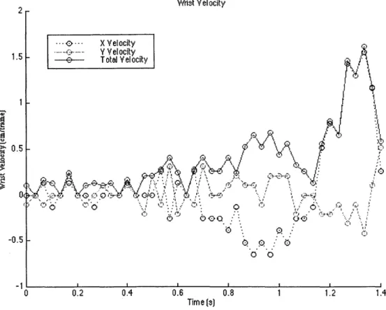
to 3 times larger then the peak flexion velocities. Figure 4.5. has been included to show the breakdown of total wrist velocity into its x and y components.

Wist Velocity 2 -- ..- X Velocity -.5 .. YV elocity 1.5 - - TotaJ Velocity 1 -j IQ/ 0.50.5 o ' o 10 0 0.2 0.4 0.6 0.8 1 1.2 1.4 Time (s)

Figure 4.5. Total Wrist Velocity and its X and Y Components

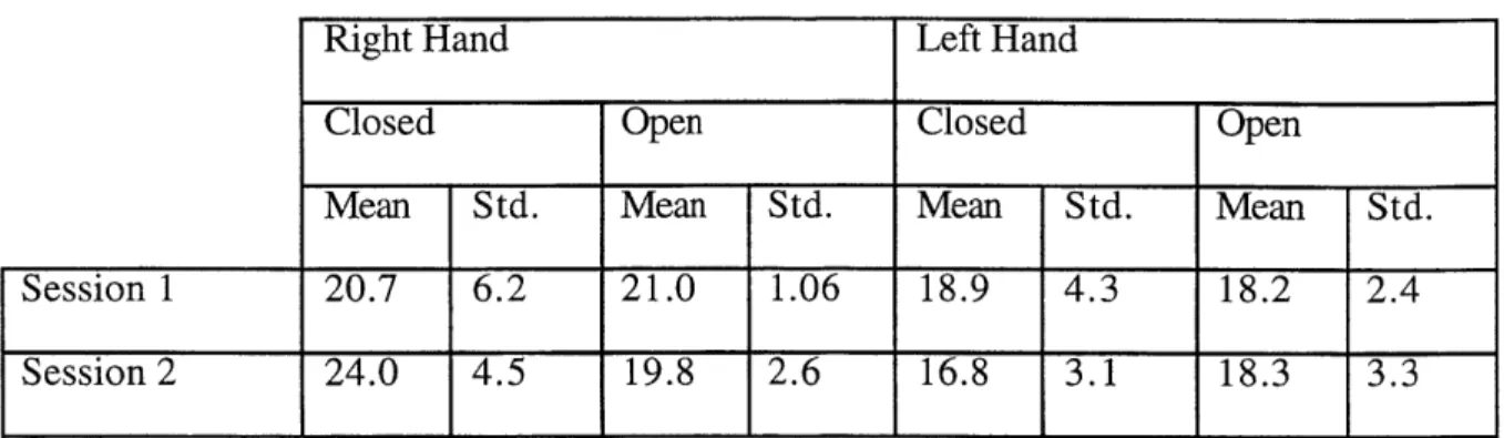
Data on wrist velocities is summarized in Table 4.1 and 4.2. While there does not

appear to be a pattern in the data pertaining to maximum wrist extension velocities, the

maximum wrist flexion velocities appear to be smaller for throws with eyes open in

general.

Table 4.1. Maximum Wrist Extension Velocity (cm/s)

Right Hand Left Hand

Closed Open Closed Open

Mean Std. Mean Std. Mean Std. Mean Std.

Session 1 45.2 3.0 49.2 5.6 53.9 1.2 48.2 3.8

Table 4.2. Maximum Wrist Flexion Velocity

Right Hand Left Hand

Closed Open Closed Open

Mean Std. Mean Std. Mean Std. Mean Std.

Session 1 20.7 6.2 21.0 1.06 18.9 4.3 18.2 2.4

Session 2 24.0 4.5 19.8 2.6 16.8 3.1 18.3 3.3

4.2. Elbow Motion

The elbow joint experiences both translation and rotation during a throw. The

transition is primarily the result of shoulder rotation which is not addressed in this analysis.

The elbow rotation causes the angle between the forearm and upper-arm to decrease during

flexion and increase during extension. Table 4.3. contains data for the maximum and

minimum angle (in degrees) of the elbow and their difference for each throw. "0" and "C" in the run number column indicate eyes open or closed, respectively. Also, throws made with the subject's right hand are marked "R" and those made left-handed are marked "L". The table shows that the subject started throws when he had his eyes closed with a wider elbow angle, and he extended his arm slightly more before releasing the ball on those throws. He also did not reach as small a minimum angle during flexion with eyes closed.

Despite these differences between throws made with eyes open and closed, the angle

between the subject's greatest flexion and extension was similar for both. This means the

subject traced out similarly sized trajectories for both types of throws, but the throws with

eyes open were performed closer to the body.

Table 4.3. Elbow Angle (degrees)

Session 1 Session 2

Minimum Maximum Difference Minimum. Maximum _Difference

R-C-1 69.9 100.6 30.7 67.2 98.0 30.8 R-C-2 61.3 92.1 30.8 66.4 107.5 41.1 R-C-3 55.2 94.0 38.8 60.1 99.2 39.1 R-C-4 55.5 97.2 41.7 48.9 94.0 45.1 R-C-5 61.4 95.0 33.6 55.8 91.2 45.4 R-O-1 62.2 100.4 38.2 50.1 92.5 41.4 R-O-2 58.1 95.9 37.8 44.9 89.6 44.7 R-O-3 61.9 91.7 29.8 49.3 94.7 45.4 R-O-4 56.2 99.1 42.9 47.1 89.8 42.8 R-0-5 62.4 96.3 33.9 52.1 91.4 39.3 L-C-1 60.5 99.9 39.4 66.5 96.9 30.4 L-C-2 60.4 103.3 42.9 53.0 90.6 37.6 L-C-3 62.6 102.8 40.4 61.4 92.1 30.7 L-C-4 54.0 96.1 42.1 61.2 93.3 31.4 L-C-5 67.7 106.3 38.6 61.0 95.2 34.2 L-O-1 57.1 93.2 36.1 52.9 91.9 39.0 L-O-2 53.2 91.8 38.6 65.1 100.3 35.3 L-O-3 47.4 93.3 45.9 55.7 94.0 38.3 L-O-4 56.8 94.8 38.0 59.9 97.6 37.7 L-O-5 50.4 91.6 41.2 64.2 101.7 37.6

Further examination of the elbow angle is achieved by plotting the angle vs. time. The elbow angle changes during the as throw shown in Figure 4.6. and 4.7. Figure 4.6

graphs the elbow angle (in degrees) for several throws made with eyes closed. In Figure 4.7., the throws from the previous graph are overlaid with the graphs of several throws made with eyes open. It is interesting to note that the throws made with eyes open are more consistent. The minima are closer to the same value and the shapes are more regular. In general, the curves are not symmetrical. The angle changes more gradually during the windup than it does during the extension of the arm. However, the curves become more symmetrical over time.

JL2RCo5.mat 110 00 90 80 70 -60 50 -40 -0 10 20 30 40 50 60

Fig. 4.6. Elbow Angle (degrees) v. Time for 5 throws, eyes closed. 1

JL2ROO5.mat 110 - 100-90 80 -70 -60 -50 -40 L 0 10 20 30 40 50 60

Fig. 4.7. Elbow angle v. Time, eyes closed and open.

4.3. Shoulder Motion

Since subjects were not restrained in shoulder harnesses, shoulder translation

occurred. The translation is summarized in Table 4.4. The values are small and do not

vary much. It is interesting to note that the values are more consistent for throws made

with closed eyes.

Table 4.4. Total Shoulder Translation [cm]

closed

Mean Standard D.

open

r.-.

Mean Standard V.

Session 1 Right Hand 2.68 .71 3.65 1.00

Left Hand 2.75 .77 2.79 .68

Session 2 Right Hand 2.38 1.37 1.92 .69

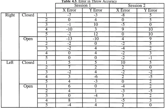
4.4. Throw Accuracy

Finally, Table 4.5. has been included to provide information on the errors in the subject's throwing accuracy. X and y errors are recorded in centimeters; the "bulls-eye" on the target was located at the origin of the x and y axes.

Table 4.5. Error in Throw Accuracy

Session 1 Session 2 Right Closed 1 -7 -3 -8 5 2 0 4 0 5 3 -1 10 -5 0 4 -10 3 9 10 5 -2 12 0 10 Open 1 -13 -10 4 9 2 -2 0 -2 5 3 -2 4 -4 2 4 0 4 -2 3 5 0 0 -2 -1 Left Closed 1 5 5 10 5 2 7 2 2 0 3 -2 4 -2 -2 4 3 -6 2 -5 5 4 -3 0 2 Open 1 6 0 -4 2 2 4 1 -3 -5 3 0 -4 3 2 4 8 1 -5 3 5 -4 4 2 0

5.

Discussion

The general limitations of the experiment are examined first. Then the implications

of the results are discussed and related to past experiments. The findings are then related to the aims of the experiment and explained. Finally, recommendations are made.

Some of the limitations of this experiment are the result of the difficulty in executing

it in the small volume available on Mir, others are the due to the way the raw data was

converted and analyzed. On Mir, the conditions were extremely cramped so that only one camera could be used resulting in 2 dimensional images of a 3-D process. In addition to

the size constraint, time pressures resulted in sessions being completed at irregular

intervals. In the data analysis, human error decreased the accuracy of manually registering

the joint markers (using a mouse) with Matlab. In addition, the joint markers (made of

duct-tape) were difficult to see. Finally, the large time required to process data resulted in

analysis of only a small number of trials. This means that it is not possible to reach solid

conclusions until more data is available.

This experiment examined the ways that astronauts adapt when exposed to a

microgravity environment. Specifically, it probed the kinematics of adaptive arm motions

for tossing a ball at a target. It is difficult to determine how much the subject in this

experiment experienced performance degradation upon entering microgravity since he did

not do trials on the ground and trials in space were not done at regular intervals. He was

reasonably well adapted to microgravity at the time of the trials for this experiment. He did

not exhibit any signs of perceptual difficulties (N.A.S., 1998) and performed the throwing

task well. It is unclear if the subject suffered from proprioceptive illusions (Cohen, 1970)

at the time of the trials; however, the fact that he did alter his throwing style in the absence

of visual feedback is suggestive that he did (Cohen, Welch, 1988). This style differed in

several ways with and without visual feedback. Most notably he reached out more toward

the target when his eyes were closed.

There were two significant differences in the subject's throwing style on the two

different days that he participated in the experiment. First, the peaks in the graphs of wrist

velocity and elbow angle became more symmetrical. This adaptation could be an example

of the subject adjusting to altered muscle loading in order to improve. Also, the wrist

trajectories became steeper. Since the targets were slightly lower than the subject's hand,

this indicates that the throws were becoming more direct. This adaptation could be the

result of the subject overcoming proprioceptive illusions, or the subject may simply have

needed to learn the novel task of throwing straight at the target instead of aiming a bit above

This experiment differed from most of those which studied adaptation of hand-eye coordination in microgravity (Bock, et al., 1992) in that it related to long-duration space flight. The subject did not exhibit large systematic errors in his aim. This reveals that once he was adapted to the microgravity environment learning new tasks was similar to doing so on Earth (N.A.S., 1998). The subject's neuromuscular motor control was adapted to microgravity (Cohen, 1970). This suggests that the learning curve for new tasks is reduced when astronauts are used to the space environment.

This experiment was just an introduction to this type of kinematic analysis

of long-duration space flight movement adaptations. The remaining data from this

experiment need to be analyzed and incorporated into this study. In addition, coordinating

the data collected by the EDLS sensors for each throw with the information already

available would produce interesting results whereby a dynamic astronaut model could be achieved by incorporating the arm kinematics with the ground reaction force data.

Future studies should include experimental test sessions earlier in the space

mission to capture the initial adaptation from 1-g to microgravity, and 3 dimensional

measurements would increase precision and reliability of kinematics data. Also, clearer

markers and better lighting conditions would make the data analysis easier and more accurate. The rest of the data from this experiment must be examined to confirm the initial findings. The information which is available from the EDLS sensors should be calibrated

and synchronized with the data from each throw.

6.

Conclusion

The kinematic analysis of arm throwing motions covered in this thesis suggested

several conclusions. First, the data from the sessions which have been analyzed so far

demonstrates that this experiment provides a useful way to measure some trends in

astronaut adaptation. The single subject studied appeared to adapt reasonably well to

problems as he adapted to space, and he adjusted some muscle usage to correct for

differences in muscle loading in microgravity. Overall, he performed the throwing task well and was consistent. It appeared that he still had some difficulty with his

proprioception; however, it was overcome easily when visual feedback was available. The

rest of the subjects will have to be analyzed and compared before these conclusions can be

generalized. Eventually, these observations may provide a basis for speculation as to the

Acknowledgments

This research effort was supported under NASA Contract NAS 1-18690. I would like to thank the astronaut subjects who participated in the experiment on MIR. I would also like to thank Mike Tryfonidis for his guidance and help with the data analysis process.

References

1. Abend, W., Bizzi, E., Morasso, P., "Human Arm Trajectory Formation,"

Brain, Vol. 105, 1982, pp.3 3 1-4 8.

2. Bock, 0., Howard, I. P., Money, K. E., Arnold K. E., "Accuracy of Aimed Arm Movements in Changed Gravity," Aviation Space and Environmental Medicine, Vol. 63, 1992, pp.9 9 4-8.

3. Cohen, M. M.,Welch R. B., "Hand-eye Coordination in Altered

Gravitational Fields," Aerospace Medicine, Vol. 41, 1970, pp.6 4 7-9.

4. Cohen, M. M.,Welch R. B., "Hand-eye Coordination During and After Parabolic Flight," Aviation Space and Environmental Medicine, Vol. 59,

1988, 474.

5. Gerathewohl, SJ., Strughold, H., Stallings, HD., Sensomotor Performance During Weightlessness: Eye-hand Coordination," J. Aviation Medicine, Vol.

28, 1957, pp.7-12.

6. Jackson, D.K., Development of Full-Body Models for Human Jump Landing Dynamics and Control. MIT Aeronautics and Astronautics S.D. Thesis, 1997.

7. Morasso, P., "Spatial Control of Arm Movements," Experimental Brain

Research, Vol. 42, 1981, pp.2 2 3-2 7.

8. National Academy of Sciences. Space Studies Board: Report of the Workshop on

Biology-based Technology to Enhance Human Well-being and Function in Extended Space Exploration, 1998.

9. Newman, D.J., Jackson, D.K., Bloomberg, J.J., "Altered astronaut lowerlimb and

mass center kinematics in downward jumping following space flight," Experimental Brain Research, Vol. 117, 1997, pp.3 0-4 2.

10. Newman, D.J., Tryfonidis, M., van Schoor, M.C., "Astronaut-Induced

Disturbances in Microgravity," Journal of Spacecraft and Rockets, Vol. 3 4, No. 2, March-April 1997, pp. 252-254.

11. Tryfonidis, M., Robust Adaptive Control Modeling of the Human CNS control of Arm Movements in conditions of Altered Gravity. MIT Aeronautic and Astronautics PhD

Thesis, 1998.

12. von Beckh, H. J. A., "Experiments with Animals and Human Subjects Under Sub- and Zero-gravity Conditions During the Dive and Parabolic Flight," J. Aviation Medicine, Vol. 25, 1954, pp.2 3 5-4 1.

13. Whiteside, TCD., "Hand-eye Coordination in Weightlessness," Aerospace

Medicine, Vol. 32, 1961, pp.3 18-2 2.

14. Young, L. R., Oman, C. N., Watt, D. G., Money, K. E., Lichtenberg, B. K., Kenyon, R. V. and Arrott, A. P., "M.I.T./Canadian Vestibular

Weightlessness and Readaptation to One-g: an Overview," Experimental Brain Research, Vol. 64, 1986, pp.291-8.

Appendix A

vidana.m

cle clf

clear functions

directory='This Directory Does NOT exist'; while exist(directory)-=7

directory=input('Enter the working directory: ','s');

clc end eval(['cd 'directory ""]); eval(['dir ' directory ".]); disp(") disp(") if exist('calibrate.mat')-=2

calibration file='This File Does NOT exist'; while exist(calibrationfile)==O

calibrationjfile=input('Enter the calibration file: ','s');

clc

end

eval(['[PIC,MAP]=imread("' calibrationfile ');']);

image(PIC) colormap(MAP)

disp('Now Pick The Origin of the Calibration Figure')

title('CALIBRATION -PICK THE ORIGIN')

[xcO,ycO]=ginput(1);

xcl=xcO; yc1=ycO;

while xci <=xcO

disp('Now Pick The X=+10cm point of the Calibration Figure')

title('CALIBRATION -PICK THE ORIGIN')

[xci,ycl]=ginput(1); end

xc2=xcO; yc2=ycO;

while yc2>=ycO

disp('Now Pick The Y=+1Ocm point of the Calibration Figure')

title('CALIBRATION -PICK THE ORIGIN')

[xc2,yc2]=ginput(1); end

xpixpercm=abs((xc1-xcO)/10); ypixpercm=abs((yc2-yc0)/1 0);

else

disp('It seems that there is already a calibration matrix for') disp('this series of images. Possibly some of the images have') disp('already been analyzed and logged.')

load calibrate

end

disp(")

disp('[PLEASE, PRESS ANYKEY TO CONTINUE!]') pause

clc

currentfile='This File Does NOT exist'; while exist(currentfile)-=2

eval(['dir ' directory ""]);

currentfile=input('Now, enter the first file to analyze: ','s'); if length(current file)==O

currentfile='This File Does NOT exist'; end clc end currentfile=[current-file blanks(80-length(current-file))]; lcf=80; for counter=80:- 1:1 junk=blanks(80-counter+1); if currentfile(counter:80)==junk lcf=counter- 1; end end FILES=[blanks(80)];

while eval(['exist(' current_file(1:lcf) ')'])==2 1 currentfile-=['O' blanks(79)]

cle

markerl=[]; counter=[]; fileexist=[];

while (file-exist ~='y') & (file-exist ='n') eval(['dir "' directory ""]);

datafile = current file(1:9)

file-exist=input('does this file exist in this directory? (y/n): ','s'); end

if fileexist=='y'

eval([' load 'data__file ""])

junk=size(FILES); datafilejlength=junk(1);

for counter= 1:datafilelength

if FILES(counter,:)==currentfile disp('This File has been Analyzed before!') markerl=counter;

end if isempty(markerl)==1 marker 1 =datafilejlength+1; end else files=[blanks(80)]; markerl=1; end markerl1 pause clf eval(['[PIC,MAP]=imread("' current-file(1:lcf) .');']); image(PIC) colormap(MAP) title(current-file(1:lcf))

disp('Enter the sensor to joint marker to read:')

sensor=input('1:SHOULDER / 2:ELBOW / 3:WRIST / 0:DONE >';

clear XSl XS2 XS3 YS1 YS2 YS3

while sensor-=0 if sensor== 1 [XS1,YS1]=ginput(1); hold on xtemp=[]; ytemp=[]; xtemp=[XS1-10:0.1:XS1+10];

ytemp=real(sqrt( 10A2-(xtemp-XS 1).A2));

plot(xtemp,YS 1 -ytemp) plot(xtemp,YS 1 +ytemp) end if sensor==2 [XS2,YS2]=ginput(1); hold on xtemp=[]; ytemp=[]; xtemp=[XS2-10:0.1:XS2+10]; ytemp=real(sqrt( 10A2-(xtemp-XS2).A2)); plot(xtemp,YS2-ytemp) plot(xtemp,YS2+ytemp) end if sensor==3 [XS3,YS3]=ginput(1); hold on xtemp=[]; ytemp=[]; xtemp=[XS3-10:0.1:XS3+10]; ytemp=real(sqrt( 1 0A2-(xtemp-XS3).A2)); plot(xtemp,YS3-ytemp) plot(xtemp,YS3+ytemp) end

disp('Enter the sensor to joint marker to read:')

sensor=input('1:SHOULDER / 2:ELBOW / 3:WRIST I 0:DONE >');

while sensor==0 & (exist('XS1')-=1 I exist('XS2')-=1 I exist('XS3')-=1)

clc

disp('You have not yet finished with ALL the joints!') disp('Enter the sensor to joint marker to read: ')

end end

FILES (marker 1,:)=currentfile;

X_SHOULDER(markerl ,1 )=(XS 1);YSHOULDER(markerl, 1)=(-YS 1); X_ELBOW(markerl,1)=(XS2);YELBOW(markerl,1)=(-YS2);

X_WRIST(markerl,l)=(XS3);YWRIST(markerl,1)=(-YS3);

eval(['save ' datafile' FILES XSHOULDER XELBOW XWRIST YSHOULDER

Y_ELBOW YWRIST']); clc clear suggestfile junk= ['000' num2str(str2num(current_file(lcf-3 :lcf))+ 1)]; suggest-file=[current_file(1:lcf-4) junk(length(junk)-3:length(junk)) currentfile(lcf+1:80)]; dir if exist(suggest-file(1:lcf))==2

disp(['Default Next File: ' suggestjfile(1:lcf)]) disp('Enter 0 to QUIT.')

else

disp('Default is to QUIT.') suggest-file=['0' blanks(79)]; end

temp-file=input('Now, enter the NEXT file to analyze: ','s'); if isempty(temp-file)==1 currentfile=suggestfile; else if exist(temp-file)==2 current-file=[tempfile blanks(80-lcf)]; else current-file=['O' blanks(79)]; end end end

Appendix B

wristvelocity.m

clc clf

clear functions

filler = [nan nan nan nan nan nan nan nan nan nan nan nan nan nan nan nan nan nan nan nan nan nan nan nan nan nan nan nan nan nan nan nan nan nan nan nan nan nan nan nan nan nan nan nan nan nan nan nan nan nan nan nan nan nan nan nan nan nan nan nan]; bigmatrix = [filler', filler', filler', filler', filler'];

directory='This Directory Does NOT exist'; while exist(directory)-=7

directory=input('Enter the working directory: ','s');

cle

end

eval(['cd "'directory ""]);

disp(") disp(")

% check if calibration file exists

if exist('calibrate.mat')-=2

calibration file='This File Does NOT exist'; while exist(calibrationfile)==O

calibrationjfile=input('Enter the calibration file: ','s');

clC

end

load calibrate % load calibration file

else load calibrate end disp(") disp('[PLEASE, pause

PRESS ANYKEY TO CONTINUE!]')

for plotplace = 1:5

cle

currentfile='This File Does NOT exist';

while exist(current-file)-=2 % check if datafile exists

eval(['dir ' directory ""]);

currentfile=input('Now, enter the first file to analyze: ','s'); if length(currentjfile)==O

end

clc

end

eval([' load "'current-file ""]) % load datafile

%create time matrix

FRAMES = [0:(1/30):1.9667]; % create calibrated variables

X_S = (XSHOULDER/xpixpercm); Y_S = (YSHOULDER/ypixpercm); X_E = (XELBOW/xpixpercm); Y_E = (YELBOW/ypixpercm); X_W = (XWRIST/xpixpercm); Y_W = (YWRIST/ypixpercm); X_Wcal = XW -min(XW);

%plot wrist position figure(1) subplot(3, 5, plotplace) plot(X_WcalY_W,'-') hold on %TITLE('WRIST POSITION') if plotplace ==1 title('JL2-RC-01') elseif plotplace == 2 title('JL2-RC-02') elseif plotplace == 3 title('JL2-RC-03') elseif plotplace == 4 title('JL2-RC-04') else title('JL2-RC-05') end axis('equal') axis([O 15 -40 -20]) %XLABEL('x (cm)') %YLABEL('y (cm)') figure(1) subplot(3, 5, plotplace + 5) hold on axis([0 60 0 15]) axis('normal') plot(XWcal, '-m')

%TITLE('Wrist position v. time (x compontent)') %title(eval(['current file'])) %

figure(1)

subplot(3, 5, plotplace + 10) hold on

axis([0 60 -42 -26]) axis('normal') plot(YW, 'g')

%TITLE('Wrist position v. time (y component)') %title(eval(['current file'])) % %run wristdist X_Wi = X_W; lenXW = length(XW); X_Wi([ eval(['lenXW'])

])

deltaYW = (Y_Wf -Y_Wi);

%plot wrist velocity figure(3) %subplot(5, 1, plotplace) hold on lenDXW = length(deltaXW); Frames = FRAMES; Frames([ eval(['lenDXW']) + 1:60]) = %plot(Frames, deltaXW, ':') lenDYW = length(deltaYW); Frames = FRAMES; Frames([ eval(['lenDYW']) + 1:60]) = %plot(Frames, deltaYW, '--g')

deltaXW = abs(XWf -XWi);

deltaYW = abs(YWf -YWi);

cWsquared = ((deltaXW).A2) + ((deltaYW).A2); deltaWpos = []

smoothdeltang =

lenDWP = [];

lenDWP = length(deltaWpos);

for ind = 1:lenDWP

if ind == 1

smoothdeltang(1) = (deltaWpos(1) + deltaWpos(2))/2;

elseif ind == lenDWP

%do nothing else

smoothdeltang(ind) = (deltaWpos(ind) + deltaWpos(ind + 1))/2;

end end lenDWP = length(deltaWpos); Frames = FRAMES; %Frames([ eval(['smoothdeltang']) + 1:60]) = endder=length(smoothdeltang);

[thenum, spot] = max(smoothdeltang); wristspeed = thenum * 30;

diffs = 45 -spot; for indo = 1:endder

littlematrix(plotplace) = wristspeed; if diffs > 0

bigmatrix(indo + diffs, plotplace) = [smoothdeltang(indo)]; else

bigmatrix(indo, plotplace) = [smoothdeltang(indo)]; end

end

diffsmult = diffs * FRAMES(2);

Frames = FRAMES + diffsmult;

Frames([ length(smoothdeltang) + 1:60

])=

plot( Frames, smoothdeltang) axis('normal') axis([0 2 0 2]) TITLE('Wrist Velocity') eval(['current file']) %title(eval(['current file'])) %XLABEL('Time (s)')

%YLABEL('Change in Wrist Position (cm)')

%wrist acceleration %run wristacc

deltaXWi = deltaX_W;

lendeltaXW = length(deltaXW);

deltaXWf = deltaXW; deltaXWf(1) = []; deltaYWi = deltaY_W; lendeltaYW = length(deltaYW); deltaYWi([ eval([lendeltaYW'])

])

delta2XW = (deltaXWf - deltaXWi);

delta2YW = (deltaYWf - deltaYWi);

%plot wristacc %figure %(4) %subplot(5, 1, plotplace) hold on lenD2XW = length(delta2XW); Frames = FRAMES; Frames([ eval(['lenD2XW']) + 1:60

])

delta2XW = abs(deltaXWf -deltaX Wi);

delta2YW = abs(deltaYWf - deltaYWi);

cWsquared2 = ((delta2XW).A2) + ((delta2YW).A2);

deltaWpos2 = sqrt(cWsquared2); lenDWP2 = length(deltaWpos2); Frames = FRAMES; Frames([ eval(['1enDWP2']) + 1:60]) =

[1;

%YLABEL('Change in Wrist Velocity (cm)')

end figure(3)

Ibm = length(mean(bigmatrix')); Frames([ (ibm + 1):60 1) = [];

plot(Frames, mean(bigmatrix'), 'in')

title('Average Wrist Velocity') XLABEL('Time (s)')

YLABEL('Change in Wrist Position (cm)') littlematrix mean(littlematrix) std(littlematrix)

elbowangle.m

directory='This Directory Does NOT exist'; while exist(directory)-=7

directory=input('Enter the working directory: ','s');

clc

end

eval(['cd "'directory ""]);

disp(") disp(")

% check if calibration file exists

if exist('calibrate.mat')-=2

calibration file='This File Does NOT exist'; while exist(calibration-file)==0

calibrationfile=input('Enter the calibration file: ','s');

clc

end

load calibrate % load calibration file

else

load calibrate

end

disp(")

disp('[PLEASE, PRESS ANYKEY TO CONTINUE!]') pause

for

j=1:10

currentfile='This File Does NOT exist';

eval(['dir .' directory ""]);

currentfile=input('Now, enter the first file to analyze: ','s'); if length(currentjfile)==O

currentfile='This File Does NOT exist'; end

clc

end

eval([' load "'currentfile ""]) % load datafile

%create time matrix

FRAMES = [0:(1/30):1.9667];

% create calibrated variables

XS = (X_SHOULDER/xpixpercm); YS = (YSHOULDER/ypixpercm); XE = (X_ELBOW/xpixpercm); YE = (YELBOW/ypixpercm); X_W = (XWRIST/xpixpercm); Y_W = (YWRIST/ypixpercm);

% make new matrix

Y_F = abs(YW - YE);

X_F = abs(XW - XE);

FANGLE = atan(XF ./ YF);

FANGDEG = FANGLE .* (180/pi); Y_U = abs(YE - YS);

X_U = abs(XE - XS); UANGLE = atan(X_U ./ YU); UANGDEG = UANGLE .* (180/pi);

ELBOWANGLE = (FANGDEG + UANGDEG)

minangle = min(ELBOWANGLE)

maxangle = max(ELBOWANGLE);

anglediff = (max-angle -min-angle) eval(['current_file'])

lenelbang = length(ELBOWANGLE)

minisat = []

for indi = 1:lenelbang

if ELBOWANGLE(indi) == minangle a=2 minisat = indi end end =

disttomove = 45 - minisat end

y = [(distjto_move + 1):(disttomove + lenelbang)]

ifj==1 plot(y,ELBOWANGLE, 'ob-') elseif j==2 plot(y,ELBOWANGLE, 'xb-') elseif j==3 plot(y,ELBOWANGLE, '+b-') elseif j==4 plot(y,ELBOWANGLE, 'vb-') elseif j==5 plot(y,ELBOWANGLE, 'sb-') elseif j==6 plot(y,ELBOWANGLE, 'om-') elseif j==7 plot(y,ELBOWANGLE, 'xm-') elseif j==8 plot(y,ELBOWANGLE, '+m-') elseif j==9 plot(y,ELBOWANGLE, 'vm-') else plot(y,ELBOWANGLE, 'sm-') end axis([0 60 40 110]) title(eval(['currentfile'])) hold on %phase-plane diagram DELTAELBANG = diff(ELBOWANGLE); len-elb-ang = length(ELBOWANGLE);

for ind = 1:lenelbang if ind == 1

smoothelbowang(1) = (ELBOWANGLE(1) + ELBOWANGLE(2))/2;

elseif ind == lenelbang

%do nothing else

smoothelbowang(ind)= (ELBOWANGLE(ind) + ELBOWANGLE(ind +

1))/2; end end %figure %plot(smoothelbowang) end

Appendix C

This appendix contains graphs of the wrist trajectories for all of the throws analyzed in this thesis. The graphs in the top row of each set show the path that the wrist followed

during a throw. Both axes are in divided into centimeters. The two graphs directly under

those present the x and y position of the wrist v. time, respectively. The axes are measured

in centimeters and seconds. Each set of 5 graphs is a group was done with the same hand and eye conditions. Throws titled "JL2" were executed on March 6,1997 and those titled

"JL4" on March 26, 1997. "R" and "L" refer to the hand used, and "C" and "0" indicate

the eye condition.

JL2-RC-01 JL2-RC-02 JL2-RC-03 JL2-RC-04 JL2-RC-05 -20 . -20 . -20 . -20 . -20 -25 -25 -25 -25 -25 -30 -30 -30 -30 .-30 -35 -35 -35 -35 -35 -40 -40 140 . 1-40 .40 0 5 10 15 0 5 10 15 0 5 10 15 0 5 10 15 0 5 10 15 15 15 15 15 15 10 10 10 10 10 5 .5 5 5 5 0 0 0 0 0 0 50 0 50 0 50 0 50 0 50 -30 -30 -30 -30 ^ -30 -35 -35 --35 -35 -35 -40 -40 -40 -40 -40 0 50 0 50 0 50 0 50 0 50

JL2-RO-01 JL2-RO-02 JL2-RO-03 JL2-RO-04 JL2-RO-05 -20 -20 -20 -20 -20 -25 -25 -25 -25 -25 -30 -30 -30 -30 -30 -35 -35 -35 -35 -35 -40 -40 -40 -40 -40 0 5 10 15 0 5 10 15 0 5 10 15 0 5 10 15 0 5 10 15 15 15 15 15 15 10 10 10 10 10 5 5 5 5 5/ II 0 0 0E 0 0 0 50 0 50 0 50 0 50 0 50 -30 -30 -30 -30 -30 -35 ... - -35 -35 -40 -40 -40 -40 -40 0 50 0 50 0 50 0 50 0 50 JL2-LC-01 JL2-LC-02 JL2-LC-03 JL2-LC-04 JL2-LC-05 -20 -20 -20 -20 -20 -25 -25 -25 -25 . -25 -30 -30 -30 -30 -30 -35 -35 -35 -35 -35 -40 -40 -40 -40 -40 0 5 10 15 0 5 10 15 0 5 10 15 0 5 10 15 0 5 10 15 15 15 15 15 15 10 10 10 10 10 5 5 5 5 0 - 010 - 0 0 0 50 0 50 0 50 0 50 0 50 -30 -30 -30 -30 -30 -35 -35 -35 -35 -35 -40 -40 -40 -40 -40 0 50 0 50 0 50 0 50 0 50

JL2-LO-01 JL2-LO-02 JL2-LO-03 JL2-LO-04 JL2-LO-05 -20 -20 -20 -20 -20 -25 -25 -25 -25 -25 -30 -30 -30 -30 -30 -35 -35 -35 -35 -35 -40 -40 -40 -40 -40 0 5 10 15 0 5 10 15 0 5 10 15 0 5 10 15 0 5 10 15 15 15 15 15 15 10 10 10 10 10 5 5 5 5 5 0 0 0 . 0 0-0 50 0 50 0 50 0 50 0 50 -30 .s -30 -30 -30 -30 -35 -35 -35 -35 -35 -40 -40 -40 -40 -40 0 50 0 50 0 50 0 50 0 50 JL4-RC-01 JL4-RC-02 JL4-RC-03 JL4-RC-04 JL4-RC-05 -20 -20 -20 -20 -20 -25 -25 -25 -25 -25 -30 -30 -30 -30 -30 -35 -35 -35 -35 -35 -40 -40 -40 -40 -40 0 5 10 15 0 5 10 15 0 5 10 15 0 5 10 15 0 5 10 15 15 15 15 15 15 10 10 10 10 10 5 5 5 5 5 0 0 0 0 0 0 50 0 50 0 50 0 50 0 50 -30 -30 -30 -30 -30 -35 JE, f7> -3 -35 -35 -35 ...---...'..35 -40 -40 -40 -40 - -40 0 50 0 50 0 50 0 50 0 50

JL4-RO-01 JL4-RO-02 JL4-RO-03 JL4-RO-04 JL4-RO-05 -20 -20 -20 -20 -20 -25 -25 -25 -25 -25 -30 -30 -30 -30 -30 -35 -35 -35 -35 -35 -40 -40 -40 -40 -40 0 5 10 15 0 5 10 15 0 5 10 15 0 5 10 15 0 5 10 15 15 15 15 15 15 10. 10 10 10 10 5 5 5 5 5 0- 0- 0 0- 0-0 50 0 50 0 50 0 50 0 50 -30 -35 -40 0 50 -30 -30 -30 -35 -35 -35 -40 -40 -40 0 50 0 50 0 50 -30 -35 -40 0 50 JL4-LC-01 JL4-LC-02 JL4-LC-03 JL4-LC-04 JL4-LC-05 -20 -20 -20 -20 -20 -25 -25 -25 -25 -25 -30 -30 -30 -30 -30 -35 -35 -35 -35 -35 -40 -40 -40 -40 -40 0 5 10 15 0 5 10 15 0 5 10 15 0 5 10 15 0 5 10 15 15 15 15 15 15 10 10 10 10 10 5 5 5 - 5 5-0 0 0 o 0 0 50 0 50 0 50 0 50 0 50 -30 -35 -40 0 50 -30 <'~ -30 -35 -35 -40 -40 0 50 0 50 -30 -35 -40 0 50 -30 -35 -40 0 50

JL4-LO-01 JL4-LO-02 JL4-LO-03 JL4-LO-04 JL4-LO-05 -20 -20 -20 -20 -20 -25 -25 -25 -25 -25 -30 -30 -30 -30 -30 -35 -35 -35 -35 -35 -40 -40 -40 -40 -40 0 5 10 15 0 5 10 15 0 5 10 15 0 5 10 15 0 5 10 15 15 15 15 15 15 10 10 10 10 10 5 5- 5 5 5 0 0 0 0 0 0 50 0 50 0 50 0 50 0 50 -30 -30 -30 -30 -30 -35 -35 ^.. ... -35 -35 -.-- -35 -40 -40 -40 -40 -40 0 50 0 50 0 50 0 50 0 50