HAL Id: hal-00951800
https://hal.archives-ouvertes.fr/hal-00951800
Submitted on 10 Jul 2020
HAL is a multi-disciplinary open access
archive for the deposit and dissemination of
sci-entific research documents, whether they are
pub-lished or not. The documents may come from
teaching and research institutions in France or
abroad, or from public or private research centers.
L’archive ouverte pluridisciplinaire HAL, est
destinée au dépôt et à la diffusion de documents
scientifiques de niveau recherche, publiés ou non,
émanant des établissements d’enseignement et de
recherche français ou étrangers, des laboratoires
publics ou privés.
The seasonal variation of the CO2 flux over Tropical
Asia estimated from GOSAT, CONTRAIL and IASI
Sourish Basu, M. Krol, A. Butz, Cathy Clerbaux, Y. Sawa, T. Machida, H.
Matsueda, C. Frankenberg, O. P. Hasekamp, I. Aben
To cite this version:
Sourish Basu, M. Krol, A. Butz, Cathy Clerbaux, Y. Sawa, et al.. The seasonal variation of the CO2
flux over Tropical Asia estimated from GOSAT, CONTRAIL and IASI. Geophysical Research Letters,
American Geophysical Union, 2014, 41 (5), pp.1809-1815. �10.1002/2013GL059105�. �hal-00951800�
RESEARCH LETTER
10.1002/2013GL059105 Key Points:
• GOSAT estimates a dynamic seasonal cycle over Tropical Asia
• The GOSAT-estimated seasonal cycle is confirmed by CONTRAIL data • IASI CO shows that the dynamism is
not caused by biomass burning
Supporting Information: • Readme • Text S1 Correspondence to: S. Basu, sourish.basu@noaa.gov Citation:
Basu, S., M. Krol, A. Butz, C. Clerbaux, Y. Sawa, T. Machida, H. Matsueda, C. Frankenberg, O. P. Hasekamp, and I. Aben (2014), The seasonal variation of the CO2flux over Tropical Asia esti-mated from GOSAT, CONTRAIL, and IASI, Geophys. Res. Lett., 41, 1809–1815, doi:10.1002/2013GL059105.
Received 20 DEC 2013 Accepted 21 FEB 2014
Accepted article online 24 FEB 2014 Published online 12 MAR 2014
The seasonal variation of the CO
2
flux over Tropical Asia
estimated from GOSAT, CONTRAIL, and IASI
S. Basu1,2,3, M. Krol1,3,4, A. Butz5, C. Clerbaux6, Y. Sawa7, T. Machida8, H. Matsueda7,
C. Frankenberg9, O. P. Hasekamp1, and I. Aben1
1SRON Netherlands Institute for Space Research, Utrecht, Netherlands,2National Oceanic and Atmospheric Administration, ESRL/GMD, Boulder, Colorado, USA,3Institute for Marine and Atmospheric Research Utrecht, Utrecht University, Utrecht, Netherlands,4MAQ, Wageningen University and Research Centre, Wageningen, Netherlands, 5IMK-ASF, Karlsruhe Institute of Technology, Eggenstein-Leopoldshafen, Germany,6UPMC University Paris 06, Université de Versailles Saint-Quentin-en-Yvelines, CNRS/INSU, LATMOS-IPSL, Paris, France,7Meteorological Research Institute, Tsukuba, Japan,8National Institute for Environmental Studies, Tsukuba, Japan,9Jet Propulsion Laboratory, California Institute of Technology, Pasadena, California, USA
Abstract
We estimate the CO2flux over Tropical Asia in 2009, 2010, and 2011 using Greenhouse Gases Observing Satellite (GOSAT) total column CO2(XCO2) and in situ measurements of CO2. Compared to flux estimates from assimilating surface measurements of CO2, GOSAT XCO2estimates a more dynamic seasonal cycle and a large source in March–May 2010. The more dynamic seasonal cycle is consistent with earlier work by Patra et al. (2011), and the enhanced 2010 source is supported by independent upper air CO2 measurements from the Comprehensive Observation Network for Trace gases by Airliner (CONTRAIL) project. Using Infrared Atmospheric Sounding Interferometer (IASI) measurements of total column CO (XCO), we show that biomass burning CO2can explain neither the dynamic seasonal cycle nor the 2010source. We conclude that both features must come from the terrestrial biosphere. In particular, the 2010 source points to biosphere response to above-average temperatures that year.
1. Introduction
Seasonal variation in the land-atmosphere CO2flux is caused by the changing balance between
ecosys-tem productivity and respiration and by seasonal biomass burning. Therefore, interannual variations in the CO2flux reflect year to year differences in the ecosystem response to weather and anomalous climate
events such as high temperatures and low rainfall resulting in large-scale seasonal anomalies in CO2fluxes [Gatti et al., 2014]. Assessing the interannual variability of seasonal fluxes could therefore lead to better understanding of the response of the terrestrial ecosystem to climate variability and extreme events. Till recently, top-down estimates of seasonal fluxes relied solely on observed gradients of near-surface dry air CO2mole fractions. Rayner and O’Brien [2001] demonstrated the potential added value of global total
col-umn CO2(XCO2) measurements for obtaining better CO2flux estimates. The Greenhouse Gases Observing
Satellite (GOSAT) was launched in 2009 to provide global measurements of XCO2[Kuze et al., 2009].
Atmospheric inversion of GOSAT XCO2to estimate surface fluxes, however, has proved challenging, since
measurement biases as small as 0.5 ppm significantly affect the derived fluxes at regional scales [Basu et al., 2013; Chevallier et al., 2007]. Since GOSAT XCO2biases have no known year to year variations, multiyear anal-ysis of fluxes over a single region suffers less from such biases [Guerlet et al., 2013a]. In this manuscript, we analyze the seasonal cycle in the CO2flux from Tropical Asia derived from surface and GOSAT observations.
In section 2, we present flux estimates over Tropical Asia and validate them by comparing our posterior CO2
fields with Comprehensive Observation Network for Trace gases by Airliner (CONTRAIL) data in section 3. In sections 4 and 5 we estimate the biomass burning contribution to the seasonal cycle seen in section 2 by assimilating Infrared Atmospheric Sounding Interferometer (IASI) total column CO (XCO) [George et al., 2009] and using known CO:CO2emission ratios [Christian et al., 2003]. Finally, in section 6 we examine temperature
anomalies over Tropical Asia and GOSAT-derived chlorophyll fluorescence [Frankenberg et al., 2011] to deter-mine whether the land biosphere could be responsible for variations not explained by biomass burning in section 5.
Geophysical Research Letters
10.1002/2013GL059105
Figure 1. Monthly mean GOSAT XCO2(red diamonds) and cosampled modeled XCO2corresponding to surface fluxes optimized with surface CO2measurements (blue circles), after subtracting the same linear trend from both time series. Only measurements around Tropical Asia were considered for this plot, although for the flux inversion all measurements were used.
2. CO
2Flux Estimates Over Tropical Asia
We estimate the CO2flux over Tropical Asia by assimilating both surface observations of CO2and RemoTeC
v2.11 retrievals of GOSAT XCO2[Butz et al., 2009] in a four-dimensional variational (4DVAR) atmospheric
inversion using the atmospheric tracer transport model TM5 [Krol et al., 2005]. Monthly fluxes over the period 1 March 2009 to 1 October 2011 are estimated for 6◦× 4◦grid cells globally and subsequently aggre-gated over Tropical Asia over 3 month time periods. The inversion system and data streams are exactly as described in detail by Basu et al. [2013], with the following modification. Guerlet et al. [2013b] showed that RemoTeC XCO2retrieved from GOSAT soundings over land (acquired in high-gain mode) had biases dependent on the retrieved aerosol parameters, the strongest component being a linear dependence on the inverse of the retrieved aerosol size parameter as[Butz et al., 2009]. Combined with the overall land-sea offset discussed by Basu et al. [2013], this resulted in the following bias correction for GOSAT XCO2:
XCO2(ocean)→ XCO2(ocean) + b1 XCO2(land)→ XCO2(land) ×
(
b2+ b3 as
) (1)
Starting from the prior values given by Guerlet et al. [2013b], the inversion estimates the parameters b1, b2,
and b3simultaneously with the surface CO2flux from the land biosphere and the oceans. Fossil fuel and fire
emissions are imposed but not optimized.
Figure 1 shows monthly average GOSAT XCO2within (10◦S, 28◦N) and (80◦E, 156◦E)—a rectangular region
which covers Tropical Asia—during the inversion period (red diamonds). A linear trend of 2.11 ppm/yr was subtracted from the XCO2data. The trend was calculated by considering GOSAT XCO2soundings in the southern extratropics with yearlong coverage, i.e., within 35◦S and 23.5◦S over 3 years since the start of the GOSAT data stream in June 2009. Also shown in Figure 1 is the posterior atmospheric XCO2field from an inversion with only surface data, cosampled with GOSAT soundings (blue circles). We see that GOSAT XCO2 shows a more dynamic seasonal cycle compared to what a surface-only inversion would estimate. While it is not straightforward to link differences in measurement to differences in surface flux due to atmospheric transport, we can expect the seasonal cycle amplitude of the surface flux from a surface-only inversion to increase if GOSAT XCO2were assimilated in tandem.
Figure 2 shows the estimated CO2emissions—minus the fossil fuel component—over Tropical Asia. Since
GOSAT started its regular data stream in June 2009, the flux aggregate for March–May (MAM) 2009 is only marginally affected by GOSAT XCO2and is not considered hereafter. Over the rest of the inversion period, as
expected from the observations in Figure 1, the joint inversion predicts a noticeably more dynamic seasonal cycle compared to either a surface-only inversion or the prior flux estimate. Moreover, the joint inversion also predicts more outgassing of CO2during MAM 2010. As shown by Guerlet et al. [2013a], a sparse surface network might easily miss such a flux anomaly (only 270 of the 28,111 surface measurements assimilated are in or immediately downstream of Tropical Asia). To validate this anomaly, we compare our atmospheric CO2fields (corresponding to optimized fluxes) with CONTRAIL measurements of CO2above this area. Since
Figure 2. Surface CO2flux per 3 month time window from Tropi-cal Asia (red-shaded region in the inset). The fossil fuel flux has been subtracted. The time period prior to a steady GOSAT data stream is crosshatched. “Prior” refers to the prior emissions (a combination of Global Fire Emissions Database version 3.1 (GFED3.1) biomass burn-ing and Carnegie-Ames-Stanford approach (CASA) GFED biosphere flux), “Surface” refers to an inversion using only surface CO2 observa-tions, and “Surface + GOSAT” refers to a joint GOSAT XCO2and surface CO2assimilation. The time series “Prior (BB adj)” is the prior flux with a different estimate of the biomass burning CO2flux as explained in section 5.
the Tropics are a region of deep convection, we expect to see some of this outgassing signal in the free troposphere.
3. Verification With
CONTRAIL CO
2The CONTRAIL project [Machida et al., 2008] has been observing vertical CO2
profiles over 43 airports worldwide and along intercontinental flight paths using five Japan Airlines commercial airliners. The data coverage is extensive in the Northern Hemisphere, and vertically the samples go up to 150 hPa [Sawa
et al., 2012]. Niwa et al. [2012]
demon-strated that due to deep convection over the Tropics, CONTRAIL measurements impose strong constraints on terrestrial fluxes from Tropical Asia. Therefore, we use CONTRAIL measurements of CO2to
evaluate which of the (optimized) flux scenarios in Figure 2 is the most realistic. We sample our posterior atmospheric CO2fields from both the surface-only and joint inversions at CONTRAIL sample locations between 5 km and
13 km, 10◦S and 28◦N latitudes, 80◦E and 156◦E longitudes and present monthly average observed and modeled CO2values in Figure 3.
We see that from June 2009 (when the GOSAT data record started), the joint inversion better matches CONTRAIL observations. This is to be expected, since unlike surface measurements, GOSAT XCO2contains
information about the free and upper troposphere, which is what CONTRAIL samples. Figure 3 also shows that CONTRAIL measurements in April–June 2010 are ∼1 ppm higher than predicted by a surface inversion and are matched very well by the joint inversion. Since 349,921 of the 397,759 CONTRAIL measurements used here were taken above 10 km, this 1 ppm signal is present in the upper troposphere, which must cor-respond to a significant source at the surface. Therefore, the CO2source seen by CONTRAIL in spring 2010
(Figure 3) is consistent with the source estimated by GOSAT XCO2(Figure 2) over the same period. The
enhanced drawdown in September–November (SON) 2010 estimated by GOSAT (Figure 2) is seen to a lesser extent in the CONTRAIL data in Figure 3, while the enhanced source in MAM 2011 seen in the CONTRAIL data is not reproduced by the GOSAT inversion, likely due to the inversion ending in September 2011. The enhanced seasonal cycle and the 2010 spring source has to be due either to biomass burning or the land biosphere. Although the prior estimates a higher source in 2010 compared to neighboring years, it is possible that that is still an underestimation. To get an independent handle on biomass burning CO2flux
over this region, we assimilate XCO measurements from the IASI instrument on board the Meteorological Operational A (MetOp-A) satellite [Fortems-Cheiney et al., 2009] in a 4D VAR CO inversion.
4. CO Flux Estimate From Biomass Burning
The CO total column data used in this study were retrieved using the FORLI-CO algorithm [Hurtmans et al., 2012]. Daily data are available from the Ether database (http://www.pole-ether.fr). The CO inversion frame-work is identical to that described by Krol et al. [2013], with the following differences. We run the TM5 atmospheric transport model [Krol et al., 2005] at 6◦× 4◦resolution globally, at 3◦× 2◦resolution within (10◦S–42◦N, 54◦E–138◦E), and at 1◦× 1◦resolution within (2◦S–34◦N, 66◦E–126◦E). Within the 1◦× 1◦and 3◦× 2◦regions, we optimize biomass burning CO flux with a 3 day time resolution and impose monthly
Geophysical Research Letters
10.1002/2013GL059105
Figure 3. Comparison of monthly mean CONTRAIL CO2measurements and cosampled posterior CO2fields from our inversions. The hatched region represents the period before the start of the GOSAT data stream. Red points in the inset represent CONTRAIL measurements which were used to construct this plot, whereas blue dots represent surrounding measurements which were not used.
natural and anthropogenic emissions, as well as CO production from hydrocar-bons such as CH4. To provide boundary
conditions consistent with CO sampled by the NOAA flask sampling network [Novelli and Masarie, 2013], we addition-ally optimize weekly total CO emissions in the 6◦ × 4◦region. The biomass burning emissions are given a prior cor-relation length (exponential) of 200 km and a prior correlation time (exponential) of 3 days, whereas for the total emission in the 6◦× 4◦region those numbers are 1000 km and 15 days, respectively. This allows the inversion system maxi-mum flexibility to fit localized, short-term biomass burning events within the area of interest (Tropical and South Asia), while creating a smoother adjust-ment of the background outside the 3◦× 2◦region.
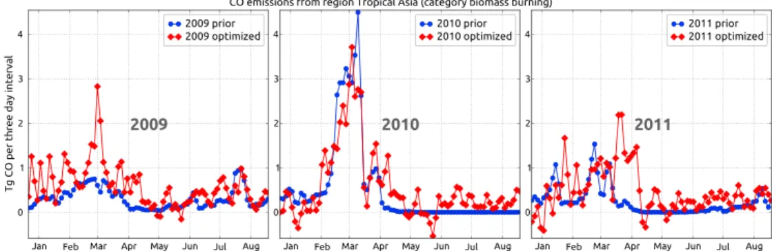
We performed three 10 month inversions from 1 December, year Y to 1 October, year Y + 1, where Y stands for 2008, 2009, and 2010. In each case, the starting CO fields on 1 December were created by running 4 month inversions with exactly the same setup from 1 August to 1 December of the corresponding year. The optimized biomass burning CO emissions, aggregated over Tropical Asia, are shown in Figure 4, after exclud-ing December as a 1 month spin-up period. The (unphysical) negative fluxes in Figure 4 are due to our use of the conjugate gradient algorithm [Navon and Legler, 1987] within our 4DVAR framework, which allows for short-term localized negative fluxes. Integrated over larger times, however, the fluxes are always positive. While both the inversion and the prior show a higher biomass burning flux in 2010 compared to the neigh-boring years, the inversion does not significantly increase the flux compared to the prior during spring 2010; if anything, there is a slight decrease compared to the prior. The prior biomass burning CO and CO2 esti-mates in Figures 4 and 2 respectively both come from the same GFED3 database [van der Werf et al., 2010;
Mu et al., 2011]. Moreover, our CO inversion does not estimate biomass burning CO fluxes in spring 2010
sig-nificantly higher than the prior. Therefore, we do not expect the corresponding biomass burning CO2flux to be higher than its prior, provided that the CO:CO2emission ratios within GFED3 are correct [van Leeuwen and van der Werf, 2011]. Nonetheless, we construct biomass burning CO2emission estimates using our pos-terior CO emissions and known emission factors over Tropical Asia [Christian et al., 2003], to check whether biomass burning can be a factor behind the high-CO2source in March–May 2010 shown in Figure 2.
Figure 4. Three day aggregated biomass burning CO emission from Tropical Asia as estimated from assimilating IASI
Figure 5. (top) Monthly mean surface air temperature anomaly from
the NOAA NCEP CPC GHCN + CAMS data set and (bottom) precipitation anomaly from GPCP over Tropical Asia, relative to the 30 year mean from 1981 to 2010.
5. Revised CO
2Biomass
Burning Estimates
Christian et al. [2003] performed
mea-surements to determine the CO:CO2 emission ratios for different fuel types responsible for Indonesian biomass burning emissions. We break down our CO emission estimates within the 1◦× 1◦ and 3◦× 2◦regions according to vege-tation type using the GFED3 partitioning (available at http://www.falw.vu/~gwerf/ GFED/GFED3/partitioning/GFED3.1_CO_ partitioning.zip) to get CO emission from each vegetation type for each grid box. We then use the emission ratios mea-sured by Christian et al. [2003] to convert those into CO2emission per category
per grid box. Finally, we sum up the CO2
emission estimates over large regions (such as Tropical Asia) and 3-monthly time periods. In our prior emission esti-mates of Figure 2, we substitute the biomass burning component—which was not optimized—with this new biomass burning estimate and plot the resultant flux time series as Prior (BB adj) in Figure 2.
We see from Figure 2 that Prior (BB adj) is very close to Prior, meaning that our biomass burning CO2
esti-mate (based on IASI XCO inversions) is consistent with the GFED3 biomass burning CO2emissions used in
our CO2inversions, and neither our estimate nor GFED3 CO2explains the anomalous 2010 spring source of
Figure 2. Therefore, we are left with the only alternative explanation that the 2010 source must have been a land biosphere response to a climate anomaly in the summer of 2010.
6. The Land Biosphere Response
Figure 5 (top) shows the monthly mean surface air temperature over Tropical Asia from the NOAA National
Figure 6. Monthly median chlorophyll fluorescence over Tropical
Asia from GOSAT using the method of Frankenberg et al. [2011]. The red-shaded areas span the months of March, April, and May for each year.
Centers for Environmental Prediction (NCEP) Climate Prediction Center (CPC) Global Historical Climatology Network (GHCN) + Climate Anomaly Monitoring System (CAMS) data set [Fan and van
den Dool, 2008], relative to the 30 year
mean from 1981 to 2010 (seasonally averaged spatial patterns are shown in the supporting information). The tem-perature from March to May in 2010 was consistently higher by 0.5–1◦C com-pared to the long-term mean, and the corresponding temperatures of 2009 and 2011 were lower. This is significant in an area where the monthly mean surface air temperature has a seasonal cycle of ∼ 5◦C. It is entirely plausible that the higher temperature in 2010 spring/summer, compared to 2011, resulted in higher respiration in 2010
Geophysical Research Letters
10.1002/2013GL059105
than 2011. The monthly mean precipitation anomaly according to the Global Precipitation Climatology Project (GPCP) [Adler et al., 2003] over the same period and region, shown in Figure 5 (bottom), does not show a particularly severe drought in the summer of 2010 (seasonally averaged spatial patterns are shown in the supporting information). Therefore, the source in the spring/summer of 2010 from Tropical Asia could be the biosphere response solely to above-average temperatures, by a mechanism not captured by the CASA biosphere model, which was used to construct our prior CO2flux estimate in Figure 2.
Frankenberg et al. [2011] showed that GOSAT-derived chlorophyll fluorescence (CF) is tightly correlated
to the gross primary productivity (GPP) from multiple biosphere models. Therefore, if the biosphere was responsible for the MAM 2010 flux anomaly of Figure 2, it should also be manifested in GOSAT-derived CF. Figure 6 shows the monthly median CF over Tropical Asia as measured by GOSAT, retrieved using the algorithm of Frankenberg et al. [2011] (seasonally averaged spatial patterns shown in the supporting infor-mation). If we consider the period March–May (red-shaded areas), 2010 indeed shows lower CF than 2011, especially in March and April, pointing to lower GPP during the spring/summer of 2010 and confirming our hypothesis of a biosphere-driven mechanism behind the anomaly seen in Figures 2 and 3. Using the linear regression between CF and the Max-Planck-Institute for Biogeochemistry (MPI BGC) GPP derived by
Frankenberg et al. [2011], we get a GPP of 3.21 Pg C in MAM 2010, compared to 3.69 Pg C in MAM 2011. This
0.48 Pg C difference in GPP is consistent with the 0.27 Pg C difference in net ecosystem CO2exchange (NEE)
between MAM 2010 and MAM 2011 in Figure 2.
7. Conclusions
We have shown that an atmospheric inversion assimilating GOSAT XCO2estimates a more dynamic seasonal
cycle and in particular a higher source during March–May 2010 over Tropical Asia, compared to an inver-sion assimilating only surface data. The increased source estimate, specifically, is consistent with CONTRAIL measurements of CO2performed above and downwind of the Tropical Asian region. The more dynamic
sea-sonal cycle is consistent with the conclusion of Patra et al. [2011], who found that the CASA biosphere model underestimated the seasonal cycle amplitude over South Asia by up to 50%. It is therefore safe to conclude that assimilating upper air data—whether in the form of aircraft measurements or satellite-based total column measurements—estimate a more dynamic seasonal cycle over Tropical Asia compared to surface observation-based estimates and in particular point to a 0.27 Pg C higher source of CO2in the dry season of
2010 compared to 2011.
Using CO measurements from IASI, we ruled out biomass burning as the cause of either the more dynamic seasonal cycle or the enhanced source in 2010. Both, therefore, must be due to the terrestrial biosphere. We hypothesize that the enhanced 2010 source was a biosphere response to above average tempera-tures, consistent with lower chlorophyll fluorescence measured by GOSAT in the spring/summer of 2010 compared to 2011.
References
Adler, R. F., et al. (2003), The Version-2 Global Precipitation Climatology Project (GPCP) monthly precipitation analysis (1979–present),
J. Hydrometeorol., 4(6), 1147–1167, doi:10.1175/1525-7541(2003)004<1147:TVGPCP>2.0.CO;2.
Basu, S., et al. (2013), Global CO2fluxes estimated from GOSAT retrievals of total column CO2, Atmos. Chem. Phys., 13, 8695–8717, doi:10.5194/acpd-13-4535-2013.
Butz, A., O. P. Hasekamp, C. Frankenberg, and I. Aben (2009), Retrievals of atmospheric CO2from simulated space-borne measurements of backscattered near-infrared sunlight: Accounting for aerosol effects, Appl. Opt., 48(18), 3322–3336, doi:10.1364/AO.48.003322. Chevallier, F., F.-M. Bréon, and P. J. Rayner (2007), Contribution of the Orbiting Carbon Observatory to the estimation of CO2sources and
sinks: Theoretical study in a variational data assimilation framework, J. Geophys. Res., 112, D09307, doi:10.1029/2006JD007375. Christian, T., B. Kleiss, R. Yokelson, R. Holzinger, P. Crutzen, W. Hao, B. Saharjo, and D. Ward (2003), Comprehensive laboratory
mea-surements of biomass-burning emissions: 1. Emissions from Indonesian, African, and other fuels, J. Geophys. Res., 108(D23), 4719, doi:10.1029/2003JD003704.
Fan, Y., and H. van den Dool (2008), A global monthly land surface air temperature analysis for 1948–present, J. Geophys. Res., 113, D01103, doi:10.1029/2007JD008470.
Fortems-Cheiney, A., et al. (2009), On the capability of IASI measurements to inform about CO surface emissions, Atmos. Chem. Phys.,
9(22), 8735–8743, doi:10.5194/acp-9-8735-2009.
Frankenberg, C., et al. (2011), New global observations of the terrestrial carbon cycle from GOSAT: Patterns of plant fluorescence with gross primary productivity, Geophys. Res. Lett., 38, L17706, doi:10.1029/2011GL048738.
Gatti, L. V., et al. (2014), Drought sensitivity of Amazonian carbon balance revealed by atmospheric measurements, Nature, 506(7486), 76–80.
George, M., et al. (2009), Carbon monoxide distributions from the IASI/METOP mission: Evaluation with other space-borne remote sensors, Atmos. Chem. Phys., 9(21), 8317–8330, doi:10.5194/acp-9-8317-2009.
Acknowledgments
We would like to thank Thijs van Leeuwen for helpful discussions on CO:CO2emission ratios. RemoTeC algorithm development was partly funded by ESA’s Climate Change Initia-tive on Green House Gases. André Butz was supported by the Emmy-Noether program of the Deutsche Forschungs-gemeinschaft through grant BU2599/1-1 (RemoteC). Sourish Basu was supported by the Gebruikerson-dersteuning ruimteonderzoek program of the Nederlandse organisatie voor Wetenschappelijk Onderzoek through project ALW-GO-AO/08-10. Com-puter resources for model runs were provided by SARA through NCF project SH-026-12. Access to GOSAT data was granted through the sec-ond GOSAT research announcement jointly issued by JAXA, NIES, and MOE. GPCP Precipitation data were provided by the NOAA/OAR/ESRL PSD, Boulder, Colorado, USA. The IASI spectra were received through the EUMETCast system, and the IASI CO data were retrieved from http://www.pole-ether.fr. Pierre Coheur and Daniel Hurtmans are acknowledged for developing the FORLI processing code.
The Editor thanks Prabir Patra and an anonymous reviewer for their assistance in evaluating this paper.
Guerlet, S., S. Basu, A. Butz, M. C. Krol, P. Hahne, S. Houweling, O. P. Hasekamp, and I. Aben (2013a), Reduced carbon uptake during the 2010 Northern Hemisphere summer as observed from GOSAT, Geophys. Res. Lett., 40, 2378–2383, doi:10.1002/grl.50402.
Guerlet, S., et al. (2013b), Impact of aerosol and thin cirrus on retrieving and validating XCO2from GOSAT shortwave infrared measurements, J. Geophys. Res. Atmos., 118, 4887–4905, doi:10.1002/jgrd.50332.
Hurtmans, D., P.-F. Coheur, C. Wespes, L. Clarisse, O. Scharf, C. Clerbaux, J. Hadji-Lazaro, M. George, and S. Turquety (2012), FORLI radiative transfer and retrieval code for IASI, J. Quant. Spectrosc. Radiat. Transfer, 113(11), 1391–1408, doi:10.1016/j.jqsrt.2012.02.036. Krol, M., S. Houweling, B. Bregman, M. van den Broek, A. Segers, P. van Velthoven, W. Peters, F. Dentener, and P. Bergamaschi (2005),
The two-way nested global chemistry-transport zoom model TM5: Algorithm and applications, Atmos. Chem. Phys., 5(2), 417–432, doi:10.5194/acp-5-417-2005.
Krol, M., et al. (2013), How much CO was emitted by the 2010 fires around Moscow?, Atmos. Chem. Phys., 13(9), 4737–4747, doi:10.5194/acp-13-4737-2013.
Kuze, A., H. Suto, M. Nakajima, and T. Hamazaki (2009), Thermal and near infrared sensor for carbon observation Fourier-transform spectrometer on the Greenhouse Gases Observing Satellite for greenhouse gases monitoring, Appl. Opt., 48(35), 6716–6733, doi:10.1364/AO.48.006716.
Machida, T., et al. (2008), Worldwide measurements of atmospheric CO2and other trace gas species using commercial airlines, J. Atmos.
Oceanic Technol., 25(10), 1744–1754, doi:10.1175/2008JTECHA1082.1.
Mu, M., et al. (2011), Daily and 3-hourly variability in global fire emissions and consequences for atmospheric model predictions of carbon monoxide, J. Geophys. Res. Atmos., 116, D24303, doi:10.1029/2011JD016245.
Navon, I. M., and D. M. Legler (1987), Conjugate-gradient methods for large-scale minimization in meteorology, Mon. Weather Rev., 115, 1479–1502.
Niwa, Y., T. Machida, Y. Sawa, H. Matsueda, T. J. Schuck, C. A. M. Brenninkmeijer, R. Imasu, and M. Satoh (2012), Imposing strong constraints on tropical terrestrial CO2fluxes using passenger aircraft based measurements, J. Geophys. Res., 117, D11303, doi:10.1029/2012JD017474.
Novelli, P., and K. Masarie (2013), Atmospheric carbon monoxide dry air mole fractions from the NOAA ESRL Carbon Cycle Cooperative Global Air Sampling Network, 1988–2012, version: 2013-06-18.
Patra, P. K., Y. Niwa, T. J. Schuck, C. A. M. Brenninkmeijer, T. Machida, H. Matsueda, and Y. Sawa (2011), Carbon balance of South Asia constrained by passenger aircraft CO2measurements, Atmos. Chem. Phys., 11(9), 4163–4175, doi:10.5194/acp-11-4163-2011.
Rayner, P. J., and D. M. O’Brien (2001), The utility of remotely sensed CO2concentration data in surface source inversions, Geophys. Res.
Lett., 28(1), 175–178, doi:10.1029/2000GL011912.
Sawa, Y., T. Machida, and H. Matsueda (2012), Aircraft observation of the seasonal variation in the transport of CO2in the upper atmosphere, J. Geophys. Res., 117, D05305, doi:10.1029/2011JD016933.
van der Werf, G. R., et al. (2010), Global fire emissions and the contribution of deforestation, savanna, forest, agricultural, and peat fires (1997–2009), Atmos. Chem. Phys., 10(23), 11,707–11,735, doi:10.5194/acp-10-11707-2010.
van Leeuwen, T. T., and G. R. van der Werf (2011), Spatial and temporal variability in the ratio of trace gases emitted from biomass burning, Atmos. Chem. Phys., 11(8), 3611–3629, doi:10.5194/acp-11-3611-2011.