HAL Id: hal-00936206
https://hal.archives-ouvertes.fr/hal-00936206
Submitted on 1 Dec 2016
HAL is a multi-disciplinary open access
archive for the deposit and dissemination of
sci-entific research documents, whether they are
pub-lished or not. The documents may come from
teaching and research institutions in France or
abroad, or from public or private research centers.
L’archive ouverte pluridisciplinaire HAL, est
destinée au dépôt et à la diffusion de documents
scientifiques de niveau recherche, publiés ou non,
émanant des établissements d’enseignement et de
recherche français ou étrangers, des laboratoires
publics ou privés.
long-lived ozone-depleting substances: Present and
future
Martyn P. Chipperfield, Qing Liang, Susan E. Strahan, Olaf Morgenstern,
Sandip S. Dhomse, N. Luke Abraham, Alexander T. Archibald, Slimane
Bekki, Peter Braesicke, Glauco Di Genova, et al.
To cite this version:
Martyn P. Chipperfield, Qing Liang, Susan E. Strahan, Olaf Morgenstern, Sandip S. Dhomse, et al..
Multimodel estimates of atmospheric lifetimes of long-lived ozone-depleting substances: Present and
future. Journal of Geophysical Research: Atmospheres, American Geophysical Union, 2014, 119 (5),
pp.2555-2573. �10.1002/2013JD021097�. �hal-00936206�
Multimodel estimates of atmospheric lifetimes
of long-lived ozone-depleting substances:
Present and future
M. P. Chipperfield1, Q. Liang2,3, S. E. Strahan2,3, O. Morgenstern4, S. S. Dhomse1, N. L. Abraham5, A. T. Archibald5, S. Bekki6, P. Braesicke5, G. Di Genova7, E. L. Fleming2,8, S. C. Hardiman9, D. Iachetti7, C. H. Jackman2, D. E. Kinnison10, M. Marchand6, G. Pitari7, J. A. Pyle5, E. Rozanov11,12, A. Stenke12, and F. Tummon12
1
Institute for Climate and Atmospheric Science, School of Earth and Environment, University of Leeds, Leeds, UK,
2Atmospheric Chemistry and Dynamics Laboratory, NASA Goddard Space Flight Center, Greenbelt, Maryland, USA, 3
GESTAR, Universities Space Research Association, Columbia, Maryland, USA,4NIWA, Lauder, New Zealand,5Department of Chemistry, University of Cambridge, Cambridge, UK,6IPSL, Paris, France,7Department of Physical and Chemical Sciences,
University of L’Aquila, L’Aquila, Italy,8Science Systems and Applications, Inc., Lanham, Maryland, USA,9Met Office Hadley Centre, Exeter, UK,10National Center for Atmospheric Research, Boulder, Colorado, USA,11Physical-Meteorological
Observatory/World Radiation Center, Davos, Switzerland,12Institute for Atmospheric and Climate Science, ETH Zurich, Zurich, Switzerland
Abstract
We have diagnosed the lifetimes of long-lived source gases emitted at the surface and removed in the stratosphere using six three-dimensional chemistry-climate models and a two-dimensional model. The models all used the same standard photochemical data. We investigate the effect of different definitions of lifetimes, including running the models with both mixing ratio (MBC) andflux (FBC) boundary conditions. Within the same model, the lifetimes diagnosed by different methods agree very well. Using FBCs versus MBCs leads to a different tracer burden as the implied lifetime contained in the MBC value does not necessarily match a model’s own calculated lifetime. In general, there are much larger differences in the lifetimes calculated by different models, the main causes of which are variations in the modeled rates of ascent and horizontal mixing in the tropical midlower stratosphere. The model runs have been used to compute instantaneous and steady state lifetimes. For chlorofluorocarbons (CFCs) their atmospheric distribution was far from steady state in their growth phase through to the 1980s, and the diagnosed instantaneous lifetime is accordingly much longer. Following the cessation of emissions, the resulting decay of CFCs is much closer to steady state. For 2100 conditions the model circulation speeds generally increase, but a thicker ozone layer due to recovery and climate change reduces photolysis rates. These effects compensate so the net impact on modeled lifetimes is small. For future assessments of stratospheric ozone, use of FBCs would allow a consistent balance between rate of CFC removal and model circulation rate.1. Introduction
The abundance of a species in the atmosphere depends on its rate of emission and its rate of chemical (and/or physical) loss, i.e., its lifetime. Estimated lifetimes are used to predict future abundances of ozone-depleting substances (ODSs) and greenhouse gases (GHGs) and are therefore used to create scenarios used for modeling the future atmosphere [e.g., World Meteorological Organization (WMO), 2011]. These scenarios provide boundary conditions which largely control the time evolution of the atmospheric burden of the source gases, therefore constraining projections for the recovery of the ozone layer, for example. Lifetime estimates are also used for projections of radiative forcing and climate change. Over the past few years significant doubts have been raised over some of the tabulated lifetimes of major ODSs provided in, e.g., World Meteorological Organization/United Nations Environment Programme Assessments [e.g., Douglass et al., 2008; Liang et al., 2008].
Estimating lifetimes generally requires an atmospheric model. For certain species, with a good measurement database, observations can be used to calculate relative lifetimes [e.g., Volk et al., 1997] or to help constrain the model. For other species lifetime estimates must be purely model based. In the past two-dimensional (2-D) models have been used to estimate the lifetimes of ODSs [e.g., Kaye et al., 1994; Naik et al., 2000]. However, our ability to model atmospheric chemistry and transport has increased greatly over the past couple of decades,
Journal of Geophysical Research: Atmospheres
RESEARCH ARTICLE
10.1002/2013JD021097Key Points:
• Modeled lifetimes diagnosed by different methods agree
• Model-model differences in lifteimes can be explained by transport variations • Models suggest ODS lifetimes may not
change much in the future
Correspondence to:
M. P. Chipperfield, M.Chipperfi[email protected]
Citation:
Chipperfield, M. P., et al. (2014), Multimodel estimates of atmospheric lifetimes of long-lived ozone-depleting substances: Present and future, J. Geophys. Res. Atmos., 119, 2555–2573, doi:10.1002/2013JD021097.
Received 25 OCT 2013 Accepted 19 JAN 2014
Accepted article online 23 JAN 2014 Published online 1 MAR 2014
and it is important to review and update lifetime estimates using state-of-the-art models. In particu-lar, multidimensional models now perform much better in realistically simulating the slow stratospheric Brewer-Dobson circulation [e.g., Stratosphere-troposphere Processes and their Role in Climate Chemistry-Climate Model Validation Activity (SPARC CCMVal), 2010], compared to the unrealistically fast circulation models used by Kaye et al. [1994]. It is very important to have the best possible estimates of ODS lifetimes because of the crucial role lifetimes play in guiding policymaking in assessing these substances. The World Climate Research Programme’s (WCRP’s) Stratosphere-troposphere Processes and their Role in Climate (SPARC) Lifetime Assessment [SPARC, 2013] recently conducted a reevaluation of the lifetimes of 27 important ODSs, their replacements, and GHG species based on theory, laboratory studies, observations, and modeling. The species considered were divided into those that undergo mainly stratospheric removal (SR) via photolysis or reaction with excited atomic oxygen (O(1D)) and those that undergo mainly tropospheric removal (TR) via reaction with OH. The 11 SR species considered comprised chlorofluorocarbons (CFCs), halons, and nitrous oxide, while the 16 TR species included hydrochlorofluorocarbons (HCFCs), hydrofluorocarbons (HFCs), and methane. Although some halons can be destroyed in the troposphere through photolysis at long-ultraviolet (UV) wavelengths, SPARC [2013] treated these as SR tracers due to the nature of their main loss process. SPARC [2013] not only provided a best estimate of the lifetimes but also provided a robust estimate of uncertainty, based on the various laboratory, observation, and model studies.
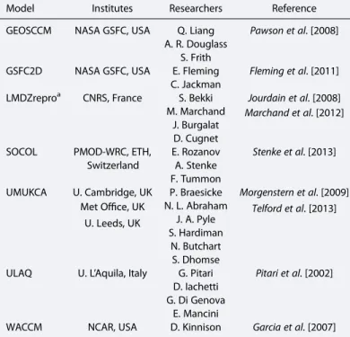
In this paper we discuss the model runs performed for SPARC [2013]. We present lifetime estimates of 11 long-lived SR ODSs from six three-dimensional (3-D) Chemistry-Climate Models (CCMs) and one 2-D model from groups worldwide for present-day and 2100 conditions (Table 1). The CCMs (or earlier versions thereof) par-ticipated in the Chemistry-Climate Model Validation Activity (CCMVal) for the WCRP’s SPARC Project [Eyring et al., 2005], and so the key processes which impact lifetimes (e.g., photolysis and stratospheric circulation) have already been evaluated extensively [e.g., Waugh and Eyring, 2008; SPARC CCMVal, 2010; Morgenstern et al., 2010; Butchart et al., 2011; Strahan et al., 2011].
CCMs participating in recent stratospheric ozone assessment efforts [e.g., WMO, 2011] used prescribed time-dependent mixing ratio boundary conditions (MBCs) at the surface to simulate the evolution of ODSs and GHGs in the atmosphere. This approach can lead to inconsistencies between the burden of the trace gas and CCM transport and loss if these rates differ from the real atmosphere for studies using past observations or to those in the model which created a future surface trace gas mixing ratio scenario. We investigate that consistency here by using CCMs to investigate differences that arise from using emissions, formulated asflux boundary condi-tions (FBCs), to specify the input of ODSs and GHGs.
The aim of this paper is to complement the updated lifetime estimates for SR species presented in SPARC [2013], which are partly based on CCM simulations, by providing further analysis of the models. In particular, we investigate the causes of model-model differences and variations in lifetime estimates within the same model. We also investigate how lifetimes may change in a future atmosphere. Section 2 describes how the
Table 1. List of CCMs and 2-D Model Used in This Study
Model Institutes Researchers Reference GEOSCCM NASA GSFC, USA Q. Liang Pawson et al. [2008]
A. R. Douglass S. Frith
GSFC2D NASA GSFC, USA E. Fleming Fleming et al. [2011] C. Jackman
LMDZreproa CNRS, France S. Bekki Jourdain et al. [2008] M. Marchand
J. Burgalat
Marchand et al. [2012] D. Cugnet
SOCOL PMOD-WRC, ETH, Switzerland
E. Rozanov Stenke et al. [2013] A. Stenke
F. Tummon
UMUKCA U. Cambridge, UK P. Braesicke Morgenstern et al. [2009] N. L. Abraham Met Office, UK J. A. Pyle S. Hardiman Telford et al. [2013] U. Leeds, UK N. Butchart S. Dhomse
ULAQ U. L’Aquila, Italy G. Pitari Pitari et al. [2002] D. Iachetti
G. Di Genova E. Mancini
WACCM NCAR, USA D. Kinnison Garcia et al. [2007] a
The LMDZrepro version used here has only 39 vertical levels, the same as in the CMIP5 LMDZ climate model [Dufresne et al., 2013], instead of 50 levels as in SPARC [2010].
lifetime simulations were formulated. The main results of model evaluation and lifetime estimation are contained in section 3. Our results are summarized in section 4. This paper does not attempt to suggest recommended lifetimes. For that the reader is referred to SPARC [2013] which provides best estimates based on results of our model runs combined with independent values from observations.
2. Model Experiments
We have used results from seven atmospheric models which performed simulations for the recent past, present, and future atmosphere. The model experiments are described in this section, along with our methods for deriving lifetimes.
2.1. Participating Models
We use simulations from six 3-D CCMs and one 2-D model, Goddard Space Flight Center (GSFC2D) (Table 1). All of these simulations used the same kinetic and photochemical recommendations from Jet Propulsion Laboratory (JPL) 10–6 [Sander et al., 2011] and were driven with the same surface boundary conditions for GHGs and ODSs, sea ice, and sea surface temperatures (including GSFC2D which was driven by the zonal mean surface tempera-tures from Goddard Earth Observing System Chemistry-Climate Model (GEOSCCM)). However, the models differ in dynamical schemes, e.g., advection, convection, cloud parameterization, and the inclusion or treatment of various atmospheric processes, e.g., solar cycle, quasi-biennial oscillation (QBO). The six 3-D CCMs all participated in SPARC CCMVal-2 and the report from that activity, SPARC CCMVal [2010], contains descriptions of the models and a detailed process-based evaluation. Updates to the models for the versions used here are described in SPARC [2013]. In this paper we focus on variations in lifetime estimates due to differences in model dynamics and transport.
2.2. Lifetime Experiments
We use a number of model simulations and types of tracers to investigate the relationships between surface fluxes, atmospheric burden, removal rates, and lifetime.
2.2.1. Model Simulations
We conducted and analyzed the following integrations: One transient simulation from 1960 to 2010 (TRANS) and two time slice simulations with 2000 conditions (TS2000) and 2100 conditions (TS2100) to calculate present-day and future lifetimes, respectively. Simulations TRANS and TS2000 allow us to compare lifetimes calculated in a full transient experiment with a steady state experiment. All models used the same mixing ratio boundary conditions for long-lived GHGs from the Coupled Model Intercomparison Project (CMIP) Representative Concentration Pathways (RCP) Scenario 4.5 (“historic” scenario before 2000), ODSs according to WMO [2011], and HFCs based primarily on Velders et al. [2009]. Sea surface temperatures and sea ice concentrations in all six 3-D CCMs are prescribed as monthly mean boundary conditions following the global sea ice concentration and sea surface temperature (HadISST1) data set provided by the UK Met Office Hadley Centre [Rayner et al., 2003]. We present here a brief description of the model simulations; for more detailed information, see SPARC [2013]. TRANS is a 50 year transient run from 1960 to 2010, based on the definition of the REF-B1 simulation used in CCMVal-2 [SPARC CCMVal, 2010, chapter 2; Morgenstern et al., 2010]. Note that while REF-B1 was a transient simulation with mostly stratosphere-only chemistry schemes, the TRANS simulations from four (SOCOL, ULAQ, WACCM (Whole Atmosphere Community Climate Model), and UMUKCA) of the six 3-D CCMs were run with stratosphere-troposphere coupled chemistry. All forcings in this simulation are taken from observations and are mostly identical to those described by Eyring et al. [2006] and Morgenstern et al. [2010] for REF-B1. This transient simulation includes all anthropogenic and natural forcings based on changes in trace gases, solar variability, volcanic eruptions, quasi-biennial oscillation (QBO), and sea surface temperatures/sea ice con-centrations (SSTs/SICs). Models that do not include a detailed tropospheric chemistry scheme (GEOSCCM, GSFC2D, LMDZrepro) prescribed their tropospheric OH values from the 3-D monthlyfields of Spivakovsky et al. [2000]. For models that have coupled stratosphere-troposphere chemistry schemes, emissions of ozone and aerosol precursors are from the RCP 4.5 scenario [Lamarque et al., 2011].
TS2000 is a 30 year time slice simulation for 2000 conditions, designed to diagnose steady state lifetimes and to facilitate the comparison of model output against constituent observations from various measurement data sets [SPARC, 2013]. This simulation is conducted with prescribed GHG, ODS, and HFC surface boundary conditions for 2000, but individual models were run with either repeating or interannually varying solar variability, volcanic eruptions, QBO, and SSTs/SICs for 2000 conditions. Thefinal 20 years are used for analysis.
TS2100 is similar to TS2000 but for assumed 2100 conditions and used to diagnose steady state lifetimes in a future climate with a recovered stratospheric ozone layer and a possibly different Brewer-Dobson circulation. This simulation was conducted with prescribed GHG (RCP 4.5 scenario) and ODS surface boundary conditions for 2100, but individual models were run with either repeating or interannually varying solar variability, QBO, and SSTs/SICs for 2100 conditions.
2.2.2. Additional ODS Tracers
Two additional sets of ODS tracers were embedded in the CCM simulations but uncoupled from the full chemistry scheme. One set of tracers used realistic surface emission FBCs (FBC), while the other used time-independent MBCs (CONST). Although the FBC and CONST tracers are driven with different boundary conditions, they are destroyed in the atmosphere with the same kinetics as the corresponding full chemistry MBC tracers. Note that potential differences in simulated FBC concentrations do not affect the modeled chemistry and physics as these tracers are uncoupled from the interactive chemistry scheme which is based on the MBC tracers.
2.2.2.1. FBC Tracers
We include two stratospheric removal FBC tracers in the CCM simulations for CFC-11 (CFC-11_FBC) and CFC-12 (CFC-12_FBC), the two most abundant chlorinated ODSs that have ready-to-use bottom-up emission estimates. These two FBC tracers are initialized with similar conditions to the MBC tracers at the start of the simulation and evolve with geographically resolved surface emissionfluxes and atmospheric losses via photolysis and reaction with O(1D). The model runs also included two tropospheric removal (TR) FBC tracers for CH3CCl3and
HCFC-22 which are discussed in SPARC [2013].
2.2.2.2. CONST Tracers
Three constant tracers are embedded in the simulations: CFC-11_CONST, CFC-12_CONST, and N2O_CONST.
These tracers are lost with the same kinetics as the MBC tracers but have a prescribed constant 100 parts per trillion by volume (pptv) surface boundary condition.
We use the combination of MBC, FBC, and CONST tracers from the same model runs to examine how surface emission trends, atmospheric abundance, and trace gas distribution impact atmospheric lifetime.
2.3. Methods for Estimating Lifetimes
The atmospheric lifetime (τ) is generally defined as the ratio of atmospheric burden to the removal rate of the species. Therefore, the lifetime of a species depends not only on the properties of the molecule (e.g., ab-sorption cross section) but also on its emission history and the atmospheric state. There is no unique value for a lifetime of a species and various definitions exist. An instantaneous lifetime is defined at a fixed moment in time (or over a short time window) and is estimated from the atmospheric state at that time. In general lifetimes based on observations are instantaneous ones valid at the time of the observations. A steady state lifetime (τss) is the lifetime when the species is at steady state in the atmosphere (i.e., sources = sinks). This
rarely occurs in the real atmosphere for long-lived source gases, but steady state conditions can easily be set up in a model simulation (e.g., in a time slice run). Note that measurements of instantaneous lifetimes can be corrected in order to report observational estimates ofτss. Partial lifetimes can also be defined. These can be
the lifetime of a species against loss by a particular process (e.g.,τphotfor loss by photolysis,τO1Dfor loss by
reaction with O(1D),τOHfor loss by reaction with OH), or the loss of a species within a subregion of the
atmosphere (e.g.,τstratfor loss within the stratosphere andτtropfor loss within the troposphere). The overall
lifetime can be calculated from its components by 1 τtotal¼ 1 τ1þ 1 τ2þ … (1)
The atmospheric partial lifetime,τatmos, of a trace gas is calculated in a model using the globally integrated
sum of its mass-weighted atmospheric loss rate at all locations. Note that except for species that have surface losses, e.g., CCl4among those considered here, the atmospheric partial lifetimeτatmosis equivalent to the
global atmospheric lifetimeτ. In this paper all of our quoted lifetimes are atmospheric lifetimes.
Aside from uncertainty associated with kinetic rates [see SPARC, 2013], uncertainty in lifetime estimates can also arise from variations in the representation of model transport and chemical processes. For species that are removed mainly by UV photolysis with maximum loss in the stratosphere, lifetimes depend not only on
the photolysis rate but are also affected by how fast the atmospheric circulation moves air through the maximum loss region.
Because lifetime depends on burden, a potentially important and easily avoided source of model error (and model-model differences) relates to the treatment of surface orography. For SR tracers the model burden is dominated by the troposphere where the tracer is inert and well mixed. In the extreme case, if a model ignored surface orography and assumed a uniform surface pressure of 1013 hPa, it would have an atmospheric mass below 400 hPa about 5% larger than a model with realistic topography and a global mean surface pressure of around 985 hPa. For such models (here GSFC2D and ULAQ) we can account for this by assuming a constant atmospheric mixing ratio from 400 hPa to the surface at 1013 hPa and applying a mass correction factor of 0.95 to the calculated burden below 400 hPa. For the FBC tracers this issue would manifest itself in a different way. Models will have the same emitted tracer mass but in a model which ignores surface orography this mass will be distributed over a deeper atmosphere, likely leading to smaller tropospheric mixing ratios. This could lead to a smaller concentrationflux through the tropopause into the stratospheric sink region and therefore a longer lifetime estimate. However, this small potential effect is not easy to treat using archived data and so is ignored here. This results in a slight difference in calculated lifetimes between MBC tracers and their corresponding FBC tracers.
3. Results
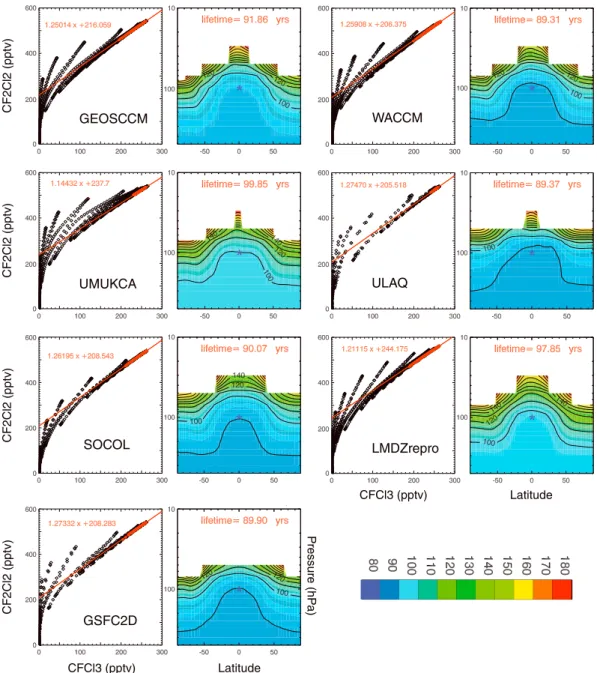
To illustrate the importance of chemical loss in different regions, Figure 1 shows the annually averaged zonal mean loss rates of four ODSs. CFC-11, CFC-12, and N2O are SR species with chemical loss occurring
solely in the stratosphere. The shortest lived of these, (CFC-11), is destroyed lower in the stratosphere compared to longer-lived CFC-12 and N2O. Although CBrClF2(Halon-1211) is also primarily destroyed via
photolysis, the majority of its loss occurs in the troposphere as it can be removed by photolysis at UV wavelengths up to 320 nm. For all species considered here, about 75–95% of the atmospheric removal occurs between 60°N and 60°S with>50% of the loss occurring in the tropics (within 30° of the equator). Therefore, the performance of the models in the tropical region is a key to calculating accurate lifetimes [see SPARC, 2013]. In particular, the ability of the models to simulate realistic stratospheric tracer transport in the tropics is critical and this is investigated in detail in section 3.1. Section 3.2 discusses issues related to the quantification of lifetimes from the model runs for present-day conditions. Section 3.3 discusses how lifetimes may change in a future climate.
3.1. Model Mean Age and Comparison With Observations
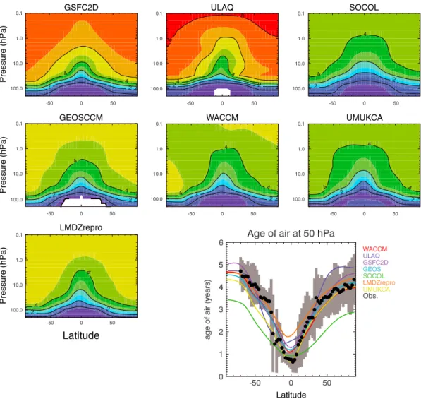
Age-of-air is a simple but very useful diagnostic for testing the stratospheric circulation in CCMs and is discussed in detail in SPARC CCMVal [2010]. Figures 2 and 3 show the stratospheric modeled age-of-air from the CCM runs for present-day conditions and comparison with values derived from balloon and aircraft observations [Andrews et al., 2001; Engel et al., 2009]. For the analysis here the modeled age was set to zero at the tropical tropopause because the tracers used to diagnose age in these runs were initialized in the lower troposphere and therefore include the transit time to the tropopause. This procedure had the largest impact on UMUKCA which otherwise produced a tropopause age with a value of around 0.5 years; the shift of Figure 1. Latitude-pressure cross sections of zonally integrated annual loss rates of Halon-1211, CFCl3, CF2Cl2, and N2O between 2000 and 2005 from the WACCM TRANS simulation with warm colors indicating faster loss rates. The solid contours outline the regions within which 95%, 75%, and 50% of the loss occurs.
reference for the other models was smaller than this. This may be partly due to UMUKCA using an altitude-based vertical coordinate compared to the rest of the models which use pressure-altitude-based coordinates. The diagnostics were performed on common monthly mean pressurefields which would have resulted in larger interpolation of the UMUKCAfields. In the lower stratosphere (50 hPa) the CCMs tend to agree well with each other and with the observed variation in age from the tropics to the poles. One exception is SOCOL, which produces mean age-of-air about 1 year younger than the observations at high latitudes. Sensitivity tests with a version of SOCOL with higher vertical resolution (90 levels instead of 39) showed that the stratospheric circulation is slower and the age-of-air latitudinal gradient increases (not shown), indicating that the young age of air in Figure 2 is due at least in part to the coarse-model vertical resolution. LMDZrepro also stands out as having air in the lower stratosphere (LS) much older than the other models, although the agreement is better higher up and the model produces relatively short lifetimes (see further discussion in section 3.2.4). The LMDZrepro version used here has only 39 vertical levels, the same levels as in the CMIP5 Laboratoire de Météorologie Dynamique (LMDZ) climate model [Dufresne et al., 2013], whereas the version used in SPARC [2010] had 50 levels. The 50-level version did not show this strong bias in the LS mean age-of-air [SPARC, 2010]. Clearly, the reduction in the vertical resolution in the stratosphere has a large negative impact on the quality of the simulated stratospheric circulation. Overall, the models show a large variation in age in the middle and upper stratosphere. At around 50 km SOCOL, WACCM, LMDZrepro, GEOSCCM, and UMUKCA
Latitude GSFC2D GEOSCCM UMUKCA Pressure (hPa) Pressure (hPa) Pressure (hPa) Latitude LMDZrepro ULAQ SOCOL WACCM
Figure 2. Mean age-of-air (years) calculated from the last 15 years of the TS2000 runs. Contour interval 0.5 year. (bottom, right) The modeled mean age at 50 hPa with derived age-of-air from ER-2 aircraft measurements [Andrews et al., 2001] along with their 2σ uncertainty shown as grey shading.
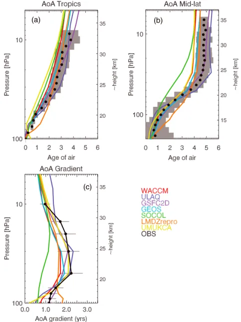
produce ages that are 1–2 years younger than ULAQ and GSFC2D. The balloon observations used in Figure 3 only provide data up to ~30 km but tend to show the models with the older ages are more realistic. Figure 3 also shows the gradient in mean age between the northern midlatitudes and the tropics. This diag-nostic evaluates the tropical ascent rate [Neu and Plumb, 1999; CCMVal SPARC, 2010]. GSFC2D, ULAQ, and UMUKCA show the best agreement with the observations in the 18–27 km (~70–20 hPa) region where CFC-11 experiences significant loss. GEOSCCM and WACCM have gradients that indicate their tropical ascent is some-what faster but still within the uncertainty range of the observations over most of this range. SOCOL is the only model showing significantly fast ascent throughout the tropical lower and middle stratosphere. LMDZrepro has mixed results, with very slow ascent below 19 km but fast ascent above. Overall, these results show that ULAQ, GEOSCCM, GSFC2D, UMUKCA, and WACCM have reasonable tropical ascent rates. Horizontal mixing (i.e., recirculation) into the tropics, which impacts tropical mean age and the ODS burden in the maximum loss region,
(a) (b)
(c)
Figure 3. Mean age-of-air from present-day CCM simulations for (a) tropics (10°N–10°S) and (b) northern midlatitudes (35°N–45°N). Note the different altitude ranges for Figure 3b. The ages are 15 year averages of the model zonal mean output from TS2000 runs. Figures 3a and 3b also show estimates derived from observations [Andrews et al., 2001; Engel et al., 2009] as used in Strahan et al. [2011], with their 1σ uncertainty shown as grey shading. (c) The mean age gradient between the northern midlatitudes and tropics from the model runs versus observations with their 1σ uncertainties [see SPARC CCMVal, 2010, Figure 5.5].
is not assessed by this diagnostic. SPARC [2013] has further comparison of the model runs with obser-vations of some of the target SR species.
3.2. Model Lifetime Calculations 3.2.1. Evolution of Lifetimes From 1960s to Present
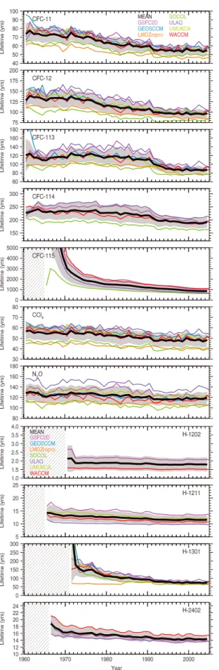
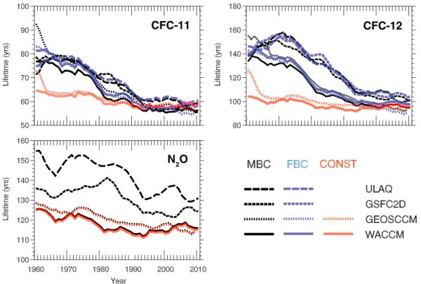
The time evolutions of the instantaneous lifetimes (τtransient) of all SR species and halons from the
TRANS run are shown in Figure 4. Note that while the TRANS run extends from 1960 to 2010, only the results between 1960 and 2006 are shown as that is the period for which all model results were available. Theτtransientdisplays significant
interannual variations with year-to-year 1σ vari-ance of ±3–5%. Overall, the model calculations clearly show a decrease in lifetime for all SR spe-cies due to the diminishing imbalance between surfacefluxes and atmospheric losses as the atmosphere approaches steady state conditions [Martinerie et al., 2009]. The contrast in lifetime between CFC MBC and CONST tracers, shown in Figure 5, clearly demonstrates that the main cause of the decrease in CFC-11 and CFC-12 lifetimes can be attributed to trends in their atmospheric concentrations. Secondary causes of the decrease in lifetime of the SR species are likely due to the combination of higher-altitude O3depletion that
increases photolytic destruction and any changes in the Brewer-Dobson circulation [Fleming et al., 2011]. The CONST tracers implemented in the GEOSCCM and WACCM models suggest that the changes in photolysis and circulation together explain a decrease of ~5 years (~8% with respect to the ~57–58 years in 2000s) in CFC-11 lifetime and ~7 years (~7% with respect to the ~93–96 years in 2000s) in CFC-12 lifetime between the 1960s and 2000s. Changes in atmospheric concentrations lead to a decrease of ~15 years in CFC-11 lifetime and ~30 years in CFC-12 lifetime over the same period. The small difference between the lifetimes of N2O
and its CONST tracer implies that the lifetime of N2O is not affected by the relative small change in
its atmospheric concentration. The ~7 year decrease in N2O lifetime from 1960s to 2000s (6% with respect
to a 115 year lifetime in 2000s) is mainly due to changes in photolysis and atmospheric circulation.
Figure 4. Time evolution of modeled instantaneous atmospheric lifetimes (τtransient, years) of SR species between 1960 and 2006 from the TRANS simulations. Model mean lifetimes (thick black lines) and 1σ variance (grey shadings) are also shown. The grey-hatched area indicates where atmospheric concentrations of the corresponding ODSs are close to zero.
Figure 6 compares model hemispheric mean FBC tracers with observations. The MBC tracers are forced to have a tropospheric mixing ratio which matches the observations, while for the FBC tracers this is a predicted quantity. Given realistic emission data, the comparison of the FBC tracers with observations, therefore, tests the models’ ability to reproduce observed loadings through realistic lifetimes and shows the degree of model-model variability which would occur if the simulations used FBCs. The FBC tracers display significant interhemispheric and seasonal variations. The lifetimes for the FBC tracers are similar to those for the MBC tracers (see Table 4 below) because the sink will scale as the atmospheric burden changes so that the lifetime just depends on the model transport and chemistry. As the models generally perform well in reproducing the observed surface mixing ratios, this shows that their transport and chemical loss rates are reasonable. However, despite its relatively long FBC lifetimes, ULAQ simulates a low burden of CFC-11 and CFC-12 with time which carries on increasing when other models have turned over. Further comparison of the 2000 steady state and instantaneous lifetimes of MBC, FBC, and CONST tracers is shown in SPARC [2013]. Note that the instantaneous lifetimes in 2000 for the listed ODSs are not statistically different from their year 2000 steady state lifetimes, despite their different trends in atmospheric concentrations (decreasing trends for CFC-11, CFC-12, CCl4, and increasing trends for N2O).
3.2.2. Present-Day Steady State Lifetimes
Table 2 lists the steady state ODS lifetime for 2000 conditions from the seven models. The models agree fairly well in lifetime estimates for many SR species, with calculated lifetimes in general within 10% of the multimodel mean. Lifetimes of several major SR species, e.g., CCl4, CFC-11, CFC-12, N2O, from the SOCOL and
LMDZrepro models are shorter than the other models, most likely due to the fast tropical ascent in the lower stratosphere (see sections 3.1 and 3.2.4).
Table 3 summarizes the present-day multimodel mean steady stateτssand 1σ variance of the 11 ODSs,
along with thefinal recommendations from SPARC [2013]. The model mean lifetimes and their variances (note that these are not uncertainty estimates) are calculated from the inverse of the mean and the variance of all available modeled loss rates. Table 3 also lists partial lifetimes in the stratosphere and troposphere and partial lifetimes associated with different loss processes, i.e., photolysis and reaction with
CFC-11
CFC-12
N
2O
Figure 5. Time evolution of modeled atmospheric lifetimes of MBC CFC-11, CFC-12, and N2O (black lines) between 1960 and 2010 from the TRANS simulations and their corresponding FBC (blue lines) and CONST (red lines) tracers when available. For clarity, the lifetimes are smoothed with a 5 year running meanfilter.
O(1D). Table 4 compares the lifetimes diagnosed from different types of model tracer. The model mean lifetime esti-mates for CFC-11, CCl4, and all four
halons are significantly different from the WMO [2011] values. Photolytic destruction is the dominant loss process for all SR species with reaction with O(1D)
as a minor loss channel for CFCs and N2O. Reaction with O(
1
D) is particularly important for CFC-114 and CFC-115, accounting for 27% and 38% of their global loss, respectively. Although photolysis is the predominant removal process for Halons, for three (H-1202, H-1211, >and H-2402) of the four studied, the majority of the removal occurs in the troposphere. (Partial lifetimes with respect to different chemical loss pro-cesses for all SR species are detailed in SPARC [2013, chapter 3]). We note that updates to kinetic and photochemical parameters in SPARC [2013], which are not used here, resulted in significant changes in the lifetimes of some of the SR species, especially CFC-115, Halon-1202, Halon-1211, and Halon-2402. These large differences between the SPARCfinal recommendations and our model mean lifetimes for these species are mainly due to the differences between the recommended reaction rates for CFC-115 + O(1D) and, for the halons, the UV absorption cross sections. The SPARC recommended rates are based on new laboratory measurements documented in Baasandorj et al. [2013] and Papanastasiou et al. [2013].
3.2.3. Relative Lifetimes From Tracer-Tracer Correlations
For SR species under steady state conditions tracer-tracer correlations can be used to derive relative lifetimes. As explained by Plumb and Ko [1992], two tracers with lifetimes longer than quasi-horizontal mixing time scales should be in“slope equilibrium” and produce a compact correlation. Species with lifetimes longer than vertical transport time scales will also be in“gradient equilibrium” and the compact correlation will be linear. Figure 6. Time evolution of global mean surface concentration (pptv) of
(top) CFC-11 and (bottom) CFC-12 from observations and the modeled FBC tracers in the TRANS simulations from 1960 to 2010. The observations are from stations averaged over the Northern and Southern Hemispheres. The model results are also shown averaged over the Northern (solid lines) and Southern (dotted lines) Hemispheres.
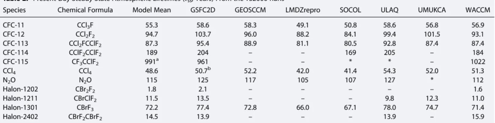
Table 2. Present-Day Steady State Atmospheric Lifetimes (τss, Years) From the TS2000 Runs
Species Chemical Formula Model Mean GSFC2D GEOSCCM LMDZrepro SOCOL ULAQ UMUKCA WACCM
CFC-11 CCl3F 55.3 58.6 58.3 49.1 50.8 58.6 56.8 56.9 CFC-12 CCl2F2 94.7 103.7 96.0 88.2 84.1 99.4 101.5 93.1 CFC-113 CCl2FCClF2 87.3 95.4 88.9 81.1 80.5 92.8 87.4 87.4 CFC-114 CClF2CClF2 189 204 – – 169 205 – 184 CFC-115 CF3CClF2 991a 961 – – * * – 1022 CCl4 CCl4 48.6 50.7b 52.2 42.0 41.4 54.3 52.0 51.3 N2O N2O 115 125 117 105 107 127 * 112 Halon-1202 CBr2F2 1.8 2.1 – – – – – 1.6 Halon-1211 CBrClF2 11.5 13.5 – – – 9.8 12.3 11.0 Halon-1301 CBrF3 72.2 77.4 72.8 66.0 67.1 78.0 74.7 71.4 Halon-2402 CBrF2CBrF2 14.5 13.9 – – – 13.9 – 15.9 a
We calculate the mean lifetime of CFC-115 as the average of the GSFC2D and WACCM lifetimes as SOCOL and ULAQ specified a too large reaction rate constant for O(1D) and CFC-115 in their calculations.
b
For SR species the slope of tracer-tracer correlation plot for points below the photochemical loss region (i.e., tropical lower stratosphere) can be approximated by the ratio of the tracer lifetimes:
τ2 τ1¼ q2 q1 dq1 dq2 (2)
where q1and q2are volume mixing ratios. Plumb [1996] refined this “global mixing” model to account for
sub-tropical barriers to transport.
Equation (2) has been applied to derive estimates of relative lifetimes from observations [e.g., Volk et al., 1997; Brown et al., 2013; Laube et al., 2013]. In these studies the slope of the tracer-tracer correlation is only eval-uated in the extratropics to avoid errors related to subtropical transport barriers. Moreover, time trends in the tropospheric mixing ratios of the source gases complicate the analysis as the atmosphere will not be in steady state. The application of equation (2) to model experiments is more straightforward as we can perform idealized steady state experiments with constant source gas surface boundary conditions.
We have derived relative lifetimes from simulation TS2000 by correlating model tracers with respect to CFC-11 using the last 15 years of the run when the steady state assumption should be valid (see Figure 7). To evaluate the lifetime using equation (2) mean tracer values at/below 100 hPa in the extratropics (35°–60° latitude) were Table 3. Present-Day Multimodel Mean Steady State Atmospheric Lifetimes (τss, Years) Compared to Results From WMO [2011] and SPARC [2013]a
Species WMO [2011] SPARC [2013]
Model Mean Model Variance
τstrat τtrop τphot τO1D
τss % (Years) CFC-11 45 52 55.3 (7) 8% (4.2) 57.0 1870 56.4 2930 CFC-12 100 102 94.7 (7) 8% (7.3) 95.5 11600 100 1750 CFC-113 85 93 87.3 (7) 6% (5.5) 88.4 7620 92.9 1460 CFC-114 190 189 189 (4) 10% (18.0) 191 19600 261 684 CFC-115 1020 540 991c(2) 4% (43.1) 997 126000 1590 2610 CCl4b 35 44 48.6 (7) 12% (5.6) 50.6 1230 48.7 --N2O 114d 123 115 (6) 8% (9.0) 116 15600 127 1180 Halon-1202 2.9 2.5 1.8c(2) 21% (0.4) 15.3 2.0 1.8 10600 Halon-1211 16 16 11.5c(4) 14% (1.6) 33.5 17.3 11.5 8040 Halon-1301 65 72 72.2 (7) 7% (4.7) 73.5 4490 73.3 5260 Halon-2402 20 28 14.5c(3) 8% (1.1) 33.8 25.1 14.4 6790 a
The SPARC [2013] lifetimes are partly based on our model runs but also include estimates from observations where possible. Also shown are the partial lifetime contributions to the modelτss. Species whose WMO [2011] lifetimes are less (or more) than model mean– (+) 1σ variance are highlighted in bold. The number of models which contribute to the mean are shown in parentheses in column 4 (see Table 2).
b
The CCl4lifetime from the models isτatmos, compared withτtotalfrom WMO [2011] which accounts for ocean and soil losses. c
Based on JPL-2010 [Sander et al., 2011]. Significantly different lifetimes are obtained using kinetic and photochemical parameters updated for SPARC [2013, chapter 3].
d
Lifetime from Intergovernmental Panel on Climate Change (IPCC) [2007].
Table 4. Comparison of Model Steady State Lifetime (τss, Years) From the TS2000 Simulation With the Transient Lifetime
(τTransient) for MBC Species and Their FBC and CONST Tracers in Year 2000 From the TRANS Simulation
Species GSFC2D GEOSCCM LMDZrepro SOCOL ULAQ UMUKCA WACCM CFC-11 τSS 58.6 58.3 49.1 50.8 58.6 56.8 56.9 τtransient, MBC 56.6 60.0 47.0 49.5 58.2 56.3 55.1 τtransient, FBC 60.0 58.7 – – 60.6 61.4 55.2 τtransient, CONST – 60.4 – – – – 57.1 CFC-12 τSS 103.7 96.0 88.2 84.1 99.4 101.5 93.1 τtransient, MBC 102.1 98.5 85.0 80.5 101.4 99.9 93.3 τtransient, FBC 99.1 96.1 – – 105.0 109.7 93.0 τtransient, CONST – 97.5 – – – – 92.1 CCl4 τSS 50.7 52.2 42.0 41.4 54.3 52.0 51.3 τtransient, MBC 49.2 53.5 40.0 41.0 53.8 51.2 50.1 N2O τSS 125 117 105 107 127 – 112 τtransient, MBC 124 120 – 105 130 – 113 τtransient, CONST – 119 – – – – 112
used. Table 5 shows the derived relative stratospheric lifetimes, along with the corresponding absolute lifetime assuming aτCFCl3of 55 years, which is close to the multimodel mean in Table 2.
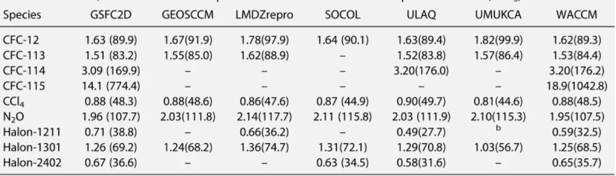
The relative lifetimes shown in Table 5 show a generally good level of agreement between the models. For example, the relative lifetime of CFC-12 varies from 89.3 years in WACCM to 99.9 years in UMUKCA. This range is much narrower than the range of absolute lifetimes of 84.1 to 103.7 given in Table 2. This is also the case for CFC-113 (83.2–88.9 years versus 80.5–95.4 years), CCl4(44.6–49.7 years versus 41.4–54.3 years), and N2O
(107.5–117.7 years versus 105–127 years). For Halon-1301 UMUKCA produces a very curved correlation which
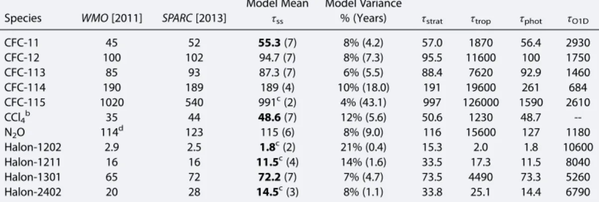
GEOSCCM WACCM UMUKCA ULAQ SOCOL LMDZrepro GSFC2D CFCl3 (pptv) CFCl3 (pptv) Latitude Latitude CF2Cl2 (ppt v) CF2Cl2 (ppt v ) CF2Cl2 (ppt v ) CF2Cl2 (ppt v) P ressur e (hP a )
Figure 7. Plots showing the calculation of relative lifetime for CFC-12 from tracer-tracer correlation plots for the seven models. Results are shown for average of last 15 years of the TS2000 runs. (columns 1 and 3) The CFC-12 (CF2Cl2) versus CFC-11 (CFCl3) correlation plots. The points in orange arefitted to a straight line (equation on top left). For all models except UMUKCA the orange points were selected as those between 35°S–60°S and 35°N–60°N, below 100 hPa and within 30% of the maximum tracer values in this region. For UMUKCA the orange points were furtherfiltered to use those with the minimum value of CFC-12 for any value of CFC-11. (columns 2 and 4) The relative lifetime of CFC-12 evaluated using equation (2) (see text) and an assumed CFC-11 lifetime of 55 years. The lifetime at 100 hPa in the tropics (location of blue star) is shown in Figure 7 (columns 2 and 4) and used in Table 5.
is hard tofit with an objective straight line. Aside from its low relative lifetime of 56.7 years, for the other models the relative lifetimes in Table 5 also show less spread than Table 2 for Halon-1301 (68.2–74.7 years versus 66.0–78.0 years). Also, while LMDZrepro, for example, generally produces low absolute lifetimes in Table 2, this is not the case for the relative lifetimes. Problems with the representation of ascent and mixing in a model affect the lifetime of both species similarly. Thus, the calculation of a relative lifetime reduces the impact of transport issues, with the result that relative lifetimes depend more strongly on chemical loss processes. This explains why there is better agreement among the model lifetimes in Table 5. Halons 1211 and 2402 have significant tro-pospheric loss; the tracer-tracer correlation method will diagnose stratospheric lifetimes (compare to Table 3). The tracer-tracer correlations for UMUKCA in the lower stratosphere, based on the monthly mean output were not as compact as the other models and needed to befitted in a more selective way (see Figure 7 caption). Note again that UMUKCA is unique among the models presented here in using a hybrid height coordinate and a nonhydrostatic dynamical core. This noncompactness in the tracer-tracer correlations may also be due to the semi-Lagrangian advection scheme and the associated tracer massfixer used in UMUKCA. The impact of this scheme on advected tracers is discussed by Morgenstern et al. [2009].
3.2.4. Variation of Lifetimes With Modeled Age-of-Air
The lifetime of a SR tracer depends on stratospheric transport, i.e., the Brewer-Dobson circulation. In section 3.1 we examined simulated tropical and midlatitude mean profiles and evaluated model tropical ascent rate with rates derived from observations. In this section we explore the relationship between the derived lifetimes and age-of-air for individual models.
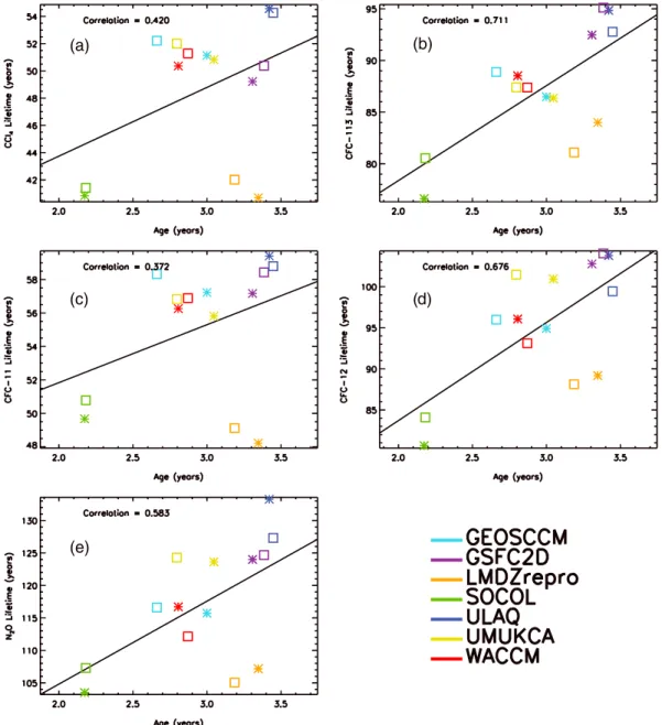
Figure 8 shows correlation plots of derived lifetimes with the global mass-weighted average of stratospheric mean age-of-air (70–1 hPa) for selected SR species. For this analysis the mean age-of-air for each model has been reset to zero at the tropical tropopause (see section 3.1). Overall, there is a positive correlation: Models with older mean age-of-air give longer lifetimes. LMDZrepro tends to be an outlier because its mean age below 20 km is too high (Figure 3). For the other models a good straight-line correlation is obtained whether the mean age-of-air is averaged from 100 hPa (not shown) or 70 hPa. However, the mass-weighting means that the large age-of-air values in LMDZrepro in the lower stratosphere, in a region where SR species are not strongly photolyzed, will strongly bias the results. Overall, the good correlation between the modeled life-times and mean age-of-air supports the results of relative lifelife-times discussed in section 3.2.3 and highlights the influence of transport on the modeled lifetimes of SR species.
Figure 9 shows the correlation between modeled lifetimes and the difference in mean age between two levels in the tropical lower stratosphere for CFC-11 and CFC-12. The chosen altitudes span the main loss region for each species. (Although the CFC-12 maximum loss region extends to ~5 hPa, we are limited to a maximum altitude of 32 km (10 hPa) for tropical mean age observations). This quantity is related to the time taken for air to ascend through this loss region. Mean age changes in the tropical profile result from vertical advection and mixing between the tropics and midlatitudes (i.e., recirculation into the ascending air). The stronger correlation seen in Figure 9 than in Figure 8 suggests that lifetimes are particularly sensitive to the combined effects of ascent and mixing in the tropical lower midstratosphere. Figures 9a and 9b (solid vertical line) represent the observed mean age gradient, with uncertainties shown by the dashed vertical lines. Tropical mean age differences from 70 to 20 hPa for the transient experiment for GEOSCCM, UMUKCA, WACCM,
Table 5. Relative Steady State Stratospheric Lifetimes (τstrat) for Year 2000 Conditions for SR Species From the TS2000 Model Simulations, Derived From Extratropical Tracer-Tracer Correlations Compared to CFC-11 (CFCl3)a
Species GSFC2D GEOSCCM LMDZrepro SOCOL ULAQ UMUKCA WACCM CFC-12 1.63 (89.9) 1.67(91.9) 1.78(97.9) 1.64 (90.1) 1.63(89.4) 1.82(99.9) 1.62(89.3) CFC-113 1.51 (83.2) 1.55(85.0) 1.62(88.9) – 1.52(83.8) 1.57(86.4) 1.53(84.4) CFC-114 3.09 (169.9) – – – 3.20(176.0) – 3.20(176.2) CFC-115 14.1 (774.4) – – – – – 18.9(1042.8) CCl4 0.88 (48.3) 0.88(48.6) 0.86(47.6) 0.87 (44.9) 0.90(49.7) 0.81(44.6) 0.88(48.5) N2O 1.96 (107.7) 2.03(111.8) 2.14(117.7) 2.11 (115.8) 2.03 (111.9) 2.10(115.3) 1.95(107.5) Halon-1211 0.71 (38.8) – 0.66(36.2) – 0.49(27.7) b 0.59(32.5) Halon-1301 1.26 (69.2) 1.24(68.2) 1.36(74.7) 1.31(72.1) 1.29(70.8) 1.03(56.7) 1.25(68.5) Halon-2402 0.67 (36.6) – – 0.63 (34.5) 0.58(31.6) – 0.65(35.7) a
Values in parentheses are the corresponding lifetimes assumingτCFCl3= 55 years. b
and GSFC2D fall within the observational uncertainty. These four models have the most realistic tropical ascent over this range (Figure 3) and produce a very small range of CFC-11 lifetimes: 56.8–58.6 years from the TS2000 runs (Figure 9, squares; see Table 2). The most realistic transport over the 70–10 hPa range is seen in GEOSCCM, WACCM, and GSFC2D, with ULAQ and UMUKCA just outside the uncertainty range. The CFC-12 lifetimes calculated from thesefive TS2000 model runs span 93.1–103.7 years. The models with tropical ascent rates that are too fast (SOCOL and LMDZrepro) have the shortest lifetimes for CFC-11 (<51 years) and CFC-12 (<89 years) and have tropical mean age gradients that fall outside of the observed range. Given that the LMDZ lifetimes are lower than most other models in spite of relatively old air below 19 km (70 hPa), we conclude that fast ascent through the key loss region (i.e., above 70 hPa) is the primary factor influencing lifetimes.
3.3. Future Lifetimes Estimates
Atmospheric changes could modify tracer lifetimes in various ways in the future atmosphere. For example, a speedup in the Brewer-Dobson circulation in the critical region for stratospheric loss would be expected to
(a) (b) ) d ( (c) (e)
Figure 8. Correlation of modeled lifetimes (years) with the global mass-weighted average of stratospheric mean age-of-air from 70 hPa to 1 hPa (years) for (a) CCl4, (b) CFC-113, (c) CFC-11, (d) CFC-12, and (e) N2O. Mean results are shown from run TS2000 (squares) and years 2000–2009 from run TRANS (asterisks).
lead to a reduction in the lifetime of photo-lytically removed species [Butchart and Scaife, 2001]. Lin and Fu [2013] analyzed the Brewer-Dobson circulation changes in CCMVal-2 model experiments and found that while models consistently simulated an acceleration of both the shallow and deep branches of the Brewer-Dobson circulation (70–30 hPa and above 30 hPa), the acceler-ation of the deep branch was much smaller. They also noted significant differences between models.
Table 6 compares the lifetimes for TS2000 and TS2100 for six models that conducted both runs. The models predict different responses in future atmospheric lifetimes of SR species. GEOSCCM, SOCOL, and UMUKCA show a decrease in lifetimes in most of the SR species, while WACCM shows a slight increase in all SR species. The future lifetime changes predicted by GSFC2D and ULAQ are somewhat mixed, with increases for some and decreases for others. A comparison of change in mean age-of-air between the simulations for 2100 and 2000 suggests that all models, except WACCM, show a speeding up of the Brewer-Dobson circulation although the magnitude of this change varies (Figure 10). GEOSCCM, GSFC2D, and SOCOL show only a small decrease in mean age (~1–3 months), while UMUKCA and ULAQ show larger changes. WACCM shows a slight speedup (~0–1 month) of the shallow branch of the Brewer-Dobson circulation but a slowdown (~0–2 months) of the deep branch. However, such a weak change in
(a)
(b)
Figure 9. Correlation of modeled lifetimes (years) with the differ-ence in mean age-of-air between two levels in the tropics for (a) CFC-11 (age difference between 70 hPa and 20 hPa), and (b) CFC-12 (age difference between 70 hPa and 10 hPa). Results are shown from run TS2000 (square) and years 2000–2009 from run TRANS (asterisk). Also shown are estimates of the observed tropical mean age difference (vertical solid line) and its 1σ uncertainty (dashed vertical lines) using the data shown in Figure 3a interpolated to 10, 20, and 70 hPa.
Table 6. Steady State Atmospheric Lifetimes (τss, Years) for 2000 and 2100 Conditions From the TS2000 and TS2100 Simulations From Six Models
Species
Model Mean GSFC2D GEOSCCM SOCOL ULAQ UMUKCA WACCM
2000a 2100 2000 2100 2000 2100 2000 2100 2000 2100 2000 2100 2000 2100 CFC-11 56.5 55.2 58.6 57.7 58.3 54.7 50.8 49.3 58.6 57.6 56.8 55.2 56.9 57.7 CFC-12 95.8 95.3 103.7 103.5 96.0 90.6 84.1 81.9 99.4 104.2 101.5 98.8 93.1 96.7 CFC-113 88.5 87.8 95.4 94.4 88.9 83.4 80.5 79.1 92.8 96.6 87.4 85.5 87.4 90.6 CFC-114 189 193 204 206 – – 169 171 205 205 – – 184 192 CFC-115 991 1015 961 981 – – – – – – – – 1022 1052 CCl4 49.9 48.6 50.7 49.9 52.2 48.7 41.4 40.2 54.3 52.9 52.0 50.4 51.3 51.8 N2O 117 118 125 125 117 111 107 107 127 132 – – 112 118 H1202 1.8 2.0 2.1 2.5 – – – – – – – – 1.6 1.6 H1211 11.5 11.9 13.5 13.4 – – – – 9.8 10.0 12.3 13.5 11.0 11.4 H1301 73.4 73.1 77.4 76.8 72.8 68.6 67.1 66.1 78.0 79.2 74.7 76.2 71.4 73.5 H2402 14.5 14.8 13.9 14.0 – – – – 13.9 14.2 – – 15.9 16.4 a
circulation in WACCM might not be statistically significant. On the other hand, all models predict a decrease in photolysis (J) rates under 2100 conditions with the recovered ozone layer and a cooler stratosphere, though the relative changes in J rates vary between models and species. ULAQ and UMUKCA predict the strongest reduction in J rates, e.g., ~13% decrease in JCFC-11in the tropical lower stratosphere
between 10 and 100 hPa with respect to the 2000 conditions, while GSFC2D, WACCM, and GEOSCCM show a much weaker reduction of 5–6%. SOCOL displays a medium response of ~9% reduction in the corre-sponding JCFC-11rate. From a multimodel mean perspective, the decrease in lifetime due to a faster
Brewer-Dobson circulation cancels with the increase in lifetime due to weaker photolysis. Therefore, the modeled atmospheric lifetimes for SR species under 2100 conditions do not change significantly from the lifetimes under 2000 conditions.
It is important to note that the projections of ODS lifetime changes in a future climate depend upon the choice of the GHG scenario used to drive the TS2100 run. We used RCP 4.5 but higher levels of CH4, N2O, and CO2 from RCP 6.0 (the more likely scenario) or RCP 8.5 will lead to a different
response in atmospheric circulation and ozone concentration, therefore a different future lifetime for the targeted ODSs.
Figure 10. Difference in mean age-of-air (months) between CCM runs for 2100 and 2000. (Note: LMDZrepro did not perform TS2100 run.)
4. Conclusions
We have used results from seven global models (six 3-D CCMs and a 2-D model), integrated with the same standard photochemical data to estimate atmospheric lifetimes of source gases emitted at the surface and removed in the stratosphere (SR tracers). We diagnosed both instantaneous and steady state lifetimes for recent past, present-day, and 2100 conditions. Analysis of these model simulations has identified the key processes which control the lifetime estimates of SR tracers in models.
SPARC [2013] has used these model results, in combination with observations and updates to photo-chemical data, to produce recommended lifetimes (and uncertainties) for SR and tropospheric removal (TR) tracers. The methods used to derive the best estimates of lifetimes are described in the SPARC report. In this paper we have analyzed model experiments to understand the controlling factors for lifetime estimates and to understand the behavior of different types of tracer within the models. In both our model analysis and thefinal recommendation in SPARC [2013], the atmospheric lifetimes of the major Cl-containing ODSs considered (CFC-11, CFC-12, CFC-113, and CCl4) all increased compared to WMO [2011],
albeit only marginally for CFC-12. This implies that the predicted rates of stratospheric chlorine decay and O3recovery will decrease.
The transient lifetimes of, for example, CFC-11 and CFC-12 before the 1990s are larger than steady state lifetimes but decrease to approach the steady state lifetime after this time. N2O shows little differences
be-tween transient and steady state lifetimes. The strong increase in CFC emissions over the period before the 1990s causes this difference when the atmosphere was far from steady state. During the decay phase of CFCs, their long atmospheric lifetimes mean that the departure from steady state is much less, and so the transient lifetime remains a good approximation for CFCs even after emissions start to decrease.
Experiments which compared lifetimes derived fromflux boundary condition (FBC) tracers to those derived from mixing ratio boundary condition (MBC) tracers within the same model gave very similar results. This can be explained because, at steady state, the lifetime depends strongly on the modeled chemical loss processes which are the same in both cases. The consequence of running with FBCs is that the models produce different tracer burdens which scale with the model-model difference in lifetimes.
Use of FBCs allows a consistent balance between rate of source gas removal and model circulation rate and would present an improvement for future CCM studies of ozone recovery. With FBCs the evolution of chlorine loading, for example, will be consistent with the dynamics and chemistry which also affects ozone. However, the implementation of FBCs is not necessarily straightforward. Realistic emission estimates are required for all FBC species, along with accurate quantification of any tropospheric sinks (e.g., for CCl4). Furthermore, use of FBCs will lead to larger model-model spread in
predicted ozone recovery due to the different time scales of source gas removal. Although that will be a reflection of real model-model uncertainty, it could complicate the identification of other model errors or uncertainties.
Estimated lifetimes of stratospheric removal species show a range of values between models, but there is a correlation between the strength of the modeled Brewer-Dobson circulation (as given by mean age-of-air) and lifetime. In general, younger mean age correlates with a shorter lifetime, with the tropical mean age difference over the altitude range where maximum loss occurs being most critical.
The model comparisons have revealed a minor but important issue concerning the accurate estimate of lifetimes. The modeled burden of an SR tracer is affected by the assumed surface orography. A model which assumes a globally uniform surface pressure of 1013 hPa has more mass and therefore more well-mixed SR tracer in the lower troposphere than a model with a realistic mean surface pressure of 985 hPa. This feeds directly into the lifetime estimate in the calculation of burden/loss rate.
For simulations with one possible representation of a 2100 atmosphere (RCP 4.5) a thicker (recovered) ozone layer in 2100 leads to reduced photolysis which in itself would lead to longer lifetimes. However, most models show younger mean age throughout the stratosphere, suggesting a possible speedup of the Brewer-Dobson circulation. For other models the circulation change is not so clear. These two processes of reduced photolysis and circulation changes lead to canceling effects in the models, and hence, there is no clear trend in the lifetimes of stratospheric removal tracers between 2000 and 2100. However, these impacts will depend on the future GHG scenario used.
References
Andrews, A. E., et al. (2001), Mean ages of stratospheric air derived from in situ observations of CO2, CH4, and N2O, J. Geophys. Res., 106,
32,295–32,314.
Baasandorj, M., E. L. Fleming, C. H. Jackman, and J. B. Burkholder (2013), O(1D) Kinetic study of key ozone depleting substances and greenhouse gases, J. Phys. Chem. A, 117, 2434–2445, doi:10.1021/jp312781c.
Brown, A. T., C. M. Volk, M. R. Schoeberl, C. D. Boone, and P. F. Bernath (2013), Stratospheric lifetimes of CFC-12, CCl4, CH4, CH3Cl and N2O from
measurements made by the Atmospheric Chemistry Experiment-Fourier Transform Spectrometer (ACE-FTS), Atmos. Chem. Phys., 13, 6921–6950.
Butchart, N., and A. A. Scaife (2001), Removal of chlorofluorocarbons by increased mass exchange between the stratosphere and troposphere in a changing climate, Nature, 410, 799–802.
Butchart, N., et al. (2011), Multimodel climate and variability of the stratosphere, J. Geophys. Res., 116, D05102, doi:10.1029/2010JD014995. Douglass, A. R., R. S. Stolarski, M. R. Schoeberl, C. H. Jackman, M. L. Gupta, P. A. Newman, J. E. Nielsen, and E. L. Fleming (2008), Relationship of loss, mean age of air and the distribution of CFCs to stratospheric circulation and implications for atmospheric lifetimes, J. Geophys. Res., 113, D14309, doi:10.1029/2007JD009575.
Dufresne, J.-L., et al. (2013), Climate change projections using the IPSL-CM5 Earth System Model: From CMIP3 to CMIP5, Clim. Dyn., 40, 2123–2165, doi:10.1007/s00382-012-1636-1.
Engel, A., et al. (2009), Age of stratospheric air unchanged within uncertainties over the past 30 years, Nat. Geosci., 2, 28–31.
Eyring, V., et al. (2005), A strategy for process-orientated validation of coupled chemistry-climate models, Bull. Am. Meteorol. Soc., 86, 1117–1133. Eyring, V., et al. (2006), Assessment of temperature, trace species, and ozone in chemistry-climate model simulations of the recent past,
J. Geophys. Res., 111, D22308, doi:10.1029/2006JD007327.
Fleming, E. L., C. H. Jackman, R. S. Stolarski, and A. R. Douglass (2011), A model study of the impact of source gas changes on the stratosphere for 1850–2100, Atmos. Chem. Phys., 11, 8515–8541, doi:10.5194/acp-11-8515-2011.
Garcia, R. R., D. Marsh, D. E. Kinnison, B. Boville, and F. Sassi (2007), Simulations of secular trends in the middle atmosphere, 1950–2003, J. Geophys. Res., 112, D09301, doi:10.1029/2006JD007485.
Intergovernmental Panel on Climate Change (IPCC) (2007), Climate change 2007: The physical science basis, in Contribution of Working Group I to the Fourth Assessment Report of the Intergovernmental Panel on Climate Change, edited by S. Solomon et al., 996 pp., Cambridge Univ. Press, Cambridge, U. K., and New York.
Jourdain, L., S. Bekki, F. Lott, and F. Lefevre (2008), The coupled chemistry-climate model LMDz-REPROBUS: Description and evaluation of a transient simulation of the period 1980–1999, Ann. Geophys., 26, 1391–1413.
Kaye, J. A., S. A. Penkett, and F. M. Ormond (Eds.) (1994), Report on Concentrations, Lifetimes and Trends of CFCs, Halons and Related Species, Reference Publication, vol. 1339, NASA, Washington, D. C.
Lamarque, L., G. P. Kyle, M. Meinshausen, K. Riahi, S. J. Smith, D. P. van Vuuren, A. J. Conley, and F. Vitt (2011), Global and regional evolution of short-lived radiatively-active gases and aerosols in the Representative Concentration Pathways, Clim. Change, 109, 191–212, doi:10.1007/ s10584-011-0155-0.
Laube, J. C., A. Keil, H. Bönisch, A. Engel, T. Röckmann, C. M. Volk, and W. T. Sturges (2013), Observation-based assessment of stratospheric fractional release, lifetimes, and ozone depletion potentials of ten important source gases, Atmos. Chem. Phys., 13, 2779–2791. Liang, Q., R. S. Stolarski, A. R. Douglass, P. A. Newman, and J. E. Nielsen (2008), Evaluation of emissions and transport of CFCs using surface
observations and their seasonal cycles and simulation of the GEOS CCM with emissions-based forcing, J. Geophys. Res., 113, D14302, doi:10.1029/2007JD009617.
Lin, P., and Q. Fu (2013), Changes in various branches of the Brewer-Dobson circulation from an ensemble of chemistry climate models, J. Geophys. Res. Atmos., 118, 73–84, doi:10.1029/2012JD018813.
Marchand, M., et al. (2012), Dynamical amplification of the stratospheric solar response simulated with the Chemistry-Climate model LMDz-Reprobus, J. Atmos. Sol. Terr. Phys., 75–76, 147–160.
Martinerie, P., E. Nourtier-Mazauric, J.-M. Barnola, W. T. Sturges, D. R. Worton, E. Atlas, L. K. Gohar, K. P. Shine, and G. P. Brasseur (2009), Long-lived halocarbon trends and budgets from atmospheric chemistry modelling constrained with measurements in polarfirn, Atmos. Chem. Phys., 9, 3911–3934, doi:10.5194/acp-9-3911-2009.
Morgenstern, O., P. Braesicke, F. M. O’Connor, A. C. Bushell, C. E. Johnson, S. M. Osprey, and J. A. Pyle (2009), Evaluation of the new UKCA climate-composition model—Part 1: The stratosphere, Geosci. Model Dev., 2, 43–57, doi:10.5194/gmd-2-43-2009.
Morgenstern, O., et al. (2010), Review of the formulation of present-generation stratospheric chemistry-climate models and associated external forcings, J. Geophys. Res., 115, D00M02, doi:10.1029/2009JD013728.
Naik, V., A. K. Jain, K. O. Patten, and D. J. Wuebbles (2000), Consistent sets of atmospheric lifetimes and radiative forcings on climate for CFC replacements: HCFCs and HFCs, J. Geophys. Res., 105, 6903–6914, doi:10.1029/1999JD901128.
Neu, J. L., and R. A. Plumb (1999), Age of air in a‘leaky pipe’ model of stratospheric transport, J. Geophys. Res., 104, 19,243–19,255. Papanastasiou, D. K., N. R. Carlon, J. A. Neuman, E. L. Fleming, C. H. Jackman, and J. B. Burkholder (2013), Revised UV absorption spectra, ozone
depletion potentials, and global warming potentials for the ozone depleting substances CF2Br2, CF2ClBr, and CF2BrCF2Br, Geophys. Res.
Lett., 40, 464–469, doi:10.1002/GRL.50121.
Pawson, S., R. S. Stolarski, A. R. Douglass, P. A. Newman, J. E. Nielsen, S. M. Frith, and M. L. Gupta (2008), Goddard Earth Observing System Chemistry-Climate Model Simulations of stratospheric ozone-temperature coupling between 1950 and 2005, J. Geophys. Res., 113, D12103, doi:10.1029/2007JD009511.
Pitari, G., E. Mancini, V. Rizi, and D. Shindell (2002), Impact of future climate and emission changes on stratospheric aerosol and ozone, J. Atmos. Sci., 59, 414–440.
Plumb, R. A. (1996), A“tropical pipe” model of stratospheric transport, J. Geophys. Res., 101, 3957–3972.
Plumb, R. A., and M. K. W. Ko (1992), Interrelationships between mixing ratios of long-lived stratospheric constituents, J. Geophys. Res., 97, 10,145–10,156.
Rayner, N. A., D. E. Parker, E. B. Horton, C. K. Folland, L. V. Alexander, D. P. Rowell, E. C. Kent, and A. Kaplan (2003), Global analyses of SST, sea ice and night marine air temperature since the late nineteenth century, J. Geophys. Res., 108(D14), 4407, doi:10.1029/2002JD002670. Sander, S. P., et al. (2011), Chemical kinetics and photochemical data for use in atmospheric studies, Evaluation No. 17, JPL Publication 10–6,
Jet Propulsion Laboratory, Pasadena.
Stratosphere-troposphere Processes and their Role in Climate Chemistry-Climate Model Validation Activity (SPARC CCMVal) (2010), Report on the evaluation of chemistry-climate models, SPARC Rep. 5, WCRP-132, WMO/TD-No. 1526, edited by V. Eyring, T. G. Shepherd, and D. W. Waugh, SPARC, Zurich.
Acknowledgments
The UMUKCA modeling work was supported by NERC NCAS and the MAPLE project (NE/J008621/1). The UMUKCA team thanks Paul Telford and Olivier Dessens for help with the model. The SOCOL modeling work was supported by SNF grant FuMES (200021_138037/1). This work has been supported by NIWA as part of its government-funded, core research. OM acknowledges support by WCRP and by the NZ Ministry for the Environment. The GSFC2D modeling work was supported by the NASA Headquarters Atmospheric Composition Modeling and Analysis Program. We thank Charlotte Pascoe and the British Atmospheric Data Centre for archiving our model results.
SPARC (2013), SPARC report on the lifetimes of stratospheric ozone-depleting substances, their replacements, and related species, SPARC Rep. 6, WCRP-15/2013, edited by M. Ko et al.
Spivakovsky, C. M., et al. (2000), Three-dimensional climatological distribution of tropospheric OH: Update and evaluation, J. Geophys. Res., 105, 8931–8980.
Stenke, A., M. Schraner, E. Rozanov, T. Egorova, B. Luo, and T. Peter (2013), The SOCOL version 3.0 Chemistry-climate model: Description, evaluation, and implications from an advanced transport algorithm, Geosci. Model Dev., 6, 1407–1427, doi:10.5194/gmd-6-1407-2013. Strahan, S. E., et al. (2011), Using transport diagnostics to understand chemistry climate model ozone simulations, J. Geophys. Res., 116,
D17302, doi:10.1029/2010JD015360.
Telford, P., N. L. Abraham, A. T. Archibald, P. Braesicke, M. Dalvi, O. Morgenstern, F. M. O’Connor, N. A. D. Richards, and J. A. Pyle (2013), Implementation of the Fast-JX Photolysis scheme (v6.4) into the UKCA component of the MetUM chemistry-climate model (v7.3), Geosci. Model Dev., 6, 161–177, doi:10.5194/gmd-6-161-2013.
Velders, G. J. M., D. W. Fahey, J. S. Daniel, M. McFarland, and S. O. Andersen (2009), The large contribution of projected HFC emissions to future climate forcing, Proc. Natl. Acad. Sci. U. S. A., 106, 10,949–10,954, doi:10.1073/pnas.0902817106.
Volk, C. M., J. W. Elkins, D. W. Fahey, G. S. Dutton, J. M. Gilligan, M. Loewenstein, J. R. Podolkse, K. R. Chan, and M. R. Gunson (1997), Evaluation of source gas lifetimes from stratospheric observations, J. Geophys. Res., 102, 25,543–25,564.
Waugh, D., and V. Eyring (2008), Quantitative performance metrics for stratospheric-resolving chemistry-climate models, Atmos. Chem. Phys., 8, 5699–5713.
World Meteorological Organization (WMO) (2011), Scientific assessment of ozone depletion: 2010, Global Ozone Res. Monit. Pro. Rep. 52, Geneva, Switzerland.