Dynamic Learning and Optimization for Operations
Management Problems
by
He Wang
B.S., Tsinghua University (2011)
S.M., Massachusetts Institute of Technology (2013) Submitted to the Sloan School of Management in partial fulfillment of the requirements for the degree of
Doctor of Philosophy in Operations Research at the
MASSACHUSETTS INSTITUTE OF TECHNOLOGY June 2016
@
Massachusetts Institute of Technology 2016. All rights reserved.Signature redacted
Author ... Certified by... MASSACHUSES INSTITUTE OF TECHNOLOGYJU 2O 216
LIBRARIES
ARCHiVES
Sloan School of Management April 27, 2016
Signature redacted
David Simchi-Levi Professor of Engineering Systems Professor of Civil and Environmental Engineering Thesis Supervisor
Signature redacted
Accepted by... .. ... ... ... . --.---Dimitris Bertsimas Boeing Professor of Operations Research Co-director, Operations Research Center
MITLibranes
77 Massachusetts Avenue
Cambridge, MA 02139 hftp://Iibraries.mit.edu/ask
DISCLAIMER NOTICE
Due to the condition of the original material, there are unavoidable
flaws in this reproduction. We have made every effort possible to
provide you with the best copy available.
Thank you.
The images contained in this document are of the
,best
quality available.
Dynamic Learning and Optimization for Operations Management Problems
by He Wang
Submitted to the Sloan School of Management on April 27, 2016, in partial fulfillment of the
requirements for the degree of
Doctor of Philosophy in Operations Research
Abstract
With the advances in information technology and the increased availability of data, new approaches that integrate learning and decision making have emerged in operations man-agement. The learning-and-optimizing approaches can be used when the decision maker is faced with incomplete information in a dynamic environment.
We first consider a network revenue management problem where a retailer aims to max-imnize revenue from multiple products with limited inventory constraints. The retailer does not know the exact demand distribution at each price and must learn the distribution from sales data. We propose a dynamic learning and pricing algorithm, which builds upon the Thompson sampling algorithm used for multi-armed bandit problems by incorporating in-ventory constraints. Our algorithm proves to have both strong theoretical performance guarantees as well as promising numerical performance results when compared to other algorithms developed for similar settings.
We next consider a dynamic pricing problem for a single product where the demand curve is not known a priori. Motivated by business constraints that prevent sellers from conducting extensive price experimentation, we assume a model where the seller is allowed to make a bounded number of price changes during the selling period. We propose a pricing policy that incurs the smallest possible regret up to a constant factor. In addition to the theoretical results, we describe an implementation at Groupon, a large e-commerce marketplace for daily deals. The field study shows significant impact on revenue and bookings.
Finally, we study a supply chain risk management problem. We propose a hybrid strategy that uses both process flexibility and inventory to mitigate risks. The interplay between process flexibility and inventory is modeled as a two-stage robust optimization problem: In the first stage, the firm allocates inventory, and in the second stage, after disruption strikes, the firm schedules its production using process flexibility to minimize demand shortage. By taking advantage of the structure of the second stage problem, we develop a delayed constraint generation algorithm that can efficiently solve the two-stage robust optimization problem. Our analysis of this model provides important insights regarding the impact of process flexibility on total inventory level and inventory allocation pattern.
Thesis Supervisor: David Simchi-Levi Title: Professor of Engineering Systems
Acknowledgments
This thesis is a reflection of my rewarding journey at MIT. I had the privilege to spend five years here among many incredible people.
First, I would like to thank my advisor, David Simchi-Levi, who has been a great mentor. I met David when I was an undergraduate at Tsinghua, and have worked with him first as a master student at CEE and later as a doctoral student at ORC. During the five years, I received not only great research guidance from David, but also many invaluable suggestions beyond research. I cannot image achieving all the accomplishment today without David's guidance and support.
Next, I would like to thank my thesis committee members, John Tsitsiklis and Georgia Perakis, for their time and effort. I have learned a lot from John since my first year Prob-ability class, and have always admired him as a scholar. I have also been very fortunate to interact with Georgia in many occasions. Both of them have gave me valuable advice. In addition, I would like to thank them for serving on my General Exam committee, and for helping me during my academic job search.
I really appreciate the support from my home departments, CEE and ORC. I would like to thank the ORC co-directors, Dimitris Bertsimas and Patrick Jaillet, for their great job creating a collaborative and intellectually exhilarating environment. I am indebted to many CEE and ORC staff, especially Janet Kerrigan, Andrew Carvalho, and Laura Rose. Moreover, I would like to thank a few other MIT faculty - Karen Zheng, Nigel Wilson, Amedeo Odoni, Steve Graves, Jim Orlin - for their guidance and advice.
This thesis is a result of collaboration with several of my fellow ORC students. Chapter 2 is joint work with Kris Ferreira. Chapter 3 is joint work with Wang Chi Cheung and Alex Weinstein. Chapter 4 is joint work Yehua Wei. All of them are talented researchers and good friends, and I am very fortunate to work with them. I also received numerous help from Kris and Yehua about almost all aspects of graduate life, who have turned out to be my "unofficial" mentors at MIT.
I would also like to thank the research support from industry partners. I am very grateful to the research funding from Groupon, and would like to thank a few people at Groupon that I have worked with - Gaston L'Huillier, Francisco Larrain, Kamson Lai, Shi Zhao, Latife Genc-Kaya. Chapter 2 of this thesis comes from a direct collaboration with this team. I
would also like to thank my managers at IBM during my summer internship - Pavithra Harsha, Shivaram Subramanian, and Markus Ettl.
I am so lucky to have made many amazing friends at MIT: Yehua, Kris, Alex, Wang-Chi, Rong, Yaron, Nataly, Swati, Adam, Joline, Mila, Will, Peng, Michael, Andrew, Zach, Clark, Louis, Lu, Xiang, Dave, and many others. I would like to thank all of them.
Finally, I owe my deepest gratitude to my family. I would especially like to thank Yue, who has been my closest friend and caring partner during this journey.
Contents
1
Introduction1.1 B ackground . . . . 1.1.1 Exploration-Exploitation Tradeoff . . . . 1.1.2 Dynamic Pricing and Online Demand Learning . . . . 1.1.3 Adaptive Supply Chain Risk Mitigation . . . . 1.2 O verview . . . .
2 Online Network Revenue Management with Thompson Sampling
2.1 Literature Review . . . . 15 16 16 17 17 18 21 22 2.2 M odel . . . 24
2.2.1 Discrete Price Case . . . 25
2.3 Thompson Sampling Algorithm with Limited Inventory . . . 27
2.3.1 Special Cases of the Algorithm . . . 29
2.4 Theoretical Analysis . . . 32
2.4.1 Benchmark and Linear Programming Relaxation . . . 33
2.4.2 Analysis of Thompson Sampling with Inventory Algorithm . . . 34
2.5 Numerical Results . . . 35
2.5.1 Single Product Example . . . 36
2.5.2 Multi-Product Example . . . 38
2.6 Extension: Demand with Contextual Information . . . 40
2.6.1 Model and Algorithm . . . 41
2.6.2 Upper Bound Benchmark . . . 42
3 Dynamic Pricing and Demand Learning with Limited Price Experimenta-tion 47 3.1 Related Literature ... . 49 3.2 Model Formulation ... ... 50 3.2.1 Pricing Policies ... ... . 50 3.2.2 N otations . . . 51
3.3 Main Results: Upper and Lower Bounds on Regret . . . 52
3.3.1 Upper Bound . . . 52
3.3.2 Lower Bound . . . 55
3.3.3 Unbounded but Infrequent Price Experiments . . . 57
3.3.4 Discussion on the Discriminative Price Assumption . . . 58
3.4 Field Experiment at Groupon . . . 60
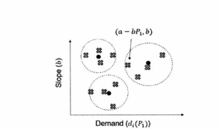
3.4.1 Generating the Demand Function Set . . . 61
3.4.2 Implementation Details . . . 64
3.4.3 Field Experiment Results . . . 65
4 An Adaptive Robust Optimization Approach to Supply Chain Risk Miti-gation 69 4.1 Overview and Summary of Results . . . 71
4.1.1 Related Literature . . . 73
4.2 The M odel . . . 74
4.2.1 Shortage Function . . . 75
4.2.2 Robust Optimization Model for Inventory Decision . . . 75
4.3 Optimization Algorithm . . . 76
4.3.1 Analysis of the Shortage Function . . . 77
4.3.2 Delayed Constraint Generation Algorithm . . . 78
4.4 Analysis for K-Chain Designs . . . 81
4.4.1 Total Inventory Required by K-chain . . . 82
4.4.2 Inventory Allocation Strategy . . . 84
4.5 Computational Experiments . . . 87
4.5.1 Balanced System Example . . . 87
4.6 Extensions . . . . 4.6.1 Different Holding Costs and Lost Sales Costs
4.6.2 Time-to-Survive Model . . . .
5 Concluding Remarks
5.1 Summary and Future Directions. 5.2 Overview of Dynamic Learning and
A Technical Results for Chapter 2 A.1 Proofs of Theorem 2.1 . . . .
A. 1.1 Preliminaries . . . . A.1.2 Proof of Theorem 2.1 . . . . A.2 Useful Facts . . . .
B Technical Results for Chapter 3 B.1 Proofs of the Results in Section 3.3
B.1.1 Proof of Theorem 3.3. . . . B.1.2 Proof of Lemma 3.7 . . . . B.1.3 Proof of Proposition 3.9 B. 1.4 Proof of Proposition 3.10 B.1.5 Proof of Proposition 3.12
C Technical Results for Chapter 4 C.1 Proofs . . . . C.1.1 Proof of Lemma 4.1 . . . . C.1.2 Proof of Lemma 4.2 . . C.1.3 Proof of Proposition 4.3 C.1.4 Proof of Lemma 4.7 . . . . C.1.5 Proof of Proposition 4.8 . . C.1.6 Proofs of Lemma 4.9 and 4.1 C.2 Computing D'(t) . . . . C.3 Type 1 Service Level . . . . C.4 Hardness Result . . . . C.5 Choosing Uncertainty Sets . . . . .
Optimization... 91 91 92 95 95 97 99 . . . 9 9 . . . 9 9 . . . 1 0 5 . . . 121 125 . . . 1 2 5 . . . 125 . . . 128 . . . 129 . . . 131 . . . 1 3 2 135 . . . 135 . . . 135 . . . 135 . . . 136 . . . 137 . . . 138 . . . 139 . . . 143 . . . 145 . . . 1 4 5 . . . 147 .0 . . . . . . . .
C.5.1 Structure of the Proposed Uncertainty Sets . . . 148 C.5.2 Selecting Parameters to Model Demand Uncertainty . . . 149
List of Figures
2-1 Performance Comparison of Dynamic Pricing Algorithms - Single Product
Exam ple . . . 37
2-2 Performance Comparison of Dynamic Pricing Algorithms - Single Product with Degenerate Optimal Solution . . . 38
2-3 Performance Comparison of Dynamic Pricing Algorithms - Multi-Product Exam ple . . . 40
2-4 Performance Comparison of Dynamic Pricing Algorithms - Contextual Example 44 3-1 Screenshot of A Restaurant Deal on Groupon's Website . . . 60
3-2 Applying K-means Clustering to Generate K Linear Demand Functions . . 62
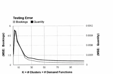
3-3 Mean Squared Error of Demand Prediction for Different Values of K . . . 64
3-4 Bookings and Revenue Increase by Deal Category . . . 66
4-1 Process Flexibility Designs . . . 70
4-2 Inventory under Asymmetric Demand in K-chains . . . 87
4-3 Flexibility Design in the Asymmetric Example . . . 89
4-4 Flexibility Design in the Asymmetric Example (continued) . . . 89
5-1 An Illustration of Open-Loop Decision Processes . . . 97
List of Tables
2.1 Literature on Dynamic Learning and Pricing with Limited Inventory . . . 23
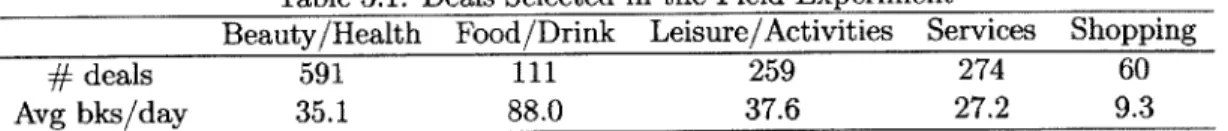
3.1 Deals Selected in the Field Experiment . . . .. . . . 65
4.1 Constraint Generation Algorithm for the Balanced System . . . 88
4.2 Inventory Allocation for Unbalanced System . . . 90
Chapter 1
Introduction
Operations management refers to the administration of business practices to convert re-sources into goods and services. It studies a broad range of operational decisions including the design and management of products, processes, services and supply chains.1 These op-erational decisions are often made in an uncertain environment. The uncertainty could rise from a variety of sources: randomness in production yield, disruptions in supply chains, and fluctuations in customer demand, etc.
In classical operations management literature, uncertainties are dealt with in two sepa-rate stages. In the first stage, the firm estimates some probability distribution from historical data using statistical tools, and use it to model uncertainty. In the second stage, the firm in-corporates the probability distribution into some decision models, and optimizes its decisions given that probability distribution. Therefore, under this framework, the estimation pro-cess is separated from the decision propro-cess. Indeed, most operations management literature assumes the probability distribution as given.
Over the past few years, there has been growing interest in combining estimation pro-cesses and decision propro-cesses in operations management. This new trend is driven by two forces: one is the advances in information technology, which enable the firm to quickly collect and process large amounts of data, so that the estimation process can be completed in real time. Another driving force is the popular business practice of reducing product life cycle in order to introduce new products more frequently. The short product life cycle means that there is less time to complete the estimation process and 'the decision process separately.
Therefore, many firms in fashion and online retail industries have adopted new approaches that integrate statistical learning into their decision processes.
To give an example, let us consider Groupon, a large e-commerce marketplace and a collaborator in this research. Groupon is a website where customers can purchase discount deals from local merchants. Every day, thousands of new deals are launched on Groupon's website. Deals are only available for limited time, ranging from several weeks to several months. Due to this business model, Groupon is faced with high level of demand uncertainty, mainly because there is no previous sales data for newly launched deals. This challenge presents an opportunity for Groupon to learn about customer demand using real time sales data after deals have been launched in order to obtain more accurate demand estimation.
Motivated by Groupon, this thesis considers several fundamental problems in opera-tions management with dynamic learning and optimization. The key challenge of dynamic learning, or online learning, is to address the exploration-exploitation tradeoff. Generally speaking, exploitation means optimizing the system using the current available data and greedy solutions. Exploration means collecting more data by deviating from the current greedy optimal decision in order to improve future decision.
In the following, we will first give a brief review of the general exploration-exploration theory, and then present its applications in two operations management areas: revenue
management and supply chain management.
1.1
Background
1.1.1 Exploration-Exploitation Tradeoff
Multi-armed bandit is a classical problem that models the essence of exploration-exploitation tradeoff. It was first proposed by Thompson (1933), who is motivated by clinical trials, and formally formulated by Robbins (1952). The basic problem is as follows: there are multiple slot machines in a casino, and there is a gambler who has finite number of tokens. The name "one-armed bandit" refers to the colloquial term of a slot machine, hence the model setting is called a "multi-armed bandit." With each token, the gambler can play any arm. The reward from each arm is i.i.d., but their reward distribution is unknown to the gambler. Therefore, the gambler needs to sequentially allocates tokens to different slot machines in order to learn their distributions. The goal is to maximize the total expected reward.
The multi-armed bandit problem has numerous variants. For example, one variant is called "continuous bandit" or "continuum bandit": Instead of finitely many arms, there are infinitely many arms indexed by a continuous interval, see Kleinberg and Leighton (2003), Mersereau et al. (2009), Rusmevichientong and Tsitsiklis (2010). Another variant is known as "contextual bandit," where the decision maker receives some external information that can help predict the reward distribution at the beginning of each round.
We will further discuss the multi-armed bandit literature in the subsequent chapters.
1.1.2 Dynamic Pricing and Online Demand Learning
The multi-armed bandit model can be used for dynamic pricing in the setting of incomplete demand information. In this setting, the firm has to learn about the demand model while changing price in real time. One can view each price as an "arm" of the bandit, and the revenue under that price as the "reward" associate with that "arm." This analogy builds a
direct connection between multi-armed bandit problems and dynamic pricing problems. Joint learning-and-pricing problems have received extensive research attention over the last decade. Recent surveys by Aviv and Vulcano (2012) and den Boer (2015) provide a comprehensive overview of this area. Recent revenue management papers that consider price experimentation for learning demand curves include Besbes and Zeevi (2009), Boyaci and Ozer (2010), Wang et al. (2014) and Besbes and Zeevi (2015). Another stream of papers focuses on semi-myopic pricing policies using various learning methods. Examples include maximum likelihood estimation (Broder and Rusmevichientong 2012), Bayesian methods (Harrison et al. 2012), maximum quasi-likelihood estimation (den Boer and Zwart 2014, den Boer 2014) and iterative least-squares estimation (Keskin and Zeevi 2014).
In most of these papers, the dynamic pricing models deviate from the classical multi-armed bandit model because the seller can choose price from a continuous interval (and hence a "continuum bandit"). Another practical issue is that the classical multi-armed bandit model does not include the inventory constraint, while many sellers is faced with limited inventory. These issues will be further discussed in Chapter 2 and 3.
1.1.3 Adaptive Supply Chain Risk Mitigation
A key idea in the multi-armed bandit problem is to make decisions sequentially so that future decisions can be adaptive to newly revealed information. We further exploit this
idea in the setting of supply chain risk mitigation. More specifically, we consider a hybrid strategy using both ex-ante decisions (i.e., inventory) and ex-post decisions (i.e., flexibility). The ex-post decisions of this strategy are made adaptively after disruptions happen.
There is a rich literature on risk mitigation using inventory. Many of the earlier papers (e.g., Meyer et al. 1979, Song and Zipkin 1996, Arreola-Risa and DeCroix 1998) studied inventory risk mitigation in a single product setting. More recently, inventory mitigation strategies under multi-period, multi-echelon settings have also been considered (e.g., Bol-lapragada et al. 2004, DeCroix 2013). However, a main drawback of using inventory alone is that it may require too much inventory to achieve a satisfiable service level.
Process flexibility, also referred to as "mix flexibility" or "product flexibility," has also been observed as potential risk mitigation tool. Tomlin and Wang (2005) considers a risk mitigation strategy that uses a combination of mix-flexibility and dual sourcing. Tang and Tomlin (2008) suggests process flexibility as one of the five types of flexibility strategies that can be used to mitigate supply chain disruptions. And finally, Sodhi and Tang (2012) lists flexible manufacturing processes as one of the eleven robust supply chain strategies.
In this thesis, we propose a hybrid approach to study the risk mitigation strategy by combining both flexibility and inventory. This idea is partially studied by Giirler and Parlar (1997), Tomlin (2006) in the dual sourcing setting. The hybrid strategy requires the firm to allocate inventory before the uncertainties (ex-ante), and to adjust its production level after uncertainties are realized (ex-post). We will further discuss this problem in Chapter 4.
1.2
Overview
The remaining parts of this thesis are organized as follows.
In Chapter 2, we consider a network revenue management problem where an online re-tailer aims to maximize revenue from multiple products with limited inventory constraints. We propose a dynamic learning and pricing algorithm, which builds upon the Thompson sampling algorithm used for multi-armed bandit problems by incorporating inventory con-straints.
In Chapter 3, we consider a dynamic pricing problem for a single product where the demand curve is not known a priori. We explicitly consider a business constraint, which prevents the seller from conducting extensive price experimentation. Our analysis provides
important structural insights into the optimal pricing strategies. In addition to the theoreti-cal results, we will describe an implementation at Groupon, a large e-commerce marketplace for daily deals.
In Chapter 4, we study a supply chain risk management problem by considering a hybrid strategy that uses both (process) flexibility and inventory. The interplay between process flexibility and inventory is modeled as a two-stage robust optimization problem. We develop a delayed constraint generation algorithm that can efficiently solve the two-stage robust optimization problem.
Finally, we provide some concluding remarks in Chapter 5. The technical proofs for each chapter are included in the appendices.
Chapter 2
Online Network Revenue
Management with Thompson
Sampling
In this chapter, we focus on a classical revenue management problem: A retailer is given an initial inventory of resources and a finite selling season. Inventory cannot be replenished throughout the season. The firm must choose prices for a set of products to maximize revenue over the course of the season, where each product consumes certain amount of resource inventory. The retailer has the ability to observe consumer purchase decisions in real-time and can dynamically adjust the price at negligible cost.
For historical reason, this problem is known as the network revenue management prob-lem, because it was first proposed by Gallego and Van Ryzin (1997) for the airline network yield management problem. In the airline setting, each "product" is an itinerary path from an origin to a destination, and each "resource" is a single flight leg in the network.
The network revenue management problem has been well-studied in the academic litera-ture under the additional assumption that the mean demand rate associated with each price is known to the retailer prior to the selling season. In practice, many retailers do not know the exact mean demand rates; thus, we focus on the network revenue management problem with unknown demand.
Given unknown mean demand rates, the retailer faces a tradeoff commonly referred to as the exploration- exploitation tradeoff (see Section 1.1.1). In the network revenue management
setting, the retailer is constrained by limited inventory and thus faces an additional tradeoff. Specifically, pursuing the exploration objective comes at the cost of diminishing valuable inventory. Simply put, if inventory is depleted while exploring different prices, there is no inventory left to exploit the knowledge gained.
We develop an algorithm for the network revenue management setting with unknown mean demand rates which balances the exploration-exploitation tradeoff while also incorpo-rating inventory constraints. Our algorithm is based on the Thompson sampling algorithm for the stochastic multi-armed bandit problem, where we add a linear program (LP) sub-routine to incorporate inventory constraints. The proposed algorithm is easy to implement and also has strong performance guarantees. The flexibility of Thompson sampling allows our algorithm to be generalized to various extensions. More broadly, our algorithm can be viewed as a way to solve multi-armed bandit problems with resource constraints. Such problems have wide applications in dynamic pricing, dynamic online advertising, and crowd-sourcing Badanidiyuru et al. (2013).
2.1
Literature Review
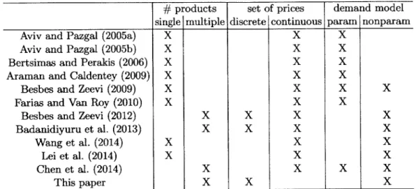
Due to the increased availability of real-time demand data, there is growing academic interest on dynamic pricing problems using a demand learning approach. Section 1.1.2 gave a general overview of this research area. The review below is focused on existing literature that considers inventory constraints. In Table 2.1, we list research papers that address limited inventory constraints and classify their models based on the number of products, allowable price sets being discrete or continuous, and whether the demand model is parametric or non-parametric.
As described earlier, our work generalizes to the network revenue management setting, thus allowing for multiple products, whereas much of the literature is for the single product setting.
The papers included in Table 2.1 propose pricing algorithms that can be roughly divided into three groups. The first group consider joint learning and pricing problem using dynamic programing (DP) Aviv and Pazgal (2005a,b), Bertsimas and Perakis (2006), Araman and Caldentey (2009), Farias and Van Roy (2010). The resulting DP is usually intractable due to high dimensions, so heuristics are often used in these papers. Since the additional inventory
#
products set of prices demand modelsingle multiple discrete continuous param nonparam
Aviv and Pazgal (2005a) X X X
Aviv and Pazgal (2005b) X X X
Bertsimas and Perakis (2006) X X X
Araman and Caldentey (2009) X X X
Besbes and Zeevi (2009) X X X X
Farias and Van Roy (2010) X X X
Besbes and Zeevi (2012) X X X X
Badanidiyuru et al. (2013) X X X X
Wang et al. (2014) X X X
Lei et al. (2014) X X X
Chen et al. (2014) X X X X
This paper X X X
Table 2.1: Literature on Dynamic Learning and Pricing with Limited Inventory
constraints add to the dimension of DPs, papers in this group almost exclusively consider single product settings in order to limit the complexity of the DPs.
The second group applies a simple strategy that separates the time horizon into a de-mand learning phase (exploration objective) and a revenue maximization phase (exploitation objective) Besbes and Zeevi (2009, 2012), Chen et al. (2014). Recently, Wang et al. (2014), Lei et al. (2014) show that when there is a single product, pricing algorithms can be im-proved by mixing the exploration and exploitation phases. However, their methods cannot be generalized beyond the single-product/continuous-price setting.1
The third group of papers builds on the classical multi-armed bandit algorithms (Badani-diyuru et al. (2013) and this paper) or the stochastic approximation methods Besbes and Zeevi (2009), Lei et al. (2014). The multi-armed bandit problem is often used to model the exploration-exploitation tradeoff in the dynamic learning and pricing model without lim-ited inventory constraints; see Gittins et al. (2011), and Bubeck and Cesa-Bianchi (2012) for an overview of this problem. Thompson sampling is a powerful algorithm used for the multi-armed bandit problem, and it is a key building block of the algorithm that we propose.
Thompson sampling. In one of the earliest papers on the multi-armed bandit problem, Thompson (1933) proposed a randomized Bayesian algorithm, which was later referred to
as Thompson sampling. The basic idea of Thompson sampling is that at each time period,
'Lei et al. (2014) also consider a special case of multi-product setting where there is no cross-elasticity in product demands.
random numbers are sampled according to the posterior probability distributions of the reward of each arm, and then the arm with the highest sampled reward is chosen. The algorithm is also known as probability matching since the probability of an arm being chosen matches the posterior probability that this arm has the highest expected reward. Compared to other popular multi-armed bandit algorithms such as those in the Upper Confidence Bound (UCB) family Lai and Robbins (1985), Auer et al. (2002a), Garivier and Capp6 (2011), Thompson sampling enjoys comparable theoretical performance guarantees Agrawal and Goyal (2011), Kaufmann et al. (2012), Agrawal and Goyal (2013) and better empirical performance Chapelle and Li (2011). In addition, the Thompson sampling algorithm shows great flexibility and has been adapted to various model settings Russo and Van Roy (2014). We believe that a salient feature of this algorithm's success is its ability to update mean demand estimation in every period and then exploit this knowledge in subsequent periods. As you will see, we take advantage of this property in our development of a new algorithm for the network revenue management problem when demand distribution is unknown.
2.2
Model
We consider a retailer who sells N products, indexed by i = 1,..., N, over a finite selling
season. These products consume M limited resources, indexed by j - 1,. . . , M. Specifically,
one unit of product i consumes
aij
units of resource j, which has Ij units of initial inventory. There is no replenishment during the selling season.The selling season is divided into T periods. In each period t = 1, ... T, the retailer
offers a price vector P(t) = [P1(t),..., PN(t)], where P(t) is the price for product i at
period t. We use P to denote the admissible price set. After the retailer chooses P(t) E
P,
customers observe the price vector chosen and make purchase decisions. We use vectorD(t) = [DI(t), ... , DN(t)] to denote the realized demand at period t.
1. If there is inventory available to satisfy demand for all products, then the retailer receives revenue Ef_ Di(t)P(t). Inventory is depleted by EN_
1
Di(t)aij for eachresource
j
= 1, .. ., M.2. If there is not enough resource available to satisfy demand for some products, demand for those products is lost. In our analysis, we assume that the selling season immedi-ately ends when there is a lost demand. Since we are aiming at a lower bound of the
retailer's expected revenue, this simplification does not change the result.
We assume that demand is only affected by the current price, and is not affected by previous or future prices. The joint demand distribution per period under price p E P is denoted by F(p, 9), where 9 E
e
is some parameter. The mean demand under distributionF(p, 0) is denoted by d(p, 9) = [d,(p, 0), . .. , dN(p, 0)]. By assuming the joint distribution F(., 9), demand for different products or demand under different prices can be correlated.
The true parameter 0 is unknown the retailer, and the estimates of 9 are updated in a Bayesian fashion. We denote by H(t) the history (P(1), D(1), ... , P(t), D(t)). The posterior
distribution of 9 given the history is P( E - I H(t)). The retailer's goal is to choose price
vector P(t) sequentially to maximize revenue over the course of the selling season.
In the following, we present several special cases based on demand models that are widely used in practice.
2.2.1 Discrete Price Case
In many practical cases, the price set consists of finite number of price vectors: P =
{P1,. . . , PK}. Here, each p E P is a N-dimensional vector, specifying the price for each of the N products.
Nonparametric Demand Model
We assume an independent prior: F(pk, 0) = lIFi(pk, Oik). Based on this prior, we can update the demand for each product under each price separately.
Note the assumption of the independent prior that does not restrict the true demand distribution to be independent across different products and different prices. In fact, the true demand distribution can have arbitrary correlation and dependence between prices and products. Imposing an independent prior simply means that we update the marginal demand for each product under each price separately. Therefore, this approach is "nonparametric"
in that it does not impose any restrictive assumptions on the demand correlation.
Multi-armed Bandit with Global Constraints
The discrete price model can also be used to model a multi-armed bandit problem with global resource constraints. The problem is also known as "bandits with knapsacks" in
Badanidiyuru et al. (2013).
The problem is the following: there are multiple arms (k = 1,... , K) and multiple
resources (j = 1,... , M). At each time period t = 1,. . ., T, the decision maker chooses
to pull one of the arms. If arm k is pulled, it generates a Bernoulli variable with mean
0k, which is unknown to the decision maker. If the generated value is one, the decision
maker consumes bjk units of resource
j;
in addition, the decision maker receives rk units of reward. If the generated value is zero, no resource is consumed and no reward is received. (More generally, if resource consumptions and rewards in each period are not binary but have bounded probability distributions, we can reduce the problem to the one with binary distributions using the re-sampling trick described in Section 2.3.1.) At any given time, if there exists j = 1,..., l such that the total consumption of resourcej
up to this time is greater than a fixed constant Ij, the decision process immediately stops and no future rewards will be received.To see show that this problem is a special case of our model, we can consider a set of products indexed by k = 1, ... , K. The price set is discrete: P = {PI, ... , pK}, where
choosing price P means only offering product k at price rk, while making other products unavailable. The mean demand for product k is Ok, and the resource consumption coefficient is akj = bkj.
In line with standard terminology in the multi-armed bandit literature, we will refer to "pulling arm k" as the retailer "offering price Pk", and "arm k" will be used interchangeably
with "price P".
The presence of inventory constraints significantly complicates the problem, even for the special case of a single product. In the classical multi-armed bandit setting, if success probability of each arm is known, the optimal strategy is to choose the arm with the highest mean reward. But in the presence of limited inventory, a mixed strategy that chooses multiple prices over the selling season may achieve higher revenue than any single price strategy. Therefore, a reasonable strategy for the multi-armed bandit model with global constraint should not converge to the optimal single price, but to the optimal distribution of (possibly) multiple prices. Another challenging task is to estimate the time when inventory runs out and the selling season ends early, which is itself a random variable depending on the chosen strategy. Such estimation is necessary for computing the expected reward. This is opposed to classical multi-armed bandit problems for which algorithms always end at a
fixed period.
Display Advertising Example. To show an application of the multi-armed bandit model with global constraint, we consider an example of placing online ads. Suppose there is an online ad platform (e.g. Google) that uses the pay per click system. For each user logging on to a third-party website, Google may display a banner ad on the website. If the user clicks the ad, the advertiser sponsoring the ad pays some amount of money that is split between Google and the website hosting the banner ad (known as the publisher). If the user does not click the ad, no payment is made. Assuming that click rates for ads are unknown, Google faces the problem of allocating ads to publishers to maximize its revenue, while satisfying advertisers' budgets.
This problem fits into the limited resource multi-armed bandit model as follows: each arm is an ad, and each resource corresponds to an advertiser's budget. If ad k is clicked, the advertiser
j
sponsoring ad k pays bjk units from its budget, of which Google gets a splitof rk.
Note that this model is only a simplified version of the real problem. In practice, Google also obtains some data about the user and the website (e.g. the user's location or the website's keywords) and is able to use this information to improve its ad display strategy. We consider such an extension with contextual information in Section 2.6.
2.3
Thompson Sampling Algorithm with Limited Inventory
In this section, we propose an algorithm called "Thompson Sampling with Limited Inventory" that builds off the original Thompson sampling algorithm Thompson (1933) to incorporate inventory constraints.
For convenience, we first define a "dummy price", p,, where di(p,,
6)
= 0 for all i = 1,... IN and 0E
9. We define X as the set of all probability distribution over P U {po}. For any x E X, which is a probability measure over P U {p}, we leti
be the corresponding normalized probability measure overP.
That is, for any subsetP'
CP,
we have i(P') =X p') /X th
Algorithm 1 Thompson Sampling with Inventory (TS-general) The retailer starts with inventory level Ij (0) = Ij for all
j
= 1,..., M. Repeat the following steps for all t = 1, ... , T:1. Sample Demand: sample Ot from P(0 E j H(t - 1)). 2. Optimize: Solve the following optimization problem:
N
f(O(t)) = max Ep.X[Epidi(p, 0(t))]
i1
N
subject to Ex[Z aijdi(p, 0(t))] I,/T for all
j
= 1,..., MLet x(t) be its optimal solution, and
z(t)
be the corresponding normalized distribution over P.3. Offer Price: Retailer chooses price vector P(t) E P according to probability distribu-tion i(t).
4. Update: Customer's purchase decisions, D(t), are revealed to the retailer. The retailer updates the history H(t) = H(t - 1) U {P(t), D(t)} and the posterior distribution of 0, P(O E - I H(t)). The retailer also updates inventory level I(t) = I(t - 1)
-):N Di(t)aij for all j = 1, ... , M.
2.3.1 Special Cases of the Algorithm
Discrete Price, Bernoulli Demand We consider a special case where there are finitely many prices: P = {p1, ... ,PK}. Demands for each product are Bernoulli random variables. Let Nk(t - 1) be the number of time periods that the retailer has offered price PA in the first t - 1 periods, and let Wik(t - 1) be the number of periods that product i is purchased under price Pk during these periods. Define Ij (t - 1) as the remaining inventory of resource
j
at the beginning of the tth time period. Define constants cj = I /T for resourcej,
whereIj= I(0) is the initial inventory level.
The model defined in Section 2.2.1 allows for any joint demand distribution F(p, 0). However, to avoid misspecification of the demand model, we consider a Bayesian updating process which only updates the marginal demand distribution under the chosen price. We present this process in Algorithm 2.
In Algorithm 2, steps 1 and 4 are based on the Thompson sampling algorithm for the classical multi-armed bandit setting. In particular, in step 1, the retailer randomly samples product demands according to demand posterior distribution. In step 4, upon observing customer purchase decisions, the retailer updates the posterior distributions under the chosen price. We use Beta posterior distributions in the algorithm-a common choice in Thompson sampling-because the Beta distribution is conjugate to Bernoulli random variables. The posterior distributions of the unchosen price vectors are not changed.
The algorithm differs from the ordinary Thompson sampling algorithm in steps 2 and 3. In step 2, instead of choosing the price with the highest reward using sampled demand, the retailer first solves a linear program (LP) which identifies the optimal mixed price strategy that maximizes expected revenue given sampled demand. The first constraint specifies that the average resource consumption per time period cannot exceed the initial inventory divided by length of the time horizon. The second constraint specifies that the sum of the probabilities of choosing all price vectors cannot exceed one. In step 3, the retailer randomly offers one of the K price vectors according to probabilities specified by the LP's optimal solution. Note that if all resources have positive inventory levels, we have Ek_ 1
xk(t)
> 0 in the optimal solution to the LP, so the probabilities are well-defined.In the remainder of the paper, we use TS-fixed as an abbreviation for Algorithm 2. The term "fixed" refers to the fact that the algorithm uses a fixed inventory to time ratio
Algorithm 2 Thompson Sampling with Inventory (TS-fixed)
Repeat the following steps for all t = 1, ... , T:
1. Sample Demand: For each price k and each product i, sample Oik(t) from a
Beta(Wik(t - 1) + 1, Nk(t - 1) - Wik(t - 1) + 1) distribution. 2. Optimize: Solve the following linear program, OPT(6)
K N
f (0) = max Z(ZpikOik(t))xk k=1 i=1
K N
subject to Z(Z aijOik(t))xk cj for allj=1,...,AiM
k=1 i=1
K
Zxk < 1 k=1
xk > 0, for all k =1. K
Let x(t) = (x1(t), XK(t)) be the optimal solution to OPT(O) at time t. 3. Offer Price: Retailer chooses price vector P(t) = Pk with probability
K
k=1
4. Update: Customer's purchase decisions, D(t), are revealed to the retailer. The retailer
sets Nk(t) = Nk(t -1) + 1, Wik(t) = Wik(t -1) + Di(t) for all i = 1, ... , N, and
1 (t) = I,(t - 1) - E=1 Di(t)aij for all j = 1,..., M.
ci = Ij/T in the LP for every
period.-Inventory Updating Intuitively, improvements can be made to the TS-fixed algorithm by incorporating the real time inventory information. In particular, we can change cj = I/T
to cj(t) = I(t - 1)/(T - t+1) in the LP in step 2. This change is shown in Algorithm 3. We refer to this modified algorithm as the "Thompson Sampling with Inventory Rate Updating algorithm" (TS-update, for short).
Algorithm 3 Thompson Sampling with Inventory Rate Updating (TS-update) Repeat the following steps for all t = 1, ... , T:
" Perform step 1 in Algorithm 1.
" Optimize: Solve the following linear program, OPT(O) K N
f (0) = max Z( pik2xk(t))xk
Xk k=1 i=1
K N
subject to
Z(Z
ajjOik(t))xk < c,(t) for all j = 1, . .,AIk=1 i=1
K
)x 1
k=1
Xk > 0, for all k =1,...,K
" Perform steps 3-5 in Algorithm 1.
In the revenue management literature, the idea of using updated inventory rates, cj(t), has been studied under the assumption that the demand distribution is known Secomandi (2008), Jasin and Kumar (2012). Recently, Chen et al. (2014) consider a pricing policy using updated inventory rates in the unknown demand setting. In practice, using updated inventory rates usually improves revenue compared to using fixed inventory rates cj Talluri and van Ryzin (2005). We also show in Section 2.5 that TS-update outperforms TS-fixed in simulations. Unfortunately, since TS-update involves a randomized demand sampling step, theoretical performance analysis of this algorithm appears to be much more challenging than TS-fixed and other algorithms in the existing literature.
General Demand Distributions with Bounded Support If di(pk) is randomly dis-tributed with bounded support [dik 1dik], we can reduce the general distribution to a
two-point distribution, and update it with Beta priors as in Algorithm 2. Suppose the retailer observes random demand Di(t) E [dik, dikl- We then re-sample a new random number, which equals to dik with probability (di - Di()/(k - dik) and equals to dik with probability (Di(t) - dik)/(dik - dik). It is easily verifiable that the re-sampled demand has the same mean as the original demand.2 By using re-sampling, the theoretical results in Section 2.4 also hold for the bounded demand setting.
As a special case, if demands have multinomial distributions for all i = 1, . , N and
k = 1, ... , K, we can use Beta parameters similarly as in Algorithm 2 without resorting to
re-sampling. This is because the Beta distribution is conjugate to the multinomial distribution.
Poisson Demand Distribution If the demand follows a Poisson distribution, we can use the Gamma distribution as the conjugate prior; see Algorithm 4. We use Gamma(a, A) to represent a Gamma distribution with shape parameter ce and rate parameter A.
Algorithm 4 Thompson Sampling with Poisson Demand Repeat the following steps for all t = 1, ... , T:
" Sample Demand: For each price k and each product i, sample Oik (t) from a
Gamma(Wik(t - 1) + 1, Nk (t - 1) + 1) distribution.
* Optimize: Solve the linear program, OPT(9), used in either Algorithm 2 or Algo-rithm 3.
" Perform steps 3-5 in Algorithm 1.
Note that Poisson demand cannot be reduced to the Bernoulli demand setting by the re-sampling method described above because Poisson demand has unbounded support. Note that Besbes and Zeevi (2012) assume that customers arrive according to a Poisson distri-bution, so when we compare our algorithm with theirs in Section 2.5, we use this variant of our algorithm.
2.4
Theoretical Analysis
In this section, we present a theoretical analysis of the TS-fixed algorithm. We consider a scaling regime where the initial inventory Ij increases linearly with the time horizon T for
all resources
j
= 1, .. ., M. Under this scaling regime, the average inventory per time period 2Cj =
I/T
remains constant. This scaling regime is widely used in revenue management literature.2.4.1 Benchmark and Linear Programming Relaxation
To evaluate the retailer's strategy, we compare the retailer's revenue with a benchmark where the true demand distribution is known a priori. We define the retailer's regret as
Regret(T) = E[R*(T)] - E[R(T)],
where R* (T) is the optimal revenue if the demand distribution is known a priori, and R(T) is the revenue when the demand distribution is unknown. In words, the regret is a non-negative quantity measuring the retailer's revenue loss due to not knowing the latent demand.
Because evaluating the expected optimal revenue with known demand requires solving a dynamic programming problem, it is difficult to compute the optimal revenue exactly even for moderate problem sizes. Gallego and Van Ryzin (1997) show that the expected optimal revenue can be approximated by the following upper bound. Let xk be the fraction of periods that the retailer chooses price Pk for k = 1,.. ., K. The upper bound is given by the following deterministic LP, denoted by OPTTB:
K N
f= max ipkdi(pk))xk
k=1 i=1
K N
subject to
Z(Z
aijdi(pk))xk 5 cj for all j = 1, Mk=1 i=1
K
Xk <1 k=1
Xk > 0, for all k = 1,...,K.
Recall that di(pk) is the expected demand of product i under price pk. Problem OPTB is almost identical to the LP used in step 2 of TS-fixed, except that it uses the true mean demand instead of sampled demand from posterior distributions. We denote the optimal value of OPTUB as
f*
and the optimal solution as (x*,..., x*). A well-known result inGallego and Van Ryzin (1997) shows that
E[R*(T)I f*T.
In addition, if the retailer chooses prices according to probability distribution (X, ... ,
x*1)
at each time period, the expected revenue is within O(v71) of the upper bound f*T.2.4.2 Analysis of Thompson Sampling with Inventory Algorithm
We now prove the following regret bound for TS-fixed.
Theorem 2.1. Suppose that the optimal solution(s) of OPTUB are non-degenerate. If the
demand distribution has bounded support, the regret of TS-fixed is bounded by
Regret(T) O(Vlog T log log T).
Proof Sketch. The complete proof of Theorem 2.1 can be found in Appendix A. We start
with the case where there is a unique optimal solution, and the proof has three main parts. Suppose X* is the optimal basis of OPTUB. The first part of the proof shows that
TS-fixed chooses arms that do not belong to X* for no more than
O(v/iilog
T) times. Thenin the second part, assuming there is unlimited inventory, we bound the revenue when only arms in X* are chosen. In particular, we take advantage of the fact that TS-fixed performs continuous exploration and exploitation, so the LP solution of the algorithm converges to the optimal solution of OPTUB. In the third part, we bound the expected lost sales due to having limited inventory, which should be subtracted from the revenue calculated in the second part. The case of multiple optimal solutions is proved along the same line. E
Note that the non-degeneracy assumption of Theorem 2.1 only applies to the LP with the true mean demand, OPTUB. The theorem does not require that optimal solutions to
OPT(O), the LP that the retailer solves at each step, to be non-degenerate. Moreover, the
simulation experiments in Section 2.5 show that TS-fixed performs well even if the non-degeneracy assumption does not hold.
It is useful to compare the results in Theorem 2.1 to the regret bounds in Besbes and Zeevi (2012) and Badanidiyuru et al. (2013), since our model settings are essentially the same. Our regret bound improves upon the O(T3) bound proved in Besbes and Zeevi (2012) and
matches (omitting log factors) the O(VTT) bound in Badanidiyuru et al. (2013). We believe that the reason why our algorithm and the one proposed in Badanidiyuru et al. (2013) have stronger regret bounds is that they both perform continuous exploration and exploitation, whereas the algorithm in Besbes and Zeevi (2012) separates periods of exploration and exploitation.
However, we should note that the regret bound in Theorem 2.1 is problem-dependent, whereas the bounds in Besbes and Zeevi (2012) and Badanidiyuru et al. (2013) are
problem-independent. More specifically, we show that TS-fixed or TS-update guarantees Regret(T) <
CVT
]
log T log log T, where the constant C is a function of the demand data. As a result, the retailer cannot compute the constant C a priori since the mean demand is unknown. In contrast, the bounds proved in Besbes and Zeevi (2012) and Badanidiyuru et al. (2013) are independent of the demand data and only depend on parameters such as the number of price vectors or the number of resource constraints, which are known to the retailer. Moreover, the regret bounds in Besbes and Zeevi (2012) and Badanidiyuru et al. (2013) do not require the non-degeneracy assumption.It is well-known that the problem-independent lower bound for the multi-armed bandit problem is Regret(T) > Q(v7) Auer et al. (2002b). Since the multi-armed bandit problem can be viewed as a special case of our setting where inventory is unlimited, the algorithm in Badanidiyuru et al. (2013) has the best possible problem-independent bound (omitting log factors). The f(v7) lower bound is also proved separately by Besbes and Zeevi (2012) and Badanidiyuru et al. (2013).3 On the other hand, it is not clear what the problem-dependent
lower bound is for our setting, so we do not know for sure if our O(VT) problem-dependent
bound (omitting log factors) can be improved.
2.5
Numerical Results
In this section, we first provide an illustration of the TS-fixed and TS-update algorithms for the setting where a single product is sold throughout the course of the selling season, and we compare these results to other proposed algorithms in the literature. Then we present results for a multi-product example; for consistency, the example we chose to use is identical
3
Badanidiyuru et al. (2013) proves a more general lower bound where the initial inventory is not required to scale linearly with time T. However, one can show that their bound becomes Q(/T) under the additional assumption that inventory is linear in T.
to the one presented in Section 3.4 of Besbes and Zeevi (2012).
2.5.1 Single Product Example
Consider a retailer who sells a single product (N = 1) throughout a finite selling season. Without loss of generality, we can assume that the product is itself the resource (M = 1) which has limited inventory. The set of feasible prices is {$29.90, $34.90, $39.90, $44.90}, and the mean demand is given by d($29.90) = 0.8, d($34.90) = 0.6, d($39.90) = 0.3, and
d($44.90) = 0.1. As aligned with our theoretical results, we show numerical results when
inventory is scaled linearly with time, i.e. initial inventory I = aT, for a = 0.25 and 0.5. We evaluate and compare the performance of the following five dynamic pricing algo-rithms which have been proposed for our setting:
" TS-update: intuitively, this algorithm outperforms TS-fixed and is thus what we suggest for retailers to use in practice.
" TS-fixed: this is the algorithm we have proposed with strong regret bounds as shown in Section 2.4.
" The algorithm proposed in Besbes and Zeevi (2012): we implemented the algorithm with T= T2/3 as suggested in their paper, and we used the actual remaining inventory after the exploration phase as an input to the optimization problem which sets prices for the exploitation phase.
" The PD-BwK algorithm proposed in Badanidiyuru et al. (2013): this algorithm is based on the primal and the dual of OPTUB. For each period, it estimates upper bounds of revenue, lower bounds of resource consumption, and the dual price of each resource, and then selects the arm with the highest revenue-to-resource-cost ratio.
" Thompson sampling (TS): this is the algorithm described in Thompson (1933) which has been proposed for use as a dynamic pricing algorithm but does not consider in-ventory constraints.
We measure performance as the average percent of "optimal revenue" achieved over 500 simulations. By "optimal revenue", we are referring to the upper bound on optimal revenue where the retailer knows the mean demand at each price prior to the selling season; this
I
upper bound is the solution to OPTB, f*T, described in Section 2.4.1. Thus, the percent of optimal revenue achieved is at least as high as the numbers shown. Figure 2-1 shows performance results for the five algorithms outlined above.
Percent of Optimal Revenue Achieved I = 0.25T 00% 90% 85O4, ... ..- . 80%. 75%. 70% 100 1000 100 Number of Periods (T) I = 0.5T 100% 95% -....- -90%* 85% 75% -70% 100
a-- TS-update TS-fixed ---- + --- Badanidiyuru et al. (2013) - --- TS
Figure 2-1: Performance Comparison of Dynamic Pricing ample
1000
Number of Periods (T)
- Besbes & Zeevi (2012)
10000
Algorithms - Single Product
Ex-The first thing to notice is that all four algorithms that incorporate inventory constraints converge to the optimal revenue as the length of the selling season increases. The TS algo-rithm, which does not incorporate inventory constraints, does not converge to the optimal revenue. This is because in each of the examples shown, the optimal pricing strategy is a mixed strategy where two prices are offered throughout the selling season as opposed to a single price being offered to all customers. The optimal strategy when I = 0.25T is to offer the product at $39.90 to
4
of the customers and $44.90 to the remaining - of the customers. The optimal strategy when I = 0.5T is to offer the product at $34.90 to 2 of the customers and $39.90 to the remaining 1 of the customers. In both cases, TS converges to the suboptimal price $29.90 offered to all the customers since this is the price that max-imizes expected revenue given unlimited inventory. This really highlights the necessity of incorporating inventory constraints when developing dynamic pricing algorithms.Overall, TS-update outperforms all of the other algorithms in both examples. Interest-ingly, when considering only those algorithms that incorporate inventory constraints, the gap
I
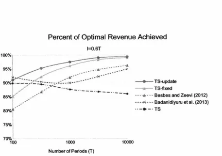
Percent of Optimal Revenue Achieved I=0.6T 100% 95%. 9--x - TS-update TS-fixed
85% Besbes and Zeevi (2012)
- -- -- Badanidiyuru et al. (2013) 80% ~ TS 75%. 70% 100 1000 10000 Number of Periods (T)
Figure 2-2: Performance Comparison of Dynamic Pricing Algorithms - Single Product with Degenerate Optimal Solution
between TS-update and the others generally shrinks when (i) the length of the selling season increases, and (ii) the ratio ]/T increases. This is consistent with many other examples that we have tested and suggests that our algorithm is particularly powerful (as compared to the others) when inventory is very limited and the selling season is short. In other words, our algorithm is able to more quickly learn mean demand and identify the optimal pricing strategy, which is particularly useful for low inventory settings.
We then perform another experiment when the optimal solution to OPTun is degenerate. We assume the initial inventory is I = 0.6T, so the degenerate optimal solution is to offer the product at $34.90 to all customers. Note that the degenerate case is not covered in the result of Theorem 2.1. Despite the lack of theoretical support, Figure 2-2 shows that TS-fixed and TS-update still perform well.
2.5.2 Multi-Product Example
Now we consider the example presented in Section 3.4 of Besbes and Zeevi (2012) where a retailer sells two products (N = 2) using three resources (1 = 3). Selling one unit
of product i =1 consumes 1 unit of resource j = 1, 3 units of resource j = 2, and
no units of resource
j
= 3. Selling one unit of product i= 2 consumes 1 unit of re-source 1, 1 unit of rere-source 2, and 5 units of rere-source 3. The set of feasible prices is(P1,P2) C {(1, 1.5), (1,2), (2,3), (4,4),(4,6.5)}. Besbes and Zeevi (2012) assume customers arrive according to a multivariate Poisson process. We would like to compare performance