Dynamic behavior of multi-legged pinned and rigid structural joints

(1)

DYNAMIC BEHAVIOR OF MULTI-LEGGED PINNED AND RIGID

STRUCTURAL JOINTS

by

Ronald L. Frink

Bachelor of Science Ocean Engineering Florida Institute of Technology (1984)

Submitted to the Department of Ocean Engineering in Partial Fulfillment of the Requirements

for the Degrees of

MASTER OF SCIENCE IN OCEAN ENGINEERING and MASTER OF SCIENCE IN MECHANICAL ENGINEERING at the

MASSACHUSETTS INSTITUTE OF TECHNOLOGY August, 1995

Signature of Author // I , ·

-Department of Ocean Engineering August, 1995

Certified by

Assistant Professor J. Robert Fricke artment of Ocean Engineering, Thesis Supervisor

Certified by

<'/ _{Assistant Pr essor Zaichun Feng}

Department of Mechanical Engineering, Thesis Reader

Accepted by ,N

-S,,,-

-:

~

Prolessor A.

D~

gaC

f ichael, Chairman

OF -r-!,. . oY _{Department Graduate Committee, Department of Ocean Engineering}

FEB 2 0 1997

.r- L

(2)

DYNAMIC BEHAVIOR OF MULTI-LEGGED PINNED AND RIGID

STRUCTURAL JOINTS

by

Ronald L. Frink

Submitted to the Department of Ocean Engineering on August 1, 1995 in partial fulfillment of the requirements for the degrees of

Master of Science in Ocean Engineering and Master of Science in Mechanical Engineering

Abstract

The objective of this thesis is to explore the dynamic response of three-legged structural joints to longitudinal impulse excitation. Three joints have been analyzed in the experimentation. One joint is pinned with spherical male legs whose surfaces are coated with Teflon. The spherical male legs of the second pinned-joint are coated with a visco-elastic interface. The third joint is rigid. The intent of the Teflon-coated joint is to model a frictionless pinned-joint and the intent of the joint with the visco-elastic interface is to gain insight into joint damping behavior.

A scattering matrix whose elements are transfer functions is introduced to assist in

understanding wave type coupling that occurs when an incident longitudinal wave scatters at each joint. Reciprocity has been used to determine other scattering matrix elements that could not be determined directly from experimentation. The experimental data has then been compared to analytical solutions from two-dimensional models; a two-dimensional analytical solution was used since generalized three-dimensional analytical solutions are not available.

The rigid joint exhibited relatively high levels of transmission for each wave type. Average transmission efficiency ranged between -7 to -34 dB. The rigid joint exhibited significant longitudinal transmission. The predicted transmission efficiency was, on the average, 30 dB lower than the experimental results. Three mechanisms are proposed which explain the failure of the analytical model to accurately predict the transmission efficiency. _{The Teflon-coated spherical pinned-joint offered significant transmission} reduction when compared to the rigid joint. It is only for narrow frequency bands and for few wave types where the rigid joint exhibits lower levels of transmission when compared to the Teflon-coated spherical pinned-joint. The spherical pinned-joint with the visco-elastic interface offered minimal overall transmission for all wave types. It is only for very narrow frequency bands and few wave types where either the rigid joint or the Teflon-coated joint exhibited lower levels of transmission. Flexural-to-longitudinal and longitudinal-to-flexural transmission efficiencies of -60 to -70 dB were observed for this joint at frequencies above 7.5 kHz. Longitudinal-to-longitudinal transmission efficiencies as low as -55 dB were also observed for the joint with the visco-elastic interface demonstrating a clear advantage for incorporating damping material into the design of a joint.

Thesis Supervisor: Dr. J. R. Fricke Title: Assistant Professor

(3)

Acknowledgments

I wish to extend my appreciation to Professor J. Robert Fricke and Professor Ira

Dyer. Without the funding and support you graciously provided, this wonderful

experience of being in academia once again would have been less pleasant and less

possible. I wish to thank the entire acoustics group administrative staff. Sabina, Taci and

Isela, I thank you for everything and truly appreciate the job that you so superbly perform.

I also thank Hua He for his thoughtful discussions and recommendations that often kept

me on the right path.

Most importantly, I thank my wonderful family. Mom, Pat, Ann, Mike, and Keith.

You are everything a son and brother could ask for. You have always been there

supporting and encouraging me and I thank you for letting me do the same for you. To all

my critters, Chris, Beth, Tim, Nathan and Ann Marie; I can only hope that I have been as

much an inspiration in your lives as you have been in mine. Your uncle loves you. I pray

that you will aspire to be honest, loving and giving. One day I will look up to all of you in

out-stretched arms and say, 'Thank you God for bringing me to this summit." I will not

get there alone! Be specific and committed to the vision of your dreams. Make them so.

At certain levels, our life is not our own. If you choose to live in a community,

have friends, ifyou _{have loved ones and you are loved, then you have entered an implicit}

and binding agreement. This agreement represents a willingness to take responsible

precautions to protect your life _{and therefore uphold the commitment to those who help}

give your life meaning and structure - the commitment to be here tomorrow, the next day

and the following so to allow the project of growth and community to continue, develop and move forwardfor the sake of future generations.

(4)

A bstract ... 2 Acknowledgments ... 3 Table of Contents ... 4 L ist of Figures ... 6 L ist of Tables ... 9 List of Symbols ... 11 Chapter 1 Introduction ... 14 1.1 Previous Research ... ... 16 1.2 Objective ... 16 1.3 Approach ... 17 Chapter 2 Apparatus ... 18 2.1 Joint Descriptions ... 18 2.2 Experimental Configuration ... 21

2.3 Data Acquisition Equipment ... 24

Chapter 3 Experimental Execution ... ... 27

3.1 Impulse Excitation ... ... 27

3.2 Windowing ... 27

Chapter 4 Scattering Matrix ... ₃₁

4.1 Principle ... ... 31

4.2 Joint Scattering Matrices ... 32

4.2.1 Joint 'A' Scattering Matrices ... 33

4.2.2 Joint 'B' Scattering Matrices ... 34

4.2.3 Joint 'C' Scattering Matrices ... 35

(5)

4.3.1 Transmission Function Derivation using the

Concept of Reciprocity ...

Chapter 5 Analytical Models and Predictions ...

5.1 Transmission from Flexural Wave Excitation ...

5.2 Transmission from Longitudinal Wave Excitation ...

Chapter 6 Experimental Results ...

6.1 Experimentally Determined Data ...

6.2 Data Determined by Reciprocity ...

6.3 Relative Joint Response ...

6.4 Scattering Matrix Elements Determined

Experim entally ... ...

6.5 Scattering Matrix Elements Determined by

R eciprocity ...

...

Chapter 7 Conclusion ...

...

7.1 Discussion of Results ...

7.2 Recommendations for Future Research ...

Appendix A

Appendix B

Appendix C

Appendix D

Appendix E

Bibliography

Joint 'A' Design ... ...

Joint 'B' Design ... ...

Joint 'C' Design ...

...

M atlab Code ... ...

Data Collection and Organization ...

37 41 41 44 46 46 51 52 59 72 82 82 83 86 91 105 107 114 118

(6)

List of Figures

2-1 Joint 'A' (Rigid Joint) ... 19

2-2 Joint 'B' (Spherical Pinned-Joint, Teflon coated contact surfaces) 20 2-3 Joint 'B' (top section, bottom section, and spherical male leg) ... 20

2-4 Laboratory experimental configuration ... 22

2-5 Static compressive loading configuration ... 23

2-6 Coordinate System ... 23

2-7 Accelerometer Configuration ... 25

2-8 Orientation of an accelerometer pair in a typical cross-section to measure wave types ... 25

2-9 Data acquisition equipment ... 26

3-1 Example of the windowing process for a typical incident longitudinal waveform (Leg 1) ... 29

3-2 Example of the windowing process for a typical transmitted longitudinal waveform (Leg 3) ... 30

5-1 Two-dimensional structural joint ... .. 41

5-2 Model of two-dimensional joint with stiffness, dissipation and m ass ... 42

6-1 Cross-section of the leg/joint interaction demonstrating radial oscillatory expansion and contraction ... 49

6-2 Cross-section of the leg/joint interaction demonstrating translational oscillatory behavior ... ... 49

6-3 Rigid Joint Scattering Matrix Elements b14 and b24 ... 60

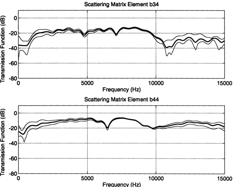
6-4 Rigid Joint Scattering Matrix Elements b34 and b44 ... 61

6-5 Rigid Joint Scattering Matrix Elements c14 and c24 ... 62

6-6 Rigid Joint Scattering Matrix Elements c34 and c44 ... 63

6-7 Teflon Joint Scattering Matrix Elements e14 and e24 ... 64

6-8 Teflon Joint Scattering Matrix Elements e34 and e44 ... 65

(7)

6-10 Teflon Joint Scattering Matrix Elements f34 and f44 ... 67

6-11 Visco-Elastic Joint Scattering Matrix Elements h14 and h24 ... 68

6-12 Visco-Elastic Joint Scattering Matrix Elements h34 and h44 ... 69

6-13 Visco-Elastic Joint Scattering Matrix Elements k14 and k24 ... 70

6-14 Visco-Elastic Joint Scattering Matrix Elements k34 and k44 ... 71

6-15 Rigid Joint Scattering Matrix Elements b41 and b42 determined

by Reciprocity ...

73 6-16 Rigid Joint Scattering Matrix Elements b43 and c41 determined

by Reciprocity ...

74 6-17 Rigid Joint Scattering Matrix Elements c42 and c43 determined

by Reciprocity ...

75 6-18

Teflon Joint Scattering Matrix Elements e41 and e42 determined

by R eciprocity ...

76 6-19

Teflon Joint Scattering Matrix Elements e43 and f41 determined

by R eciprocity ...

77 6-20

Teflon Joint Scattering Matrix Elements f42 and f43 determined

by Reciprocity ...

78 6-21

Visco-Elastic Joint Scattering Matrix Elements h41 and h42

determined by Reciprocity ...

...

79 6-22 Visco-Elastic Joint Scattering Matrix Elements h43 and k41

determined by Reciprocity ...

80 6-23

Visco-Elastic Joint Scattering Matrix Elements k42 and k43

determined by Reciprocity ...

81 A-1

Joint 'A' (Oblique View) ...

86 A-2

Joint 'A' (Top View) ...

87 A-3

Joint 'A' (Side View) ...

88 A -4 Joint 'A ' Body ...

89 A-5

Joint 'A' Leg Penetrations (see-through view) ...

90 B-i

Joint 'B' Body (Oblique View) ...

92

(8)

B-3

Joint 'B' Top Section Inverted (Oblique View) ...

94 B-4

Joint 'B' Top Section (Top View) ...

95 B-5

Joint 'B' Top Section (Side View)...

96 B-6

Joint 'B' Top Section (Plane Cut View) ...

97 B-7

Joint 'B' Bottom Section Upright (Oblique View) ...

98 B-8

Joint 'B' Bottom Section Inverted (Oblique View) ...

99 B-9

Joint 'B' Bottom Section (Top View) ...

100 B-10 Joint 'B' Bottom Section (Side View) ...

101 B-11 Joint 'B' Spherical Male Leg (Oblique View) ...

102 B-12 Joint 'B' Spherical Male Leg (Side View) ...

103 B-13 Joint 'B' Spherical Male Leg (Top View) ...

104 C-1

Joint 'C' Spherical Male Leg (Side View) ...

106

(9)

List of Tables

2.1 Joint m asses ...

19

6.1 Average transmission efficiency for Leg 2 given longitudinal

excitation on Leg 1 ...

46

6.2 Average transmission efficiency for Leg 3 given longitudinal

excitation on Leg 1 ...

47

6.3 Average longitudinal transmission efficiency for Leg 2 given

excitation on Leg 1 ...

47

6.4 Average longitudinal transmission efficiency for Leg 3 given

excitation on Leg 1 ...

47

6.5 Comparative values for Leg 2 flexural transmission (y-direction)

given longitudinal excitation on Leg 1 ...

53

6.6 Comparative values for Leg 2 flexural transmission (x-direction)

given longitudinal excitation on Leg 1 ...

53

6.7 Comparative values for Leg 2 torsional transmission

given longitudinal excitation on Leg 1 ...

53

6.8 Comparative values for Leg 2 longitudinal transmission

given longitudinal excitation on Leg 1 ...

54

6.9 Comparative values for Leg 3 flexural transmission (y-direction)

given longitudinal excitation on Leg 1 ...

54

6.10 Comparative values for Leg 3 flexural transmission (x-direction)

given longitudinal excitation on Leg 1 ...

54

6.11 Comparative values for Leg 3 torsional transmission

given longitudinal excitation on Leg 1 ...

55

6.12 Comparative values for Leg 3 longitudinal transmission

given longitudinal excitation on Leg 1 ...

55

6.13 Comparative values for Leg 2 longitudinal transmission

(10)

6.14 Comparative values for Leg 2 longitudinal transmission

given flexural (x-direction) excitation on Leg 1 ... 56

6.15 Comparative values for Leg 2 longitudinal transmission given torsional excitation on Leg 1 ... 56

6.16 Comparative values for Leg 3 longitudinal transmission given flexural (y-direction) excitation on Leg 1 ... 56

6.17 Comparative values for Leg 3 longitudinal transmission given flexural (x-direction) excitation on Leg 1 ... 57

6.18 Comparative values for Leg 3 longitudinal transmission given torsional excitation on Leg 1 ... 57

E. 1 Leg 1 Wave Formulae ... 117

E.2 Leg 2 Wave Formulae ... 117

(11)

List of Symbols

English Capitals

Ff, input flexural force

Ff output flexural force

F

1

.

input longitudinal force

F1. longitudinal output force

Fxr (f) output flexural waveform (x-direction) from input waveform (example)

F, (f) output flexural waveform (y-direction) from input waveform (example)

F,

(f)

input flexural waveform (y-direction) (example)

L,(f) output longitudinal waveform from input waveform (example)

L,(f) input longitudinal waveform (example)

M, moment acting on joint (leg 1)

M2 moment acting on joint (leg 2)

PA, input flexural wave power Pf. output flexural wave power

P. input longitudinal wave power

P. output longitudinal wave power

T, flexural transmission function

TL longitudinal transmission function

T,

(f)

output torsional waveform from input waveform (example)

T,(f) input torsional waveform (example)

X joint displacement in the x-direction

Y joint displacement in the y-direction

Zf., output flexural impedance

Z1. input longitudinal impedance

English Lower-Case Letters

(12)

a,, input longitudinal acceleration

at. output longitudinal acceleration

ai (f) elemental reflection function for Joint 'A' Leg 1 scattering matrix

b, (f) elemental transmission function for Joint 'A' Leg 2 scattering matrix

Cf flexural phase speed

c, (f) elemental transmission function for Joint 'A' Leg 3 scattering matrix

c, longitudinal phase speed (5140 m/s)

c, torsional phase speed (3250 m/s)

dj (f) elemental reflection function for Joint 'B' Leg 1 scattering matrix

e (f) elemental transmission function for Joint 'B' Leg 2 scattering matrix

f frequency (Hz)

fF1 flexural force (leg 1)

fF2 flexural force (leg 2)

fL longitudinal force (leg 1)

fL2 longitudinal force (leg 2)

f0 (f) elemental transmission function for Joint 'B' Leg 3 scattering matrix

g&(f) elemental reflection function for Joint 'C' Leg 1 scattering matrix

hj (f) elemental transmission function for Joint 'C' Leg 2 scattering matrix

k1 bending wave number on leg 2

kf flexural wave number

k0 (f) elemental transmission function for Joint 'C' Leg 3 scattering matrix

ki, longitudinal wave number on leg 1

kL2 longitudinal wave number on leg 2

m joint mass

r. longitudinal-to-longitudinal reflection coefficient

si (f) elemental input function for a scattering matrix (example)

to longitudinal-to-bending transmission coefficient

(13)

U1 longitudinal displacement (leg 1)

u2 longitudinal displacement (leg 2)

v1 output flexural velocity

VY. input longitudinal velocity

v, velocity in the x-direction on leg 1

Vx2 velocity in the x-direction on leg 2

vy2 velocity in the y-direction on leg 2

w1 transverse displacement (leg 1)

w2 transverse displacement (leg 2)

wi first spatial derivative (angle of rotation of leg 1) w , first spatial derivative (angle of rotation of leg 2)

y

(f)

elemental output function for a scattering matrix (example)

ZF complex flexural spring constant

zj (f) elemental transmission/reflection function of a scattering matrix (example)

ZL complex longitudinal spring constant

ZM complex rotational spring constant

Greek Capitals

QD joint angle of rotation

Lower-Case Greek Letters

0 angle formed by the intersection of the two legs of the joint

K radius of gyration

p density (kg I m3)

rF flexural transmission function

TL longitudinal transmission function

I, incident transmission function

T2 reciprocal transmission function up non-dimensional frequency parameter

(14)

Chapter 1 Introduction

Since the conception of the first nuclear-powered submarine in 1954 [1], the USS

Nautilus, the internal structure of a submarine has taken many different forms. The intent

of these structural modifications has been to continually reduce the submarine's radiated

sound pressure level thereby maximizing the tactical advantage that a U.S. submarine has

against its adversaries.

Initial internal structural designs consisted of equipment mounted on resiliently

mounted decks. These decks were connected directly to the pressure vessel and created

significant sounds shorts; the vibrational energy passed, relatively unimpeded, from the

equipment, to the deck, to the pressure vessel, and into the surrounding medium.

Improved designs concentrated on installing equipment which was mounted to the decks

with vibration isolation mechanisms. This attempt increased the impedance mismatch at

the interface to the deck and significantly reduced the acoustic signature of the submarine.

The concept of mounting equipment on a three-dimensional truss-like structure

was initially developed by the French in the early 1980's [2]. This concept relies on the

ability of the truss to mitigate the propagation of vibrational energy to the pressure vessel.

This is achieved in two ways:

(a) The vibrational energy may be dissipated within the truss through either active

or passive vibration damping mechanisms.

(b) The vibrational energy can effectively be isolated from the pressure vessel by

judiciously selecting the proper truss/vessel attachments and minimizing the number of

those attachments. By using a minimal number of attachment points and maximizing the

impedance mismatch of each attachment point the dynamic behavior of the truss can be,

effectively, decoupled from the dynamic behavior of the pressure vessel.

(15)

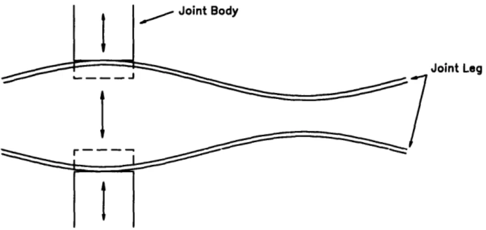
Structural joints play a critical role in the dynamic behavior of structures [3]. The vibrational energy present in a structure propagates along the individual members and interacts at the joints where the energy is scattered and/or dissipated. Scattering produces transmission and reflection as well as conversion to flexural, longitudinal and torsional waves. Transmission and reflection are a measure of the extent to which vibrational energy is isolated while the scattering behavior of a specific joint can be advantageous for converting a certain wave type into a different wave type which may be more sensitive to dissipation.

Vibration isolation can be achieved by trapping a wave within a member of the structure, however, damping mechanisms must be incorporated in the joint or in the member to achieve adequate dissipation. Of particular interest is the ability of a structure to minimize transmission of longitudinal waves. Longitudinal waves possess high phase speed and practical means to dissipate longitudinal waves are not easily achieved. By maximizing the extent to which longitudinal waves are reflected from a joint is it then possible to trap the longitudinal energy and prevent the energy from propagating through the structure and, ultimately, into an undesirable medium, for example, the volume external to the hull of a submarine.

Dissipation mechanisms are easily achieved for flexural waves. This is important since flexural waves are often most easily excited in structures and much of the energy content of all wave types is present in the form of flexural waves. A structure whose joints maximize reflection is most desirable since the vibrational energy will be trapped within the structure. When this cannot be achieved it is desirable that longitudinal-to-flexural conversion occur at the joint. This may produce reflection and transmission in the form of flexural energy where the performance of dissipative mechanisms can be maximized. This is especially important when those members, intended to dissipate vibrational energy, provide support for very noisy equipment.

(16)

1.1 Previous Research

The research conducted in support of this thesis involved three joints: two different spherical pinned-joints and one rigid joint. Considerable research has been conducted in regard to rigid joints. Most of the work has been conducted on two-dimensional, compliant and non-compliant, right-angled joints [4-9]. More generalized work on compliant and non-compliant two-dimensional joints which are not restricted to right-angles has recently been conducted by Guo [10].

Limited work has been conducted with regard to spherical joints. Space joint systems often use special connectors formed by spherical balls for attachment of the truss members. One type of spherical joint that has been developed by Wayne State University

[11, 12] is a hollow sphere containing a number of hollow spheres with the intent that the

spherical configuration forms a structurally rigid node. All spheres are in contact with one another and the spaces between the spheres may be filled with material to take advantage of its damping behavior.

Mathematical modeling and stochastic simulation of a three-dimensional spherical joint similar in design to that at Wayne State University has been investigated [13, 14]. Most published information on spherical joint behavior is, however, experimental and is

devoted to a specific joint configuration without generalization of the results. It has been observed [15] that much of the design knowledge for spherical joints is proprietary and is not published.

1.2 Objective

In order to facilitate proper design of the truss it is essential to understand the dynamic behavior of its structural joints since joint behavior plays a critical role in determining overall structural response to excitation. The objective of this thesis is to study the behavior of three simple, yet very different, laboratory-scale three-dimensional

(17)

joints through experimentation and application of analytical theory. Of primary interest is understanding the scattering of an incident longitudinal wave in each of the joints.

It is expected that the joints will behave significantly differently from one another and once this difference is recognized and understood it will be possible to utilize these characteristics to the greatest advantage. The pragmatic objective in understanding joint behavior is to be able to utilize favorable characteristics of specific joints to resolve specific vibration problems.

1.3 Approach

The three joints are designed such that the angular positions of the legs are identical to the simplest joint in the three-dimensional truss used in previous research in the MIT Acoustics and Vibration Laboratory [16]. In each experiment, each leg of each joint is connected to a 14' stainless steel leg extension to facilitate data collection. Impulse excitation is used to generate longitudinal incident waves. Accelerometers are placed on each leg to measure the acceleration from each wave type. Measurement of each wave type permits the determination of the transmission efficiency of each joint.

The intent is to gain an understanding of the scattering processes that occur when an incident longitudinal wave interacts with each joint. To this end, a scattering matrix is introduced which relates the input wave types to the output wave types. The elements of the scattering matrix are transfer functions which, in essence, are reflection and transmission functions of frequency. By experimentally determining the transfer functions it is possible to predict the output wave types for any given input; inherent in the use of the scattering matrix in the assumption of linearity. Comparison is then made to analytical two-dimensional work [4, 8, 10].

(18)

Chapter 2 Apparatus

The apparatus discussed in this chapter includes the descriptions of the joints,

experimental configuration, and the data acquisition equipment.

2.1 Joint Descriptions

Three joints were used in the laboratory experiments. Joint 'A' is a rigid joint

similar in construction to the joints used in the three-dimensional truss [16]. Joint 'B' is a

spherical pinned-joint with contact surfaces coated with Teflon. Behavior is intended to

be similar to a frictionless pinned-joint. Joint 'C' is very similar in design to Joint 'B' but

with the contact surface comprising visco-elastic material. The visco-elastic material is

discussed in Appendix C. Each joint has three legs, the simplest configuration used in the

three-dimensional truss. Design details of each joint are included in Appendices A, B, and

C for Joints 'A', 'B' and 'C', respectively. Figs. 2-1, 2-2, and 2-3 depict each joint as

used in the laboratory.

The joints are similar in size to those in the three-dimensional truss. Joint 'A' most

closely resembles the joint in the truss. The intent of the design of each joint was to

maximize simplicity without compromising practical application. Table 2.1 depicts the

mass of each joint. It should be noted that the mass of Joint 'A' has been corrected to

take into account the fact that its legs are longer than those of Joints 'B' and 'C'; the mass

of Joint 'A', presented in Table 2.1, is its effective mass.

Joints 'A', 'B', and 'C' are geometrically identical. Legs 1 and 3 intersect at 90

degrees. Leg 2 lies at 63.4 degrees to the plane formed by Legs 1 and 3; its normal

projection onto the plane formed by Legs 1 and 3 bisects the angle formed by Leg 1 and

Leg 3.

(19)

Table 2.1: Joint masses.

Joint 'A' (Rigid Joint).

'A' (Rigid) 588

'B' (Teflon) 997

'C' (Visco-Elastic) 979

(20)

Joint 'B' (Spherical Pinned-Joint, Teflon coated contact surfaces. Joint

'C' is identical at this scale.).

Joint 'B' (top section, bottom section, and spherical male leg). Figure 2-2:

(21)

2.2 Experimental Configuration

Figure 2-4 shows the laboratory experimental configuration. Each leg depicted in

Fig. 2-4 is 14 ft. long. Legs 2 and 3 are bare with no damping treatment while Leg 1 has

damping treatment. The intent of the damping treatment is to dissipate flexural energy

created by the longitudinal impulse such that a pure longitudinal wave is incident at the

joint.

Each joint is connected to the 14' legs by threaded connections. The tripod

configuration provides the support for each joint. Leg 1 is also supported by bungee cord

at the mid-section since the weight of the leg and the damping treatment is enough to

cause it to collapse.

Not depicted in Fig. 2-4 is a loading configuration which was applied during all

phases of experimentation. A force of 89 N was applied as shown in Figure 2-5. This

loading configuration ensured that each leg remained under an equal static compressive

load of 60 N. It also ensured that the spherical male legs of Joints 'B' and 'C' remained in

contact (under static conditions) with the joint body, thereby preventing an artificially high

impedance mismatch at the leg/joint body connection.

There is no theoretical basis for the selection of the value of the applied force. The

objective in selecting the magnitude of the force was: (1) the force would be great enough

to ensure that the spherical male legs remained in contact with the spherical recesses of the

joint body under static conditions and (2) the load would not cause the leg extensions to

buckle. The magnitude of the load does not ensure that the spherical male legs will remain

in contact with the surfaces of the recesses of the joint body during high levels of

excitation.

Coordinate System

A coordinate system is established for each leg. It is this coordinate system, shown in Fig. 2-6, to which reference is made in regard to flexural wave measurement. The y-axis is perpendicular to a given leg and has a component directed vertically

downward. The x-axis is horizontally directed.

(22)

C a 0 o c5 ! J

(23)

int

M1 &3

Figure 2-5: Static compressive loading configuration (cut-away side view of experimental model).

y-axis

Side View of Leg Leg Cross-Section

Figure 2-6: Coordinate system.

Leg 2

(24)

2.3 Data Acquisition Equipment

Vibrational excitation was achieved by using an instrumented impulse hammer.

The impulse hammer was a PCB Impulse Hammer with a plastic/vinyl tuning mass and an

aluminum extender. 8 Kistler 0.5 gm Type 8616A500 accelerometers were attached to

each leg to be able to differentiate between four different waves present in each leg, e.g.,

longitudinal, torsional, and two orthogonal flexural waves. The accelerometers have a

measuring range of ± 500 g and a transverse sensitivity of 5.0%. The low mass of the

accelerometers minimizes the added mass effect when mounted on a leg while providing

sufficient frequency range and sensitivity. Each accelerometer is attached with bee's wax

which provides a rigid connection to the leg over the frequency range of interest. Fig. 2-7

depicts the attachment of the accelerometers to a leg. Fig. 2-8 illustrates how each pair of

accelerometers are arranged to permit wave type determination. Appendix E provides

greater detail of exact accelerometer position and orientation.

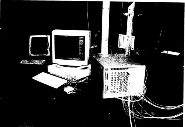
Fig. 2-9 shows the equipment used for data acquisition. This consisted of the

following:

(a) one HP 9000 Model 735/125 workstation

(b) one HP E1401A High-Power Mainframe

(c) six HP E1431A 25.6 kHz Eight Channel VXI Input Modules

The HP 9000 Model 735/125 is a high-performance PA-RISC-based workstation

that is designed to run the HP-UX operating system.

The six HP E1431A 25.6 kHz Eight Channel VXI Input Modules are installed in

the HP E1401A High-Power Mainframe forming a 48-channel data acquisition platform.

Each module is capable of sensing input frequencies ranging from 0.39 Hz to 25,600 Hz.

The sampling rate can be adjusted from 1 to 65536 samples per second providing a

minimum sampling interval of 1.52588 x10

-5

_{sec. The sampling interval throughout the}

(25)

The accelerometers are mounted onto the experimental model and are then connected by a thin coaxial cable to the HP E1431A Input Modules of the HP E1401A High-Power Mainframe.

The software used for data acquisition and post-processing was SDRC I-DEAS Master Series 2.0.

Figure 2-7:

Accelerometer configuration.

0 0

0

flexural

torsional

longitudinal

Figure 2-8: Orientation of an accelerometer pair in a typical cross-section to measure

wave types. Specific polarity for each leg is depicted in Appendix E.

flexural

(26)

(27)

Chapter 3 Experimental Execution

3.1 Impulse Excitation

Excitation for all phases of experimentation was conducted with an impulse generated by

an instrumented impulse hammer discussed in Chapter 2. The duration of each impulse was

typically 0.1 - 0.2 msec. Impulse excitation is the only viable means to ascertain joint dynamic behavior due to the limitations of the experimental model and the high phase speed of the longitudinal wave (approx. 5140 m/s). All joints were tested under two conditions: 1) an impulse to create a pure longitudinal wave, and 2) an impulse to create a pure flexural wave. Generation of a pure longitudinal incident wave was successful. Generation of a pure flexural incident wave was not successful; this is discussed fully in Appendix E. Each joint was tested with ten impulses for each of the two different types of impulses. The remainder of this thesis will focus on the incident longitudinal wave experiments.

3.2 Windowing

Time-gating the experimental data was necessary to prevent contamination. Contamination would come from reflection at the joint or reflection from the ends of the legs. As such, each leg was time-gated prior to the arrival of any reflected waves. The length of the window is solely dependent upon the speed of the longitudinal wave. The window established for Leg 1 was different than the window for Legs 2 and 3 as shown in Figs. 3-1 and 3-2.

The temporal windowing function applied in the windowing process is a flat filter of value

1.0 with ends tapered according to the function cos2 _t. _{The tapering is necessary to mitigate}

(28)

Leg 1 Windowing

Given that the length of each leg is 14', the propagation time for a longitudinal wave from the end of Leg 1 to the joint is 0.83 msec. This is the same time for the longitudinal wave to travel from the set of accelerometers to the joint and, after reflection, back to the accelerometers. To avoid contamination from reflection, the window for Leg 1 was selected to be 0.83 msec (54 data points) starting at 0.42 msec and ending at 1.25 msec after the pulse was initiated. Fig. 3-1 illustrates the temporal windowing function and a typical waveform before and after the use of the window for an incident longitudinal wave on Leg 1.

Leg2 Windowing

The propagation time for a longitudinal wave to travel from the end of Leg 1 to the group of accelerometers on Legs 2 or 3 is approximately 0.89 msec. Given that the distance from the group of accelerometers to the end of Legs 2 and 3 is 13', the propagation time for a longitudinal wave to travel from the group of accelerometers and back to the group, after reflection, is approximately 1.54 msec (99 data points). Hence, the window for Legs 2 and 3 was selected to be 1.54 msec wide starting at 0.89 msec and ending at 2.43 msec after the pulse was initiated. Fig. 3-2 illustrates the temporal windowing function and a typical waveform before and after the use of the window for a transmitted longitudinal wave on Leg 3.

Figure 3-1: Example of the windowing process for a typical incident longitudinal waveform (Leg 1).

C

5000

0 -5000

C

I I I I I I

50

2

1

0

(0

50

· 0

(31)

Chapter 4 Scattering Matrix

4.1 Principle

Conceptually, the dynamic behavior of each joint can be described by a matrix

whose elements are transfer functions. If a specific known wave type propagates along

one leg of the joint, it will be scattered at the joint and typically form, through

transmission and reflection, four different waves in each leg. These will comprise a

longitudinal wave, a torsional wave, and two orthogonal flexural waves. If, for example,

Leg 1 is excited by a pure longitudinal wave, that wave will propagate along the leg and

undergo scattering at the joint. Legs 2 and 3 will posses all waveforms that were

transmitted from the joint upon scattering. Leg 1 will not only be excited by the initial

wave type, it will also be excited by the reflection from the joint.

This matrix will be termed a 'scattering matrix'. The scattering matrix has the

form,

Z•1()

z

12

(f) Z

13

(f

z

14

()-Z2

1

() z7

2

2(n

z

3

(f)

ZM(00

3l(f)

Z3(f)

Z33Y) Z34f)

Z41(f) 20(f) z43(n Z4(f)_

where each element is an explicit function of frequency (Hz).

The scattering matrix may be used to determine the resulting output waveforms of

each leg by post-multiplying by the input function The input function takes the form of a

4x1 matrix where

s,

(f) may, for example, be the input longitudinal wave:

(32)

The resulting output from the scattering process has the form:

y1,f)

ZII,)

z1(2)

Z13)

z314 )

.yO4)_ _,,q'

z,,•)

z41f) z.(f)J

Y3 W

ý31

Z32

b~

Z53f Z134 WJ

2s

3

()I

4.2 Joint Scattering Matrices

Associated with each joint are three scattering matrices, one scattering matrix for

each leg. The scattering matrices determine the wave types that will be present in a

specific leg for a given input. Joints 'A', 'B', and 'C' thus require the determination of 9

unique matrices to describe their dynamic behavior. All Leg 1 matrices contain elements

which are reflection functions. All Leg 2 and Leg 3 matrices contain elements which are

transmission functions.

The first column of each matrix contains the functions which are the response due

to flexural excitation in the y-direction. The second column contains the functions which

are the response due to flexural excitation in the x-direction. The third column contains

the functions which are the response due to torsional excitation. Lastly, the fourth column

contains the functions which are the response due to longitudinal excitation.

(33)

4.2.1 Joint 'A' Scattering Matrices

The three scattering matrices associated with Joint 'A' are formally defined below for further reference.

Joint 'A' Leg 1 Scattering Matrix:

all(f) a12(f) a13(f) a14(f)

21Y)

22Y)

a

3(0

a

-

41 42

23 2440

allP a32•) a33()

a34(P

_a4l(f,

a4:•) a4•(f af_

bf)

b14

2

()

b

13

(f) b14

(f)

bzl(f)

b22

f)

b23(f) b

24

(f)

b

31

()

b

32

(f) b

33

(f) b34(f)

b4,

Yt

be42

b43(

b44tr

c,,(f)

c

12

(f) c

3

()

c

14

(f)]

C

21

(f) c

22

(f) C

23

(f)

24

(f)

C

31

(f) C

32

(f) c

33

(f)

C

34

(f)

I

(34)

4.2.2 Joint 'B' Scattering Matrices

The three scattering matrices associated with Joint 'B' are formally defined below

for further reference.

Joint 'B' Leg 1 Scattering Matrix:

4

1 (t)

d

21

(f)

d3

₁

₀

-d

41

()

d~

2

(f)

d12

d22Y)

₃₃

_(f)

d

₄₃

(f)

d

14

(f)

d4

f)

d,(f)

d44

()

Joint 'B' Leg 2 Scattering Matrix:

e

11

,,(f)

e

21

31

(f)

-e

41

(f)

e

22

e

32

(f)

e

42

(f)

_(f)

44 -Joint 'B' Leg 3 Scattering Matrix:

A

1 f2A

1 A

1 141

0f

(f)

0f

A

2

(f)

f

2

(

0 A

2

f

42

0 f23 (n

A

3 f33

Asm f

f4W

A4 (

A4W

f

44 (f)

(35)

4.2.3 Joint 'C' Scattering Matrices

The three scattering matrices associated with Joint 'C' are formally defined below

for further reference.

Y)

14

(f)

g

24

(f)

g

34

(f)

94

-Joint 'C' Leg 2 Scattering Matrix:

h24

_h4i"o

/z

12 (f)

k

12

(f)

/

22

(f)

k

₃₂

_(f)

k42

(t

k

13

(f)

k

33

(f)

'(f)

k43(n

k.(f)n

(36)

4.3 Determination of Joint Scattering Matrices

As discussed previously, output wave types can be determined by post-multiplying a specific scattering matrix by the input function. Experimentally, however, the objective is to determine the scattering matrix from the given input and resulting output. The elements of the scattering matrix are most easily determined by injecting pure waves of one type into the joint. This permits determination of the elemental transfer function directly from known input and known output.

If, for example, a pure torsional wave is injected into Leg 1 of a joint, Leg 1 will

experience reflection and all four waves (longitudinal, torsional, and two orthogonal flexural waves) will, typically, be present. Similarly, each of Legs 2 and 3 will, typically, be excited by four transmitted waves.

The problem of determining the elemental transfer functions is much more difficult if more than one wave type is simultaneously injected into the leg. By injecting pure waves into a leg the scattering matrix can be simplified and the elemental transfer functions can be readily determined. Let the input matrix be specified as

[F, ()

F(

T, (

L, (n

,

where F,, (f) is the flexural wave in the y-direction, F, (f) is the flexural wave in the x-direction, T, (f) is the torsional wave, and L, (f) is the longitudinal wave. If a pure flexural wave in the y-direction is injected into Joint 'A', the input matrix simplifies to:

(37)

The resulting scattering equation for Leg 1 of Joint 'A' becomes:

Fyr

a,

I 1

Fvr(f)1

ra

a(f)

Tr,

(f)

a (f)

L()

I(

La

A

4)

[i;;

_f)]

The elemental transfer functions for the pure input flexural wave (in the y-direction) are

thus readily determined to be:

F, (f) F (f)

a, (f) =

Fy(f)

a

1 2

(f)

=

F

(f

a

13

(f) =

al4(f

=

(

F,, (

f

) "

F,, (f )"

By injecting a pure wave of each type into Leg 1 it is possible to determine the

elemental transfer functions for each of the three matrices of Joints 'A', 'B', and 'C'; this

method computes the columns of each scattering matrix. In principle, the determination of

the elemental transfer functions for each matrix is straight forward. In practice, it is not

easily achieved.

4.3.1 Transmission Function Derivation Using the Concept of Reciprocity

Describing the dynamic response of a structure to a given excitation is a very

difficult problem. Consideration is made of the simple case where a structure is excited by

a single force component at one location and the response velocity is measured at another

location. By using transfer mobility it is possible to relate the force at one location to the

response velocity at another location. It is also possible to demonstrate that the transfer

(38)

M-mobility is reciprocal [5]. Namely, the ratio of the excitation force at some location 'a' to the response velocity at location 'b' is equal to the ratio of the force measured at location 'b' and the velocity at location 'a'.

Reciprocity is only valid if three basic requirements are satisfied:

1. The system should be passive; no sources other than those used for excitation should exist.

2. The system should be linear; the response should be at the same frequency as the excitation and proportional to it.

3. The system should be bilateral. When the phase or direction of the excitation is altered the response should change in a likewise manner.

Reciprocity can also be viewed as: the ratio of the power in a transmitted flexural wave to that in an incident longitudinal wave equaling the ratio of the power in a transmitted longitudinal wave to that in an incident flexural wave [4]. Namely,

PP

- . (4. 1)

As an example, acceleration for an input longitudinal wave takes the following form

oF,/

o,,c/F

a, = ovli•

Z

(4.2)

Likewise, acceleration for an output flexural wave takes the following form

a-

o - Of (4.3)

ao

/ou Z=o_, _pcf

The transmission function for each joint is defined as the ratio of the output acceleration of a specific wave type to the input acceleration of a specific wave type. For the case where the excitation wave type is longitudinal and the output wave type is flexural the

(39)

transmission function, Tr, is defined as

afout _{Ff outC}

i = - = (4.4)

al,, Fl ,, cf

Using reciprocity it is then possible to determine the transmission function, T2, for a given input flexural wave and a resulting longitudinal wave

alou_t Fl out C _f

2

=

F-

c

(4.5)

a

_1.

_{Ff ,C}

It is this tool, reciprocity, which permits additional elemental transmission functions of the scattering matrices to be determined.

Expanding (4.1) results in

Sa

-

(4.6)

F a F a

for a harmonic response.

Substitution of -, and -2 into (4.6) yields

Ff 2 F2 Cf 2

F = -

Ff,2

C (4.7)

F/2 _F 2

1,

and simplification results in

ciFf,, _Fl.•

I .

F _(4.8)

cf Fl F,

The left-hand side of (4.8) is, by definition, r, and multiplying both sides of (4.8) by the ratio of flexural phase speed to longitudinal phase speed results in

(40)

cf Fr c

r1 - (4.9)

c, F,, cI

The right-hand side of (4.9) is, by definition, r2 and further manipulation of (4.9) results in the reciprocal relation between r, and r2,1

C

2 -= &f. (4.10)

Cl

Alternatively, (4.10) may be written as

r2 = I - , (4.11)

where cf = 1KCC .

Similarly, for the case in which the reciprocal transmission function is desired for the case in which a torsional waveform is present, the relation becomes

CT2

1 (4.12)

(41)

Chapter

5 Analytical Models and Predictions

5.1 Transmission from Flexural Wave Excitation

Wave transmission through right-angled structural joints has been studied

previously [3

-

9]. Guo developed a generalized analytical formulation [10] focusing on

flexural wave transmission through structural joints without the restriction to a

right-angle. This analysis is two-dimensional and is based on a joint with two elastic beams

joined at an angle 0 depicted in Fig. 5-1. The joint is illustrated in Fig. 5-2 and is

modeled with stiffness, dissipation, and mass, in three degrees of freedom.

Structural Joint

1

ncidence

(42)

Figure 5-2: Model of two-dimensional joint with stiffness, dissipation and mass.

This model assumes incident flexural waves are produced at a distance far away from the joint so that the evanescent field from incident bending motion can be neglected. In studying wave-joint interactions the energy carried by the different wave types is used to measure reflection, transmission, dissipation, and conversion. For this case of harmonic waves, the energy is measured by the power flow of flexural and longitudinal displacements.

In this model, incident waves may cause motion at the joint in three degrees of freedom: longitudinal displacement, transverse displacement, and rotation. Spring-dashpots are used in all degrees of freedom so that the effects of joint constraints on motion can be studied independently. The springs are assumed to have complex spring constants such that the real part specifies the spring stiffness and the imaginary part specifies the loss factor. Through the use of complex spring impedances, the forces acting on the joint include both spring forces and dissipative forces. Similarly, the moments are given by the rotation of the joint through the use of a complex spring constant in rotation. The equations of motion of the joint are determined to be

(43)

m2mX = sin(O / 2)(fL - fLA2)+ cos( / 2)(fF, + fF2), (5.1)

w2m Y = cos(O / 2)(fL2 fLl))+ sin(O / 2)(fFr + fF2), (5.2)

COm2

= (M2, -_

M)

2

.

(5.3)

The motion of the joint can then be specified by balancing all forces and moments acting on the joint, these forces and moments being identical to those acting on the two connecting beams at the point where the two meet. The forces acting on the joint are

fL1 = z, [Y cos(O / 2) + X sin(O / 2) - u], (5.4)

fL2

= _{ZL[Y COS( / 2) - X sin(O / 2) + u}

2] , (5.5)

fF1 = F[Y sin(O / 2)- X cos(O / 2)- w- w], (5.6)

fF2 = zF[Y sin(O / 2) + X cos(O / 2) - w₂] . (5.7)

Similarly, the moments are given by the rotation of the joint, (D, and rotation present at the ends of the two beams, w, and w2,

M, = zm,(wl -

D)

and M

2

= zM(D-

w).

(5.8)

By substituting (5.4) through (5.8) into (5.1) through (5.3) the displacements and

rotation may be determined as

Sz, sin(O / 2)(u, + u2)- zF Cos(O / 2)(w, - w2) (5.9) 2zL sin2(0 / 2)+ 2zF Cos2(6/ 2)_ w2m

= zL cos(O / 2)(u, - u2)+ z, sin(O / 2)(w, +w2)

2L cos2_{(012)+ 2z sin}2_(/2)- 2_m _(5.10)

zM,(w +w,

z= ( 2 2 _(5.11)

2_Zy

(44)

By setting M to zero and setting all joint stiffnesses to infinity it is possible to

derive the efficiency of transmission for the rigid joint.

For rigid joints without mass [10], the flexural-to-longitudinal transmission

function (ratio of output acceleration to input acceleration) is

[2(i + ) + (ip + 1)(1- cos )]

TL =-2sin

_{u(1 +}

_i)(2cos

_{0 -}

₃

_{- 3cos}2 _{0) 2(p2 +i) sin}

(5.12)

where p = f C1

Since no analytical solutions exist for the three-dimensional joint, comparison will be made between the two-dimensional analytical model and the three-dimensional physical model. For an incident flexural wave on Leg 1 and a transmitted longitudinal wave on Leg 3 (0 = 900), (5.12) reduces to

(2i+ 2,u + iu + 1)

TL'2P, 2 lp . (5.13)

(3p + 3iu + 2,U 2 + 2i)

Similarly, for an incident flexural wave on Leg 1 and a transmitted longitudinal wave on Leg 2 (0 = 71.50), (5.12) reduces to

3.8i + 3.8" 2 + 1.298u2i + 1.298 p

T = (5.14)

2.667 p + 2.667 pi + 1.8 2 + 1.8i

5.2 Transmission from Longitudinal Wave Excitation

Longitudinal wave propagation through right-angled joints has been analyzed by

Leung and Pinnington [8]. The analytical solutions for the rigid joint approach that

presented by Cremer [4]. This model assumes an incident longitudinal wave of the form

(45)

xl vxl+ (e- j_kx _{+ rLe+jx).}

(5.15)

The transmitted waves take the form of

v = vxl+ (te - J Y _{+ tje}

(5.16)

vy2 =

Vxl+tLLe

y

_(5.17)

These equations are then substituted into the boundary conditions. The boundary conditions consist of matching moments and rotational velocity on both sides of the joint. The final boundary condition which must be applied consists of matching shear forces. The incident longitudinal shear force will create a bending wave in the second leg and this force is equal to the bending shear force in the second leg. The incident longitudinal force has no effect on the longitudinal wave in the second leg.

It is from these boundary conditions that the transmission efficiencies are derived. In the case of a rigid joint for which the x-direction, y-direction, and rotational impedances are infinite, the flexural transmission function (ratio of output acceleration to input acceleration) for an incident longitudinal wave [4] is expressed as

5p2 +8p 2

rF 2+-

+

2

(5.18)

2+6p +9P2

Similarly, the longitudinal transmission function (ratio of output acceleration to input acceleration) for an incident longitudinal wave can be expressed as