DUST IN THE CIRCUMGALACTIC
MEDIUM OF LOW-REDSHIFT GALAXIES
The MIT Faculty has made this article openly available.
Please share
how this access benefits you. Your story matters.
Citation
Peek, J. E. G., Brice Menard, and Lia Corrales. “DUST IN THE
CIRCUMGALACTIC MEDIUM OF LOW-REDSHIFT GALAXIES.”
The Astrophysical Journal 813, no. 1 (October 21, 2015): 7.
doi:10.1088/0004-637x/813/1/7. © 2015 The American Astronomical
Society
As Published
http://dx.doi.org/10.1088/0004-637x/813/1/7
Publisher
IOP Publishing
Version
Final published version
Citable link
http://hdl.handle.net/1721.1/100756
Terms of Use
Article is made available in accordance with the publisher's
policy and may be subject to US copyright law. Please refer to the
publisher's site for terms of use.
DUST IN THE CIRCUMGALACTIC MEDIUM OF LOW-REDSHIFT GALAXIES
J. E. G. Peek1,2, Brice Ménard3,4,6, and Lia Corrales2,5 1
Space Telescope Science Institute, 3700 San Martin Dr., Baltimore, MD 21218, USA;jegpeek@stsci.edu
2
Department of Astronomy, Columbia University, New York, NY, USA
3
Department of Physics & Astronomy, Johns Hopkins University, 3400 N. Charles Street, Baltimore, MD 21218, USA
4
Institute for the Physics and Mathematics of the Universe, Tokyo University, Kashiwa 277-8583, Japan
5
MIT Kavli Institute, 77 Massachusetts Ave. 37-241, Cambridge, MA 02139, USA Received 2014 May 9; accepted 2015 September 16; published 2015 October 21
ABSTRACT
Using spectroscopically selected galaxies from the Sloan Digital Sky Survey we present a detection of reddening effects from the circumgalactic medium of galaxies which we attribute to an extended distribution of dust. We detect the mean change in the colors of“standard crayons” correlated with the presence of foreground galaxies at
z~0.05as a function of angular separation. Following Peek & Graves, we create standard crayons using passively evolving galaxies corrected for Milky Way reddening and color-redshift trends, leading to a sample with as little as 2% scatter in color. We devise methods to ameliorate possible systematic effects related to the estimation of colors, and wefind an excess reddening induced by foreground galaxies at a level ranging from 10 to 0.5 mmag on scales ranging from 30 kpc to 1 Mpc. We attribute this effect to a large-scale distribution of dust around galaxies similar to thefindings of Ménard et al. We find that circumgalactic reddening is a weak function of stellar mass over the range6 ´109M
–6 ´1010M and note that this behavior appears to be consistent with recent results on the
distribution of metals in the gas phase. We alsofind that circumgalactic reddening has no detectable dependence on the specific star formation rate of the host galaxy.
Key words: dust, extinction– galaxies: evolution – galaxies: formation – galaxies: halos
1. INTRODUCTION
Galaxies process and return a significant fraction of their accreted gas to their surroundings, the circumgalactic medium (CGM), but the physical mechanisms involved as well as the matter distribution in this environment are still poorly constrained. Much of our knowledge of the distribution of baryons in the CGM comes from absorption line studies which probe the gas phase. The interpretation of such measurements is often limited by our lack of knowledge of the ionization state of the gas. In this work we explore the distribution of dust around galaxies and use it as an alternative tracer of metals in this environment, independent of ionization corrections. It is important to realize that a substantial fraction of CGM metals might be in the solid phase. In the ISM, about 25% of the metals are found in dust (Weingartner & Draine 2001). Measuring dust reddening effects from the CGM may also allow us to put constraints on the grain size distribution and potentially the mechanisms responsible for their ejection from galactic disks to halos, for example, supernova explosions(Silk 1997; Efstathiou 2000) or radiation pressure (e.g., Murray et al.2005; Salem et al.2014).
A number of authors have reported the presence of dust well beyond galaxy disks. Using superpositions of foreground/ background galaxies, Holwerda et al. (2009) detected dust extinction up to about five times the optical extent of spiral galaxies. Using deep Herschel observations, Roussel et al. (2010) showed that emission from cold dust is seen up to 20 kpc from the center of M82. Using UV light scattered by dust grains, Hodges-Kluck & Bregman (2014) reported the detection of dust up to about 20 kpc perpendicular to the disk of edge-on galaxies. With a statistical approach, Ménard et al. (2010, MSFR) measured the cross-correlation between the
colors of distant quasars and foreground galaxies as a function of the impact parameter to galaxies. They found an excess reddening signal on scales ranging from 20 kpc to a few Mpc, implying that the distribution of dust extends all the way to the intergalactic medium. Ménard & Fukugita(2012) showed that a similar amount of dust can been seen associated with strong MgII absorbers at 0.5 < z < 2.0, providing another line of
evidence of the presence of dust on large scales around galaxies. Fukugita (2011) showed that the summed contribu-tions of dust in and outside galaxies appears to be in agreement with the total amount of dust that ought to be produced in the universe. This implies that dust destruction does not play a major role in the global dust distribution and that most of the intergalactic dust survives over cosmic time.
In this work we focus on the low-redshift universe and constrain both the amount of dust surrounding nearby (z ∼ 0.05) galaxies and its dependence on galaxy properties. We do so by using a set of standard crayons, following the work of Peek & Graves(2010,PG10), i.e., galaxies for which the colors can be standardized. The outline of the paper is as follows. In Section 2 we describe the data sets and how we estimate the color of a standard crayon galaxy. In Section 3 we introduce our estimator for reddening measurement. In Section 4 we present our analysis and results showing both detections of reddening and the variation of this reddening as a function of foreground galaxy parameters. We discuss these results in the context of galaxy formation and metal budgets in Section5, and conclude in Section6.
2. DATA
Our goal is to measure the mean color change of distant sources induced by the presence of foreground galaxies, as a function of impact parameter, R. Optimizing such a measure-ment requires both maximizing the number of
foreground-The Astrophysical Journal, 813:7 (9pp), 2015 November 1 doi:10.1088/0004-637X/813/1/7
© 2015. The American Astronomical Society. All rights reserved.
6
background pairs and minimizing the possible scatter in the color distribution of the background objects. To do so we work with data drawn from the Sloan Digital Sky Survey (SDSS; York et al. 2000).
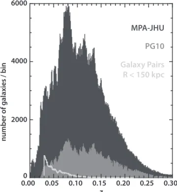
For our foreground population we select galaxies from the Main Galaxy Sample from data release 7(Strauss et al.2002) and use the magnitude limited selection r < 17.77. This produces a sample of 695,652 foreground galaxies for which two intrinsic properties are extracted from the MPA-JHU value-added catalog (Kauffmann et al. 2003; Brinchmann et al.2004): specific star formation rate (sSFR) and stellar mass (M). The distribution of galaxies as a function of redshift is
shown in Figure1 with the black histogram.
For our background sample we make use of standard crayons, as introduced by PG10: objects whose colors have a very narrow distribution. We select passively evolving galaxies from the Main Galaxy Sample (again, r < 17.77) using the criterion that they have neither detectable OIInor Hα emission,
as measured by the NYU Value Added Catalog (Blanton et al.2005), significantly limiting their number. Their colors are then adjusted for the color–magnitude relation as a function of redshift, a procedure described in more detail below. As a result, their Galactic reddening-corrected colors have an extremely narrow distribution. The details of that selection procedure are discussed in PG10. This provides us with a sample of 151,637 galaxies. We note that we do not exclude these galaxies from our foreground sample described above. The redshift distribution of the background galaxies is shown in Figure1 in gray.
To estimate color changes we use the apparent model magnitudes of the galaxies and apply two corrections to them.
First, we correct for the effects of Galactic dust reddening. To estimate them we avoid using the standard dust map from Schlegel et al.(1998) which relies on FIR emission, known to originate not only from the Milky Way but also from low redshift galaxies(see Yahata et al.2007; Kashiwagi et al.2013; Peek & Schiminovich 2013, for a discussion of the effect). Instead, we emulate the work of Burstein & Heiles (1982) and estimate extinction with a neutral hydrogen column, as measured by the Leiden–Argentina–Bonn radio survey (Kalberla et al. 2005). This is a commonly used method for determining extinction toward a source with significant FIR emission, for example, nearby galaxies (e.g., Cordiner et al. 2011). We define the Galactic dust reddening DMW, measured in the bands a and b, in a given direction in the sky by C R R N 7 10 cm , 1 a b MW H 21 2 I
(
)
( ) D = -´-where Raand Rbare the Galactic extinction coefficients for the SDSS bandpassfilters (Stoughton et al.2002), and the ratio of reddening to HI for this region is derived from Peek (2013),
Equation (2). We exclude galaxies with a measured
E B( -V)>0.1, where the HI column is known to be a
poor reddening estimate, removing 1891 galaxies from our background sample. We note that using the Schlegel et al. (1998) extinction rather than the method described above changes all values quoted in this text by less than 10% and by less than 10% of their quoted errors. We further note that any zero-point offset between Schlegel et al. (1998) and HI
methods is absorbed by the fact that we are only concerned with deviations from the average color of the sample. Second, we need to remove possible trends between background galaxy colors and redshifts, which stem both from galaxy evolution and “K-correction.” To do so we measure the median color-redshift relation for each of the 10 SDSS optical colors and characterize it using a fourth-order polynomialfit, refered to as
Credshift.
D We show thesefits for four colors in Figure2. With these two correction terms in hand wefinally define the corrected color of a background galaxy by
Ccorr=Cobs- DCMW- DCredshift. ( )2 This provides us with a distribution of corrected colors Ccorrfor
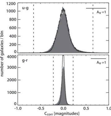
which the dispersion ranges from 21(r − i) to 180 mmag (u − z) depending on the chosen bands. Figure 3 shows examples of these color distributions alongside the color distributions presented in PG10. The distributions in PG10 are slightly narrower because additional regressions(color–magnitude and color–density relations) were applied in that work.
2.1. Outlier Rejection
To increase the robustness of our statistical analysis wefirst remove outliers in the color distribution of the background galaxies(PG10, Figures 2 and 3). To do so we use Chauvenet’s criterion, rejecting outliers that have larger deviations in color than would be expected (given a sample size and standard deviation). We reject galaxies that fail to meet this criterion in any of the 10 colors, which removes 7861 galaxies from the sample, i.e., about 5% of the data. We note that arbitrarily moving the threshold such that we reject half or twice the number of galaxies, or simply clipping at 3σ does not effect our
Figure 1. Redshift distribution of the selected galaxies. The dark histogram represents all the foreground galaxies from the Main Galaxy Sample of SDSS DR7. The background quiescent galaxies fromPG10are shown in gray. The lightest colored unfilled histogram shows a distribution of the foreground galaxies that have at least one background galaxy within 150 kpc impact parameter.
reported results: the reported dust masses in Section 4.1and trends in Section 4.2are insensitve to these choices. We also test against a bootstrap analysis and do not detect differences in the measured errors. We conclude that the method by which we reject our outliers, sophisticated or simple, does not effect our results. Our extreme outlier rejection criterion is indicated as vertical dashed lines in the right panel of Figure 3. The final sample contains 141,885 background galaxies.
3. METHODS
Given that the expected level of CGM dust reddening is lower than the intrinsic width of the corrected color distribu-tion, we constrain its amplitude by measuring the mean color excess induced by the presence of foreground galaxies in a range of impact parameters, áC R( min,Rmax)ñ We chose.
different ranges of Rmin and Rmax, depending on the scientific questions explored in Section4.
In addition to reddening by dust, apparent color changes can stem from other effects and systematic errors: physical interactions between foreground and background objects (in galaxy groups and clusters) and/or distortions in the photo-metry due to the presence of a nearby galaxy and wide-field photometric errors. Below we define an estimator that takes those effects into account.
One requirement we put on our estimator is that it should not lead to any reddening signal if we measure the color changes of foreground galaxies as a function of angular separation from background galaxies. Any such change would indicate our estimator is sensitive to some non-physical effect, as light coming from a galaxy in front should not be modified physically by a galaxy behind. We refer to this measurement as the“reverse test.”
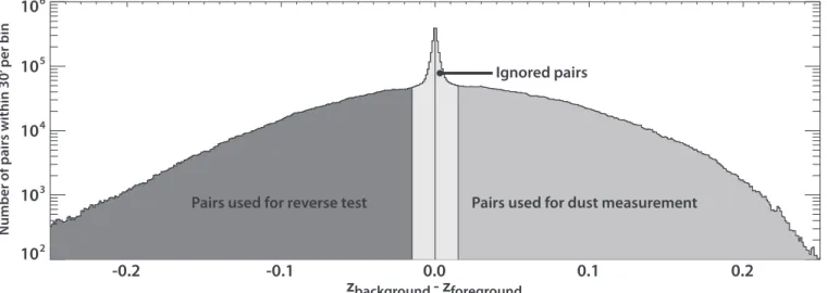
3.1. Physical and Lensing-induced Correlations Galaxies are known to follow a color–density relation (e.g., Blanton et al.2005) leading to mean color change as a function angular separation. To avoid being contaminated by such an effect, we impose a minimum redshift difference between our background and foreground objects. In Figure4 we show the distribution of foreground-background pairs within 30 arcmin as a function of zd =zbackground-zforegroundfor both the direct
reddening measurement (right) and the reverse test (left; see Section3.3). There is a sharp increase in the number of pairs on small scales, due to the clustering of galaxies. Guided by the visually evident clustering at∣dz∣ < 0.01seen in Figure 4, we conservatively ignore galaxy pairs with∣d <z∣ 0.015 (the light gray band). Changing this value by a factor of two does not change our results.
Gravitational lensing increases the brightness of background galaxies behind foreground galaxies. Because of this bright-ening, there will tend to be more background galaxies brighter than a given threshold in the vicinity of foreground galaxies (Narayan1989). The strength of this effect depends on both the gravitational magnification of the foreground population and the shape of the brightness distribution of the background sources. While our results are insensitive to background galaxy brightness, the average color of a population of galaxies will slightly change if the limiting magnitude is effectively altered. This effect, similar to the population reddening effect discussed
Figure 2. Distributions of background galaxy colors with redshift. The solid black line represents a fit to the median of the data, which we subtract to measure residual colors independent of galaxy evolution and“K-correction.”
Figure 3. Color distributions of background PG10galaxies. Histograms of originalPG10colors(black), and C ,corr (Equation (2); gray, filled), are shown
for u− g (top) and g − r (bottom) colors. The expected reddening for Milky Way dust with an Avof 1, Rv= 3.1 is shown by the black bar. The truncation
in Peek & Schiminovich(2013), is very small; for our sample less than 20 mmag of color changes per magnitude of bright-ening for all the colors we investigate. On scales of 150 kpc (about three arcminutes at the redshifts of interest), typical changes in galaxy brightness are ∼3 × 10⁻³ and drop with scale roughly as R−1 (Scranton 2005, MSFR). We therefore expect lensing-induced color changes to be∼ 5 × 10⁻⁵mag at R∼ 150 kpc. This term is insignificant and we neglect it in the following.
3.2. Wide-field Photometric Errors
We expect wide-field variations in the photometry and colors at some level, as the SDSS survey was conducted over varying conditions over many years. This can be induced by calibration offsets (Padmanabhan et al. 2008) or biases in the dust map (e.g., Peek 2013). These errors can exceed 40 mmag in some regions(PG10). Such large-scale variations may bias the color change we wish to measure: large scale structure in our foreground galaxies may overlap with regions of photometric error, generating a bias beyond simple Poisson noise. In order to mitigate this effect, we only focus on the excess color change measured with respect to a large-scale averaged mean color:
C R R C R R C
, ,
1 Mpc, 2 Mpc . 3
min max corr min max corr
( ) ( )
( ) ( )
D = á ñ
-We measure this effect to be typically of order 2× 10⁻⁴mag, and always smaller than our error bars and signal. We choose to use galaxies with an impact parameter between 1 and 2 Mpc as our“zero point” because we are chiefly interested in the dust in the CGM of galaxies, defined to be within the virial radius, which is always less than 1 Mpc. We note that this method restricts us to measuring dust with R< 1 Mpc and represents an imperfect mitigation of this very small effect.
3.3. Small-scale Photometric Biases
On small scales, photometric estimation can be affected by the presence of nearby extended sources, like bright galaxies (Aihara et al. 2011). The foreground galaxy is not a point
source, and thus may have a real extended light distribution. The fact that the background object is also a galaxy introduces additional opportunities for error. To consistently measure the apparent magnitude of a galaxy, one must fit a model to the galaxy profile, which requires a careful estimate of the sky brightness nearby. Any other galaxies in the same region of sky can bias the sky brightness estimate. Additionally, because we are examining pairs of galaxies, there is an opportunity for blending, where the SDSS photometric pipeline must disen-tangle the light from the foreground and background galaxy. In practice this happens less than 10% of the time for very close pairs(first radial bin discussed in Section4), and not at all for pairs with larger impact parameters.
Quantifying such effects as a function of galaxy proximity and brightness requires tests of the SDSS photometric pipeline (see Huff & Graves2013and future work discussed therein). Instead of attempting to predict the amplitude of these effects, we can directly estimate them using the reverse test introduced above, i.e., measuring the color changes of foreground galaxies as a function of angular separation from background galaxies. Such a correlation should not lead to any signal. Therefore any measured quantity is an estimate of the amplitude of photometric biases. We perform a photometrically and angularly matched measurementDCreverse.We weight galaxy pairs in the reverse test such that their pair-wise angular distribution matches that of the forward measurement. Ourfinal circumgalactic dust reddening estimator is thus
Cdust C Creverse. ( )4
D = D - D
This small-scale photometric bias is expected to depend on the brightness of the foreground galaxies. Since the reverse test will tend to have higher redshift “foregrounds” than the dust measurement, we also need to take this difference into account. We estimate DCreverse as a function of the magnitude of
“foreground” galaxies by binning the sample by quartiles in r band magnitude. Wefind that, in practice, the strength of this small scale photometric bias is insensitive to whether we bin by quartiles or in some other way, and whether we use r or another
Figure 4. Distribution of redshift differences for the galaxy pairs selected within 30 arcmin. The light gray region shows pairs used for the direct dust reddening measurements. The dark gray region shows pairs used for the“reverse test” used to characterize the effects of photometric bias, where the “background” galaxy is in front of the“foreground” galaxy. The lightest gray area at the center represents pairs that are likely to be related in physical space ( z∣ background-zforeground∣<0.015) and are thus not used in either measurement.
filter. A comparison of DCdust and DC is shown in the
following section.
3.4. Statistical Methods
Much of this work can be approached with standard statistical methods, where classical estimators for the mean and errors on the mean(c2) are appropriate. We are, however,
also interested in estimating the ratio of reddenings between two independent measurements, for instance the ratio of the reddening observed around large galaxies to the reddening observed around small galaxies. In this case we assume a priori that the true underlying reddening for a set of color measurements X is some ratio ρ times the true reddening a set of color measurements Y. The covariances matrices associated with the X and Y measurements are S andX SY. We assume zero covariance between X and Y, as the data are independent. Applying Fieller’s Theorem (Fieller1954) to this restricted case we find V I X Y I I , 5 T T X 2 Y
(
)
( ) ( ) r r = -S + Swhere I is simply a vector of ones representing a naive weighting. Here V is the statistical score:ρ where V = 0 is our point estimator of the ratio, and the range ofρ that corresponds to V = -[ 1, 1]is our 1-σ confidence interval.
4. RESULTS 4.1. Mean Reddening Signal
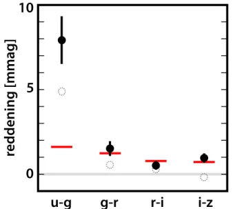
Using the color excess estimator presented in Equation(4) we measure the mean color excess induced by foreground galaxies as a function of impact parameter, from 30 to 750 kpc. In Figure5 we show the radial profile of the color excess for four radial bins. We detect a color excess signal of about 8(u − g), 2 (g − r), 1 (r − i), and 1 (i − z) milli-magnitudes at
Rp<150 kpc, which drops by an order of magnitude for
Rp>150 kpc.We attribute this signal to the presence of dust in the CGM and IGM. For comparison we show as dotted lines the best fit power-law trend to the results obtained by MSFR using foreground galaxies at z∼ 0.3 and background quasars to measure colors. Our measurement shows some differences with respect to the MSFR bestfit trend in both the steepness of the falloff beyond 150 kpc and in the much stronger color excess in u− g.
In order to investigate the extinction curve for CGM dust, Figure 6 plots the wavelength dependence of the measured color change in the region 30<Rp <150kpc, where the signal-to-noise ratio of our measurements is higher. The u− g color shows a significant excess, which is inconsistent with that of an SMC bar exctinction curve (red dashes, Weingartner & Draine 2001) at the shortest wavelengths. Fitting the data points in Figure 6 with an SMC extinction curve yields a reducedc of 7.6. We note that our u-band extinction is not2
affected by the canonical 2175Å (NUV) absorption “bump” at the redshift of our foreground galaxies, i.e., 0.03< z < 0.1.
In general, small dust grains contribute to a steeper slope on the blue end of an extinction curve, which might account for the excess in u− g reddening. To test the hypothesis that the increase in u− g color relative to SMC extinction (Figure6) is driven by the dust grain size distribution, we examine the very simplified case in which the dust has a single grain size and
Figure 5. Mean reddening excess measured as a function of scale, indicating the presence of a reddening agent in the CGM and IGM. Four bins are shown for each of four colors. The dotted lines shows the bestfit power law obtained by MSFR who measured the color excess induced by z= 0.3 galaxies on background quasars. Data points below 0.1 mmag (not shown) are all consistent with zero, but inconistent with the MSFR dotted line by the number of standard deviations indicated on the bottom of the figure. Our analysis indicates a steeper falloff with impact parameter than MSFR, and stronger u− g color excess.
Figure 6. Average reddening of background galaxies with impact parameters between 30 and 150 kpc of all spectroscopic foreground galaxies. Solid black circles represent our dust reddening estimatorDCdust(30 kpc, 150 kpc .) An excess reddening is detected in all color combinations. The red lines represent the results of MSFR, assuming SMC dust. For reference, the empty gray circles show the results without the reverse test debiasing,
C 30 kpc, 150 kpc ,( )
D the distace between the filled and empty circles is thereforeDCreverse(30 kpc, 150 kpc).
material. We do not expect that CGM grains are truly uniform, but we use this toy model as a simple test appropriate for our broadband data.
We investigate two extremely simplified dust models: graphite only and silicate only, each with a single variable grain size a. We use dielectric constants given by Draine (2003), Draine & Lee (1984), and Laor & Draine (1993) and compute Mie scattering and extinction cross-sections using the publicly availablebhmie code (Bohren & Huffman1983). We use these cross-sections to compute extinction curves, the slopes of which yield predictions for u− g, g − r, and so on (Figure 6). The best fit graphite and silicate models are
ag =0.05 mm and as=0.06 m,m respectively. However, both fall short offitting the u − g data point, with reducedc of 6.52
and 5.5, respectively. Therefore, we cannot conclude that we have strong evidence for a small grain population in the CGM. More likely, there exists some weak, unmodeled systematic bias that is increasing our errors in this band.
Fitting the u − g, g − r, r − i, and i − z data points and errors (see Figure6) with an SMC extinction curve yields an average AV = 3 ± 1 mmag between 30 and 150 kpc. Using
1.5 10
V 4
k » ´ cm2 g−1 (Weingartner & Draine 2001), this implies a CGM dust mass of 6 2 ´107M .
When we
exclude the u− g data point, the SMC extinction curve fits the observed reddening with a reducedc =2 2.3.To within error, we get the same dust mass with this fit because the u-band errors are dramatically larger than those in the other bands. The same mass is recovered if we use a Milky Way reddening curve. This result is consistent with the result of MSFR, who found a CGM dust mass of about5´107M .
4.2. Trends with Galaxy Properties
Having access to a number of physical parameters for the foreground galaxies we can investigate correlations between the amount of dust in the CGM and galaxy properties. To do so
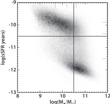
we split the foreground sample by mass at M 3 1010M
= ´
(about 1/2 L*; see Figure7). The average stellar mass of the low-mass group is6´109M 0.1
L*while the average for
the high-mass group is6´1010M
L*. We call these groups
the 0.1L*and L*sub-samples, respectively.
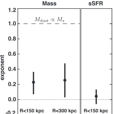
We determine the CGM reddening for each subsample and their ratios, shown in Figures 8 and 9, respectively. In determining the ratio we make the explicit assumption that the ratio of reddening to dust column is not a function of physical parameter by which we split the sample. We use all colors and covariances, as per Section 3.4. We detect more reddening around L* galaxies over our fiducial impact parameter range (30–150 kpc), but only by a factor of 1.7-+0.50.7.If we characterize this ratio as a power-law dependence
of CGM dust mass on host stellar mass wefind
MdustµMb withb=0.23-+0.150.15. ( )6
Figure 7. Bivariate distribution of foreground galaxies in sSFR and M . The
univariate quartile values are shown with long gray tickmarks; the splits used in Section4.2are shown in black.
Figure 8. Average reddening between 30 and 150 kpc impact parameter of foreground galaxies,DCdust(30 kpc, 150 kpc ,) split into sub-samples by stellar mass(top panel) and specifc star formation (bottom panel). In the top panel the blue half-circles and errors represent the measurement of a sub-sample with an average stellar mass of L*(the L*sample), while the red half-circles and errors represent the sub-sample with an average stellar mass of 0.1 L*(the 0.1 L* sample). In the bottom panel the blue half-circles represent the high specific star formation rate sub-sample, at an average of 2× 10⁻¹⁰yr−1, while the red half-circles and errors represent the low specific star formation rate sub-sample, at an average of 8× 10⁻¹²yr−1. It is visually evident that the higher mass galaxies produce more reddening, but not 10 times as much, as would be expected if CGM dust mass scaled linearly with galaxy stellar mass. No reddening trend is detectable as a function of sSFR.
The ratio does not change significantly when we increase the range of the impact parameter to 300 kpc, indicating that a more extended dust distribution around L* galaxies does not explain this weak dependence of CGM reddening with galaxy mass. We rule out a linear proportionality between Mdust and
M at a level greater than 4σ over this mass range.
We repeat the experiment, splitting the galaxy population by sSFR at 3× 10⁻¹¹yr−1(Figure7). The low sSFR subpopulation has an average sSFR of 8× 10⁻¹²yr−1 while the high sSFR subpopulation has an average sSFR of 2× 10⁻¹⁰yr−1. The trend with sSFR is characterized by Mdust sSFR with 0.04 0.09. 7 0.10 ( ) g µ g = -+
This is also reported in Figure9. It indicates that star forming and passively evolving galaxies surrounded by a similar distribution of dust in their halo.
5. DISCUSSION
Characterizing dust reddening effects at a level below one percent is challenging. A number of effects unrelated to dust can bias the measurements: physical clustering and gravita-tional lensing-induced color changes due to possible bright-ness-color trends (Section 3.1), large-scale photometric variations (Section 3.2), and offsets in the estimation of the sky background level near extended sources (Section 3.3). In this analysis we have accounted for these effects by using an estimator sensitive the excess reddening as a function of angular separation and only accounting for color changes affecting background sources (Equation (4)). Our results provide a new line of evidence that a substantial amount of dust resides in galactic halos (Section 4). As opposed to previous statistical studies using quasars as background sources (e.g., Chelouche et al. 2007; Ménard et al. 2010) we have
shown that it is possible to use background galaxies, and in particular standard crayons(Bovy et al.2008), PG10.
5.1. The Spatial Distribution of CGM Dust
The increased reddening detected within 150 kpc(Figure5) appears at first to be inconsistent with the smooth power-law found by MSFR. However, the MSFR result assumes that all of the foreground galaxies in that work are at z= 0.36 (Equation (22) of that work), while in fact it is based on photometrically detected foreground galaxies over a very broad range of true redshifts (Sheldon et al. 2012). Thus, any radial edge in the CGM in physical space around MSFR galaxies is washed out in angular space by the variation in redshift.
The increased detection within 150 kpc is qualitatively consistent with absorption lines of highly ionized metals (Wakker & Savage 2009) and cooler metals in the CGM (Bordoloi et al. 2011). These measurements of dust spatial distribution present an interesting and coherent picture to test against galaxy formation scenarios.
5.2. Trends with Galaxy Properties
A new frontier reached in this analysis is the ability to probe the relation between the amount of CGM dust and galaxy properties. Our results indicate no detectable relationship between sSFR and CGM dust content(Equation (7), Figure9). This result has implications for dust lifetime in the CGM and feedback mechanisms. Our blue sample has a sSFR 25 times higher than the red sample, and yet we detect no change in the amount of reddening signal.
If dust is primarily ejected from galaxies by star formation, and if star formation has not happened in quiescent galaxies for gigayears (Kauffmann et al. 2003), the ejected dust must survive in the CGM for a similar amount of time. This is consistent with the dust sputtering timescales predicted for
hot environments, 1010 a 0.1 m n 10 cm
H 5 3 1
( m )( )
~ - - - years
(Draine & Salpeter1979).
We also find that Mdust,CGMµMb with β ∼ 0.2
(Equa-tion(6), Figure9). This trend provides us with a new constraint for the modeling of galactic winds (Murray et al. 2005; Oppenheimer & Davé2006; Zu et al.2011) and metal pollution on large scales. We note that recent studies of CGM metals through absorption line analyses also point to a weak dependence on galactic stellar mass (Werk et al. 2013; Zhu & Ménard2013).
5.3. The Metal Budget
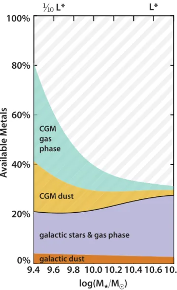
Determining the location and state of metals can help us understand how galaxies produce and expel material, and therefore how they evolve. While early work highlighted the location of metals at high redshift (e. g. Bouché et al. 2007), recently a complete analysis has been done by Peeples et al. (2014, P14). This work determined the total mass of metals formed by a galaxy by z∼ 0 as a function of Mthat were not
immediately locked in stellar remnants (Fukugita & Pee-bles2004): the “available metals.”P14showed that only∼25% of these available metals are detected within galaxy disks, and that some, but not all, are detected in the gas-phase of the CGM. This is the “missing metals” problem at low redshift: most metals created by stars over cosmic time are not detected. To illustrate the significance of CGM dust to the overall metal budget, we show a new version ofP14Figure9including
Figure 9. Dependence of circumgalactic reddening on galaxy properties. The left panel shows the exponentβ characterizing the dependence on stellar mass MdustµM ,b as a function of scale. The right panel shows the exponentγ
our measurement of the very weak dependence of CGM dust mass on host galaxy stellar mass (Figure 10), using the measurement from Ménard et al.(2010) that a galaxy of stellar mass1010.4M
has a CGM dust mass of5´107M(which is
consistent with our measurement). A number of assumptions go into this figure which are discussed at length in P14. Importantly, P14 assumes no dependence of CGM gas-phase metal mass on M(β = 0). However, observations of OVI and
lower ions can only rule out a linear, or stronger, dependence on M(rule outb 1). Part of this uncertainty stems from the
relatively few low-mass galaxies observed in the COS-Halos data set: only four in the range4 109M M 1010M
´
(Tumlinson et al. 2013). Our work presents a more precise measure of CGM dustβ (Equation (6)), in part due to the much larger range of foreground galaxy masses probed.
While each of these β measurements are subject to various independent uncertainties and biases, the fact that all three measurements (OVI ions, lower ions, and dust) show weak dependence on M in this mass range suggests that it is worth
examining the physical implications. With these fiducial
assumptions, a large fraction of the metals produced by 0.1 L* galaxies resides in the CGM, weakening any “missing metals” problem at that mass. Indeed, a 0.1 L*galaxy contains approximately as much metal in CGM dust as in the entire galaxy itself. Conversely, very little of the available metals from L* galaxies are found in detected phases of the CGM, suggesting that the missing metals must be in some unprobed phase or outside the CGM. These results give a valuable perspective on galaxy formation models, especially in the context of galactic feedback.
6. CONCLUSION
We can draw several conclusions from this work.
1. Using galaxies and in particular standard crayons as background sources we detect the excess reddening induced by the extended distribution of dust around galaxies.
2. We confirm the existence of~ ´6 107M
of dust in the
CGM of 0.1 L*–L*galaxies, consistent with the results of MSFR based on reddening of background quasars. 3. We find a weak dependence of CGM dust reddening on
galaxy stellar mass MdustµM0.2(Equation (6)), and no
detectable dependence on sSFR.
4. Including constraints on the distribution of metals from absorption line studies, the dust contribution to the overall metal budget indicates that the missing metals problem at low redshift is more acute near L* galaxies than near 0.1 L*galaxies.
We have found in this work that the photometry of close pairs of galaxies is susceptible to significant systematic error, even in a survey with photometry tested as meticulously as the SDSS (Padmanabhan et al. 2008). These systematics, and other possible unknown systematics, should be considered seriously, and we hope to confirm the above conclusions with future work. To press forward with the measurement of extragalactic dust reddening, we must build photometric pipelines that are resistant to the kinds of biases discussed in this paper. Future ground-based surveys and space missions may sidestep some issues with more stable seeing, darker skies, and higher resolution. However, without a clear specification to deliver photometry unbiased by close neighbors, we cannot assume that such surveys will be optimal for this measurement. Better bias constraints on the photometry of close pairs are also very important for weak lensing magnification measurements (Huff & Graves2013). An alternative is to use observations of color-standardized point sources (quasars) to study extragalactic reddening.
With these important caveats in mind, we look toward the future of measuring dust in the CGM of galaxies with spectroscopic galaxy data. Expanding the analysis to a broader range of wavelengths would help better constrain the dust extinction properties, perhaps including WISE (Wright et al. 2010) and GALEX (Martin et al. 2005) data. A preliminary investigation has shown much stronger systematic biases in close galaxy pairs when comparing photometry across surveys. Data from the GAMA survey(Driver et al.2011) may help us reach higher precision, especially because the multi-pass spectroscopic survey avoids fiber collision issues, and many more close pairs can be studied. BOSS (Dawson et al.2012) has observed 10 times more passively evolving galaxies than the original SDSS data, but its targets are selected with cuts in
Figure 10. Account of all available metals as a function of galaxy mass, from the analysis ofP14. Below the black line are metals in stars and the gas-phase ISM(purple), and ISM dust (orange). Above the black line are CGM metals: low-ions and OVI-traced metals (green) and CGM dust from this work (yellow). The hashed area represents metals missing from galaxies themselves. There is a very clear difference in the fraction of metals accounted for in 0.1 L* galaxies vs. L* galaxies. For a discussion of uncertainties on these values seeP14.
color space, which may contaminate the standard crayons. If this contamination can be well understood, BOSS may allow us to study CGM reddening at z ∼ 0.5. Future surveys like the notional high latitude survey proposed for WFIRST (Spergel et al.2013) may allow similar measurements toward z ∼ 2, at the height of galaxy formation in the history of the universe.
We thank Daniel Rabinowitz of the Columbia statistics department for sage wisdom and Eric Huff and Genevieve Graves for insight into issues in the SDSS photo pipeline. We thank Jessica Werk for insight into COS-Halos mass dependence and Molly Peeples for providing the data from Peeples et al.(2014) for Figure 10.
J.E.G.P. was supported by HST-HF-51295.01A, provided by NASA through a Hubble Fellowship grant from STScI, which is operated by AURA under NASA contract NAS5-26555. B.M. is supported by NSF Grant AST-1109665 and work by L.R.C. was supported by NASA Headquarters under the NASA Earth and Space Science Fellowship Program, grant NNX11AO09H.
Funding for the Sloan Digital Sky Survey (SDSS) and SDSS-II has been provided by the Alfred P. Sloan Foundation, the Participating Institutions, the National Science Foundation, the U.S. Department of Energy, the National Aeronautics and Space Administration, the Japanese Monbukagakusho, and the Max Planck Society, and the Higher Education Funding Council for England. The SDSS Web site is http://www. sdss.org/.
The SDSS is managed by the Astrophysical Research Consortium (ARC) for the Participating Institutions. The Participating Institutions are the American Museum of Natural History, Astrophysical Institute Potsdam, University of Basel, University of Cambridge, Case Western Reserve University, The University of Chicago, Drexel University, Fermilab, the Institute for Advanced Study, the Japan Participation Group, The Johns Hopkins University, the Joint Institute for Nuclear Astrophysics, the Kavli Institute for Particle Astrophysics and Cosmology, the Korean Scientist Group, the Chinese Academy of Sciences(LAMOST), Los Alamos National Laboratory, the Max-Planck-Institute for Astronomy(MPIA), the Max-Planck-Institute for Astrophysics (MPA), New Mexico State Uni-versity, Ohio State UniUni-versity, University of Pittsburgh, University of Portsmouth, Princeton University, the United States Naval Observatory, and the University of Washington.
REFERENCES
Aihara, H., Allende Prieto, C., An, D., et al. 2011,ApJS,193, 29
Blanton, M. R., Eisenstein, D., Hogg, D. W., Schlegel, D. J., & Brinkmann, J. 2005,ApJ,629, 143
Bohren, C. F., & Huffman, D. R. 1983, Absorption and Scattering of Light by Small Particles(New York: Wiley)
Bordoloi, R., Lilly, S. J., Knobel, C., et al. 2011,ApJ,743, 10
Bouché, N., Lehnert, M. D., Aguirre, A., Péroux, C., & Bergeron, J. 2007,
MNRAS,378, 525
Bovy, J., Hogg, D. W., & Moustakas, J. 2008,ApJ,688, 198
Brinchmann, J., Charlot, S., White, S. D. M., et al. 2004,MNRAS,351, 1151 Burstein, D., & Heiles, C. 1982,ApJS,87, 1165
Chelouche, D., Koester, B. P., & Bowen, D. V. 2007,ApJL,671, L97 Cordiner, M. A., Cox, N. L. J., Evans, C. J., et al. 2011,ApJ,726, 39 Dawson, K. S., Schlegel, D. J., Ahn, C. P., et al. 2012,AJ,145, 10 Draine, B. T. 2003,ApJ,598, 1026
Draine, B. T., & Lee, H. M. 1984,ApJ,285, 89 Draine, B. T., & Salpeter, E. E. 1979,ApJ,231, 77
Driver, S. P., Hill, D. T., Kelvin, L. S., et al. 2011,MNRAS,413, 971 Efstathiou, G. 2000,MNRAS,317, 697
Fieller, E. C. 1954, J. R. Stat. Soc. Series B., 16, 2 Fukugita, M. 2011, arXiv:1103.4191
Fukugita, M., & Peebles, P. J. E. 2004,ApJ,616, 643 Hodges-Kluck, E., & Bregman, J. 2014,ApJ,789, 131
Holwerda, B. W., Keel, W. C., Williams, B., Dalcanton, J. J., & de Jong, R. S. 2009,AJ,137, 3000
Huff, E. M., & Graves, G. J. 2013,ApJL,780, L16
Kalberla, P. M. W., Burton, W. B., Hartmann, D., et al. 2005,A&A,440, 775 Kashiwagi, T., Yahata, K., & Suto, Y. 2013,PASJ,65, 43
Kauffmann, G., Heckman, T. M., Simon White, D. M., et al. 2003,MNRAS, 341, 33
Lan, T.-W., Ménard, B., & Zhu, G. 2014, arXiv:1404.5301 Laor, A., & Draine, B. T. 1993,ApJ,402, 441
Martin, D. C., Fanson, J., Schiminovich, D., et al. 2005,ApJL,619, L1 Ménard, B., & Fukugita, M. 2012,ApJ,754, 116
Ménard, B., Scranton, R., Fukugita, M., & Richards, G. 2010, MNRAS, 405, 1025
Murray, N., Quataert, E., & Thompson, T. A. 2005,ApJ,618, 569 Narayan, R. 1989,ApJL,339, L53
Oppenheimer, B. D., & Davé, R. 2006,MNRAS,373, 1265
Padmanabhan, N., Schlegel, D. J., Finkbeiner, D. P., et al. 2008, ApJ, 674, 1217
Peek, J. E. G. 2013,ApJL,766, L6
Peek, J. E. G., & Graves, G. J. 2010,ApJ,719, 415 Peek, J. E. G., & Schiminovich, D. 2013,ApJ,771, 68
Peeples, M. S., Werk, J. K., Tumlinson, J., et al. 2014,ApJ,786, 54 Roussel, H., Wilson, C. D., Vigroux, L., et al. 2010,A&A,518, L66 Salem, M., Bryan, G. L., & Hummels, C. 2014,ApJ,797, 18 Schlegel, D. J., Finkbeiner, D. P., & Davis, M. 1998,ApJ,500, 525 Scranton, R., Ménard, B., Richards, G. T., et al. 2005,ApJ,633, 589 Sheldon, Erin S., Cunha, E. Carlos, Mandelbaum, Rachel, et al. 2012,ApJS,
201, 2
Silk, J. 1997,ApJ,481, 703
Spergel, D., Gehrels, N., Breckinridge, J., et al. 2013, arXiv:1305.5425 Stoughton, C., Lupton, R. H., Bernardi, M., et al. 2002,AJ,123, 485 Strauss, M. A., Weinberg, D. H., Lupton, R. H., et al. 2002,AJ,124, 1810 Tumlinson, J., Thom, C., Werk, J. K., et al. 2013,ApJ,777, 59
Wakker, B. P., & Savage, B. D. 2009,ApJS,182, 378 Weingartner, J. C., & Draine, B. T. 2001,ApJ,548, 296
Werk, J. K., Prochaska, J. X., Thom, C., et al. 2013,ApJS,204, 17 Wright, E. L., Eisenhardt, P. R. M., Mainzer, A. K., et al. 2010,AJ,140, 1868 Yahata, K., Yonehara, A., Suto, Y., et al. 2007,PASJ,59, 205
York, D. G., Adelman, J., Anderson, J., et al. 2000,AJ,120, 1579 Zhu, G., & Ménard, B. 2013,ApJ,773, 16