A non-linear neural network technique for updating of river flow forecasts

HAL Id: hal-00304634

https://hal.archives-ouvertes.fr/hal-00304634

HAL is a multi-disciplinary open access archive for the deposit and dissemination of sci-entific research documents, whether they are pub-lished or not. The documents may come from teaching and research institutions in France or abroad, or from public or private research centers.

L’archive ouverte pluridisciplinaire HAL, est destinée au dépôt et à la diffusion de documents scientifiques de niveau recherche, publiés ou non, émanant des établissements d’enseignement et de recherche français ou étrangers, des laboratoires publics ou privés.

river flow forecasts

A. Y. Shamseldin, K. M. O’Connor

To cite this version:

A. Y. Shamseldin, K. M. O’Connor. A non-linear neural network technique for updating of river flow forecasts. Hydrology and Earth System Sciences Discussions, European Geosciences Union, 2001, 5 (4), pp.577-598. �hal-00304634�

A non-linear neural network technique for updating of river flow

forecasts

Asaad Y. Shamseldin

_{and Kieran M. O’Connor}

1Civil Engineering, The University of Birmingham, Edgbaston, Birmingham B15 2TT, United Kingdom 2Department of Engineering Hydrology, National University of Ireland, Galway, Galway, Ireland Email for corresponding author: [email protected]

Abstract

A non-linear Auto-Regressive Exogenous-input model (NARXM) river flow forecasting output-updating procedure is presented. This updating procedure is based on the structure of a multi-layer neural network. The NARXM-neural network updating procedure is tested using the daily discharge forecasts of the soil moisture accounting and routing (SMAR) conceptual model operating on five catchments having different climatic conditions. The performance of the NARXM-neural network updating procedure is compared with that of the linear Auto-Regressive Exogenous-input (ARXM) model updating procedure, the latter being a generalisation of the widely used Auto-Regressive (AR) model forecast error updating procedure. The results of the comparison indicate that the NARXM procedure performs better than the ARXM procedure.

Keywords: Auto-Regressive Exogenous-input model, neural network, output-updating procedure, soil moisture accounting and routing (SMAR) model

Introduction

The present paper deals with the application of the neural network technique as an updating procedure for river flow forecasts and with the assessment of its performance by comparison with some of the well established updating procedures.

In the context of river flow forecasting, the estimated discharge hydrographs of the rainfall-runoff simulation models normally differ, often substantially, from the corresponding observed discharge hydrographs. These differences (i.e. the discharge forecast errors) are attributable to many factors which include: (1) inadequacy of the structure of the rainfall-runoff simulation model to represent the constituent hydrological processes (i.e. model inadequacy or error), (2) poor estimation of the model parameters (due to inefficiency or failure of the optimisation procedures) and (3) both systematic and random errors in the model input and output data (Becker and Serban, 1990, p. 29). Perhaps less generally acknowledged or emphasised by hydrological modellers is the fact that the poor performance of a model may also reflect inadequacy in the

information carrying capacity of the data available to calibrate and operate the model, i.e. the quality of the data applied to the model (in the sense of being truly representative, as distinct from measurement errors in such data) may be simply insufficient to support the level of structural complexity of the model to which these data are applied (Klemes, 1988). This could arise, for example, in the context of a conceptual model, either from inadequate spatial or temporal resolution of the available data such as the lumping of rainfall as a single time series or, in the case of a semi-distributed model, from the inappropriate adoption of a representative elementary area (REA) over which the hydrological variables are assumed to be uniform (Wood et

al., 1988). Ironically, the more serious and scientific the

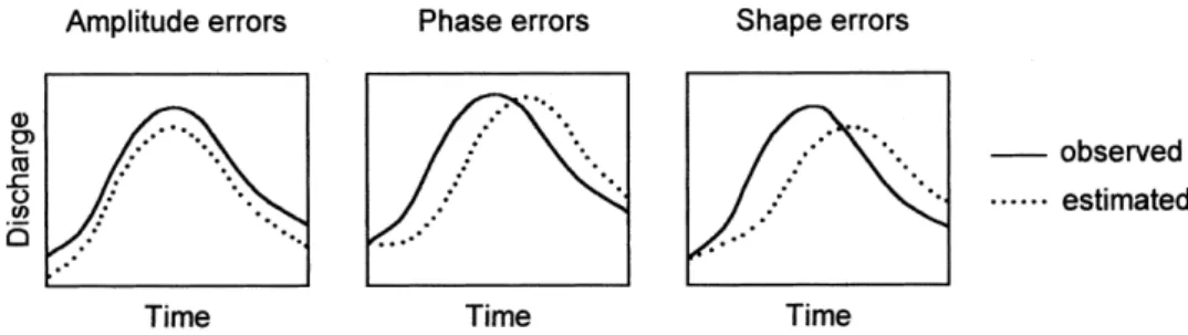
attempt of the modeller to represent faithfully the physical processes involved in the transformation of rainfall to runoff, i.e. the greater the hydrological substance of the model, the more likely will the performance potential of the model be adversely affected by the data-inadequacy phenomenon. The errors between the simulated and the observed discharge hydrographs can be categorised into three types (Serban and

Askew, 1991), namely, volume (amplitude) errors, phase errors and shape errors (see Fig. 1). The volumetric errors reflect the over-estimation or under-estimation of the flood hydrograph volume and may be due to errors in the input data and structural deficiencies in the water-balance module of the substantive rainfall-runoff model. The phase errors express the inaccuracies in the timing of the flood hydrograph whereby the near-correct numerical values of the discharge are estimated but are either delayed or advanced in time. Although the phase error is of only marginal significance in most simulation mode applications, it is crucial in the real-time forecasting scenario in which it can be the deciding factor in adopting or rejecting a model. Both the shape and the phase errors are mainly induced by the inability of the routing module of the model to provide a satisfactory redistribution of the generated runoff volumes over time. In practice, various combinations of these three types of error may occur.

Non-linear lumped forecasting models of the conceptual and black-box types are traditionally calibrated off-line, using historical data. In operation, they may be run either in simulation/design mode (without updating, i.e. without incorporating any feedback in the form of the observed discharges immediately prior to the time of issuing the forecast) or in real-time updating mode (as the substantive simulation model coupled with its corresponding error-forecasting procedure). In the former case, only the physical inputs to the process being modelled are used (e.g. rainfall with or without evaporation) and no real-time updating of the forecast is involved. Such, for example, would be the case in simulating the model output (i.e. the discharge) either for the calibration period or for the verification/validation period, this operation being performed off-line. In contrast, in the real-time river flow forecasting scenario, the same calibrated rainfall-runoff simulation model operates on-line, utilising the current and most recently available physical-input data, a separate add-on forecast-updating procedure being used to partially compensate for the inevitable errors between the discharge forecasts of that simulation model

and the corresponding observed discharge values. Such a forecast-updating procedure is designed and applied specifically to facilitate the use of feedback information (in the form of the most recently observed discharge data) in order to refine or enhance the discharge forecasts of the substantive model. It is usually calibrated off-line using the output series of the substantive model, over its calibration period, and the corresponding observed discharge values. The substantive simulation model, operating together (i.e. coupled) with its output forecast updating procedure, is known as a real-time forecasting model (Becker and Serban, 1990, p. 29). The ability of real-time forecasting models to respond and adapt to such feedback information is a unique characteristic of such models. The two parts of the real-time forecasting model (i.e. the substantive simulation model and the updating procedure) are complementary and any real-time hydrological forecasting model is incomplete without an updating procedure. The estimated discharges produced by the substantive simulation model, without any

updating, are generally referred to as the simulation (design) mode discharge forecasts, while those obtained

subsequently after applying the updating procedures are referred to as the updating mode discharge forecasts.

Traditionally, the prospect of the enhancement of the simulation mode discharge forecasts that may be achieved by improving the structure of the substantive rainfall-runoff simulation model has received considerably more attention than that of the subsequent enhancement of such forecasts to be obtained by improving the structure of the corresponding forecast-updating procedure. This imbalance in research activity probably reflects the perception that there is more scope and scientific challenge in refining the substantive rainfall-runoff model than the less scientifically respectable black-box constructs of the updating procedure. This perception is also reflected in the large number of recent publications dealing with developments and modifications of rainfall-runoff models (e.g. Seibert et al., 2000; Hromadka II, 2000; Jayawardena and Zhou, 2000; Yue and Hashino, 2000; Houghton-Carr, 1999; Thyer et al., 1999; Kuczera Fig. 1. Types of error between estimated and observed discharge hydrographs

and Parent, 1998; Mroczkowski et al., 1997; Ye et al., 1997; Franchini and Galeati, 1997; Yapo et al., 1996; Gan et al., 1997; Lauzon et al., 1997; Lamb, 1997; Sumner et al., 1997; Cooper et al., 1997; Todini, 1996). Although considered of secondary importance, notable attention has also been focussed on procedures for updating the substantive model forecasts, particularly by international hydrological organisations such as the World Meteorological Organisation (WMO) (WMO, 1992). While an improvement of the structure of the substantive model would generally be anticipated to result in increased forecasting accuracy for both longer and shorter forecast lead-times, an improvement in the updating procedure can generally be expected to enhance substantially the forecasting accuracy of the model for short-term forecasting only. This is nevertheless a worthy objective as accurate and reliable short-term forecasting is essential for the day-to-day management and operation of real-time river flow forecasting systems and such systems provide information which is essential for minimising the hazardous impacts of floods, etc. It is in this context that the present work on the use of the neural network technique as a river flow forecasting updating procedure has been undertaken.

While the real-time river flow updating procedures in operational use differ in details, these updating procedures may, however, be classified depending on the type of model variables to be modified. The variables are: (1) the model input variables, (2) the model output variables, (3) the model parameters and (4) the constraints and thresholds operating on the water contents of the various storage elements of the model (Moore, 1986). Some of the real-time river flow forecasting models may modify more than one such type of model variable (Becker and Serban, 1990, p. 31; Serban and Askew, 1991; WMO, 1992, p. 11). The proper choice of an updating procedure depends on the user requirements, the amount and the quality of the data available, the equipment used for the data collection, transmission and processing and also on the experience and the expertise of the personnel responsible for making the forecasts (WMO, 1994, p. 585). However, there is still no universal consensus on the best type of updating procedure for river flow forecasting (cf. WMO, 1992; Refsgaard, 1997).

The present study deals only with model-output updating procedures. These updating procedures modify externally the simulation mode discharges in real-time without interfering with the operation of the substantive rainfall-runoff simulation model. In using such procedures, there is no need, therefore, for re-running the substantive model or for modifying the parameters and the water contents of the internal storage elements of that model. Such output updating procedures are generally considered to be simpler

and easier to use than the other types of updating procedures. One of the simplest and most widely used model-output updating procedures is that which involves the forecasting of the errors in the simulated discharge values of the substantive rainfall-runoff model (cf. Serban and Askew, 1991; Ahsan and O’Connor, 1994) using a simple linear

Auto-Regressive (AR) time series model. In this procedure,

an AR model is separately calibrated off-line to the error time series of the simulation mode discharge forecasts (i.e. to the series of differences between the un-updated simulation mode forecasts and the corresponding values of the observed discharge series) and subsequently it is used in real-time for forecasting the errors in the simulation mode discharge forecasts. These error forecasts are then simply added to the non-updated (simulation-mode) discharge values to give the required updated discharge forecasts. Thus, the AR updating may be regarded as an indirect method of updating, as the updated discharge forecast values so obtained are computed in an indirect manner. The success of the AR updating procedure is dependent mainly on the

degree of serial correlation in the forecast error time series

of the substantive runoff model (Serban and Askew, 1991; Shamseldin, 1996; Moore, 1999).

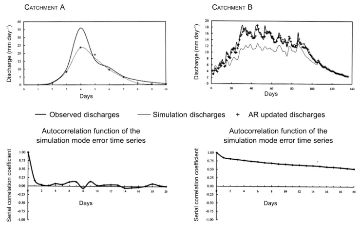
Figure 2 shows examples of AR error updating for two catchments, denoted simply by the letters A and B. In catchment A, the simulation-mode error time series does not display high persistence, since the serial autocorrelation coefficient values for non-zero lags are not significantly different from zero. However, in the case of catchment B, the corresponding error series has high persistence, the corresponding serial correlation coefficient values being significantly different from zero. Examination of Fig. 2 shows that the AR updating is indeed successful in the case of catchment B, since the updated discharges match the observed discharges much more closely than those of the simulation mode. However, in the case of catchment A, the simulated and the updated discharges are not that different and therefore the AR-updating does not improve substantially the quality of the discharge forecasts for this catchment. These examples illustrate that AR updating is only successful when the structure of the simulation-mode error time series exhibits high serial correlation.

Shamseldin and O’Connor (1999) noted that the mathematical formulation of the AR forecast error-updating procedure is a special limiting case of the more general input-output procedure, which is based on the structure of the linear Auto-Regressive Exogenous-input (ARXM) model, also known as the Linear Transfer Function Model (LTFM). In the ARXM updating procedure, the simulation mode (i.e. non-updated) discharge time series produced by the substantive rainfall-runoff model constitutes the exogenous

Fig. 2. Examples of AR error updating

CATCHMENTA CATCHMENT B

Observed discharges Simulation discharges + AR updated discharges

Autocorrelation function of the simulation mode error time series

Autocorrelation function of the simulation mode error time series

Discharge (mm day

–1)

Discharge (mm day

–1)

Serial correlation coef

ficient

Serial correlation coef

ficient

Days Days

Days Days

input, which is used together with the available observed discharges in providing the updated discharge forecast. Thus, the main difference in the operation of the ARXM and the AR error-updating procedures is that the former directly produces the updated discharge forecasts as outputs whereas the latter provides estimates of the simulation discharge forecast errors.

Since the ARXM updating procedure is more general than the AR model updating procedure, the ARXM updating procedure is used in the present study as a convenient benchmark against which the performance of the non-linear neural network updating procedure can be compared. The daily estimated discharge forecasts of the lumped conceptual Soil Moisture Accounting and Routing (SMAR) model (O’Connell et al., 1970; Kachroo, 1992; Khan, 1986; Liang, 1992) for five catchments of different sizes and climatic conditions are used in this comparison of updating procedures. Three of these five catchments are located in China, the remaining two catchments being located in Ireland and Thailand.

In the present paper, the neural network technique is investigated as an alternative model-output updating procedure to that of the ARXM. This is done to test whether or not the greater complexity afforded by the neural network

updating procedure is warranted for updating the discharge forecasts of the substantive rainfall-runoff model. Neural networks may be regarded as a mathematical technique which was inspired by research on biological networks. In general, the network is composed of a number of linear and non-linear computational units (neurons), which operate as one group in the process of input-output transformation. Thus, neural networks may be viewed purely as non-linear black-box models and similar to the application of such models they are calibrated using a synchronous set of actual observed input and output data. The technique is non-parametric (i.e. data-driven) (Maier and Dandy, 1996; Fortin

et al., 1997) in the sense that there is no a priori assumption

made about the specific mathematical form of the function relating the inputs and the outputs (Azof, 1994, p. 1). It is recognised as being very powerful for modelling complex non-linear problems (Maier and Dandy, 2000; Brion and Lingireddy, 1999; Azof, 1994, p. 3) and for being relatively insensitive in operation to errors in the data (Hammerstrom, 1993). These attractive characteristics have motivated the present authors to investigate the neural network technique as a runoff model output updating procedure.

There are various forms of neural networks available (Lippmann, 1987; Maren, 1990, pp. 53-57; Skapura, 1995,

pp. 29-64). However, for the present study, a multi-layer feedforward neural network (MLFNN) is selected as an output updating procedure and it has been chosen mainly for its flexibility in function approximation (Hecht-Nielsen, 1991, p. 131). The MLFNN uses the same input information and produces similar output information to that of the ARXM model-output updating procedure already described. In this context, the MLFNN updating procedure may be viewed as being analogous in its mathematical structure to a non-linear form of Auto-Regressive Exogenous-input model (NARXM) (Bomberger and Seborg, 1998; Previdi

et al., 1999; Yu et al., 2000). In so doing, the term

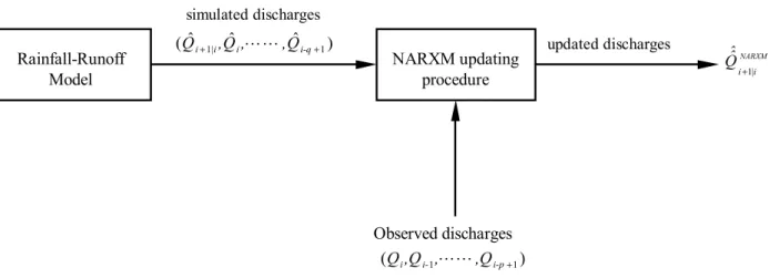
‘auto-regressive’ is being used in its broadest sense of describing an output forecast updating technique utilizing the recently measured outputs and as such is not to be confused with the standard statistical techniques of linear and non-linear regression analysis. Reflecting this structural analogy, it is henceforth referred to in this study as the NARXM updating procedure. Thus, the NARXM updating provides a methodology for integrating neural networks and substantive rainfall-runoff models. Similar to the ARXM updating procedure, the NARXM updating procedure is also direct in the sense that it produces the updated discharge forecasts as its output. A schematic diagram of the operation of the NARXM updating procedure is provided in Fig. 3.

The present paper is organised in the following manner; firstly, a description of the ARXM and the NARXM updating procedures is given. Secondly, the structure of the SMAR conceptual model is outlined, this model having been selected for convenience as the substantive rainfall-runoff simulation model. Finally, a description is provided of the application of the ARXM and the NARXM updating procedures to the estimated daily discharge series of the SMAR model, for the five selected catchments, and the

performances of these two updating procedures are compared.

The Auto-Regressive

Exogenous-input Model (ARXM) updating

procedure

The Auto-Regressive Exogenous-input Model (ARXM) is a linear input-output model which enables the forecasting of the future values of a time series on the basis of its recent past values and on the basis of the values of one or more exogenous input times series. Due to its flexibility, in addition to being parsimonious in the number of parameters employed, the ARXM has been applied widely as a river flow-forecasting model (e.g. O’Connell and Clarke, 1981; Galeati, 1990; Hsu et al., 1995; Moore, 1999). In such applications, the exogenous inputs to the model are the traditional physical input sources such as rainfall and, if appropriate, the upstream inflow hydrograph. However, in the application of the ARXM as a rainfall-runoff model output updating procedure, the exogenous inputs to the ARXM are the simulation mode discharge forecasts, Qˆi, of

the substantive rainfall-runoff model (i.e. the SMAR model in the present study).

The ARXM model-output updating procedure was originally suggested by Peetanonchai (1995) and subsequently investigated by Abdelrahman (1995), Shamseldin (1996), Suebjakla (1996) and Shamseldin and O’Connor (1999). The one-step-ahead (i.e. that for a forecast lead-time of one data interval) ARXM output updating procedure, incorporating a residual updated discharge forecast error term ARXM

1 i

e

+ , can be expressed mathematically

as;

Fig. 3. Schematic diagram of the operation of the NARXM prodcedure for forecast origin i for one-step ahead NARXM updating procedure Rainfall-Runoff Model simulated discharges updated discharges Observed discharges ) (Qi,Qi-1,LL,Qi-p+1 ) ˆ ˆ ˆ (Q_i+1|i,Q_i,_LL,Q_i-q+1 NARXM i i Qˆˆ | 1 +

ARXM i k i q k k k i p k k i aQ bQˆ e Q 1 1 0 1 1 1 −+ ₊ = + − = + =

∑

∑

In this equation, Qi+1 denotes the as-yet-unmeasured

discharge for the (i+1)st _{time step, the updated}

one-step-ahead discharge forecast ( ARXM |i i

Q

1 ˆˆ

+ ) made at the current i th _time

step having the form

ˆ ˆ ˆˆ 1 1 1 0 1 1 1 1 1 Q e a Q bQ bQ Q q k k i k |i i k i p k k i i |i i ARXM ARXM

∑

∑

where the Q_i-k+1 are the current and most recently observed discharges, Qˆi+1|i is the one-step-ahead simulation mode

discharge forecast of the substantive rainfall-runoff model, the Qˆi−k+1 values are the current and recent outputs of that

model, p and q are the orders of the auto-regressive and the exogenous input parts of the ARXM, respectively, a_kand b_k being the corresponding coefficient parameters of these two parts. Note that, operating in real time, some forecast of the rainfall (meteorological or otherwise, with or without the corresponding forecast of evaporation) is required to obtain the un-updated one-step-ahead forecast value Qˆi+1|i.

Equation (2) may be regarded simply as a multiple-linear-regression type of model. Thus, the parameters of the ARXM can be estimated directly using the method of ordinary least squares.

In operational river flow forecasting systems, a generalization of Eqn.(2) can be used on-line to provide the updated discharge estimate ARXM

l|i i

Qˆˆ

+ for the required forecast

lead-time l >1 (i.e. for the period beyond the current time i at which the forecast is required). Hence updated estimates of the values of the discharges over the lead-time of the forecast are required as well as the non-updated outputs of the substantive rainfall-runoff model over that lead-time, including that at the (i+l)th _{time step. In real-time}

applications, these non-updated outputs over the lead-time are obtained using forecasts of the meteorological (e.g. rainfall, evaporation, etc.) input estimates. As the values of the observed discharges over the forecast lead-time are by definition not yet available, the updated estimates of these values are used instead, where these are generated by recursive application of Eqn.(2). Thus, at time-step i, the updated discharge forecast, ARXM

i| l i Qˆˆ + , for a lead-time l>1, is given by ˆ ˆ ˆˆ ˆˆ 1 0 1 1 Q b Q b Q a Q a Q q l k k l i k l k k|i l i k k l i p l k k l k il k|i k l|i i ARXM ARXM

∑

∑

∑

∑

As the focus of the present study is on the introduction of the NARXM forecast updating procedure and on the comparison of its results with those of the ARXM procedure, the scenario of ‘perfect foresight of input over the lead-time

of the output forecast’ was adopted in the computation of

the corresponding non-updated discharge forecasts of the substantive rainfall-runoff model, i.e. instead of using the forecasts of the meteorological (e.g. rainfall, evaporation, etc.) input to that model, the actual meteorological input data over the lead-time are used, this input scenario having also been used for its calibration. This choice of input scenario effectively eliminates the effects on the updating models of errors in the meteorological forecasts when these are used as inputs to the substantive model, so that the relative merits of the selected forecast-updating procedures can be assessed more objectively. In real-time applications, however, the imperfect meteorological forecasts must be used and undoubtedly the introduction of this additional source of input error over the forecast lead-time will adversely affect the overall efficiency of the real-time forecasting system. Quite deliberately, in this paper, the complicating effects of this or indeed other possible choices of input-over-lead-time scenarios, such as the assumption that the current input remains constant over the forecast lead-time, are not introduced, only the ‘perfect foresight of input

over the lead-time of the output forecast’ scenario being

considered.

The Non-linear Auto-Regressive

Exogenous-input Model

(NARXM)-neural network updating procedure

The neural network technique is applied in the present study as an alternative procedure to that of the ARXM for updating the discharge forecasts of the substantive rainfall-runoff model. In non-parametric form, the one-step-ahead NARXM-neural network updating procedure may be expressed as NARXM i i-q i i i i-p i-i i hQ,Q , ,Q ,Q ,Q, ,Q e Q+1= ( 1LL +1 ˆ+1| ˆ LL ˆ +1)+ ₊₁ (4)

in which h denotes a non-linear functional relation and

NARXM

i

e

1

+ is the residual error of the corresponding updated discharge-forecast NARXM i i Qˆˆ | 1 + , where NARXM NARXM i i i i Q e Qˆˆ_+1| = +1− +1 .

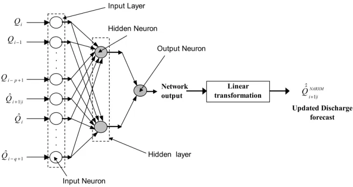
Figure 4 shows the general structure of the multi-layer feedforward neural network used in the present study. The multi-layer feedforward network consists of a number of layers of neurons (computational units), which are linked by connection pathways. Each layer of neurons has a unique role in the overall operation of the network. The neurons within the same layer have no inter-connection pathways. All the neurons within each layer function in a similar fashion and have a similar pattern of connection pathways to the neurons in the adjacent layer/layers. Each neuron can

have a multiple-input but it produces a single output. The connection pathways provide the means for transferring the information between the different neurons in the adjacent layers. The network may be viewed as a collection of sub-models (neurons), which work collectively to transform the external inputs to the network into its output.

The layers making up the network are the input layer, the output (external) layer and the hidden layer, which is intermediate between the input and the output layers. In general, the multi-layer feedforward network can have more than one hidden layer. However, the use of a single hidden layer is generally recommended (Masters, 1993, pp. 174-180) and this recommendation has been adopted in many of the applications of the multi-layer feedforward networks to the field of hydrology and water resources (Luk et al., 2000; Lange, 1999; Thirumalaiah and Deo, 1998; Shamseldin et al., 1997; Maier and Dandy, 1996; Minns and Hall, 1996; Hsu et al., 1995). Accordingly, one hidden layer is used in the present study.

The input layer receives the external input array to the network and each of the elements of this array is designated to one (and only one) of the input neurons. In the case of one-step-ahead forecasting, the external inputs (i.e. the exogenous inputs) to the network are the simulation-mode discharge forecasts Qˆ_i+1|i,Qˆ_i,_LL,Qˆ_i-q+1 and the current and previous recently observed discharges Qi,Qi-1,LL,Qi-p+1.

Each neuron in the input layer produces a single output that, in its entirety, becomes an input to each of the neurons in

the subsequent (hidden) layer. The input-output transformation for each input neuron is achieved by a direct transformation in which the output of each neuron is equal to its external input. Therefore, the main role in the overall operation of the network is simply to provide a mechanism to transmit the external input array into the network.

The hidden layer is the intermediate layer between the input and the output layers. In general terms, the hidden layer usually enhances the ability of the network to model non-linear processes (Medsker, 1994, p. 12). The hidden neurons, in the case of the multi-layer feed-forward network, have no direct connection pathways to either the external inputs or outputs of the network. The number of neurons in the hidden layer is initially unknown. The optimum number is usually estimated by a trial and error procedure in which the network is calibrated (i.e. trained) successively with an increasing number of hidden neurons, the performance of the network being monitored in each trial using the chosen index of performance. The selected optimum number of neurons in the hidden layer is generally that beyond which the performance of the network does not substantially improve with an increase in that number. Each hidden neuron has an input array, which consists of the outputs of the input layer neurons. The hidden neuron produces only a single output, which becomes an element of the input array to each neuron in the following layer. The transformation of its input array, by each neuron of the hidden layer, to a single output is achieved by a mathematical non-linear transformation Fig. 4. Schematic diagram for the multi-layer feedforward Neural Network used as an output updating procedure for one-step-ahead

Network output Hidden layer Input Layer Output Neuron Hidden Neuron Input Neuron Linear transformation Updated Discharge forecast . . . . . . 1 − i

Q

Q

Qˆ

Q

ˆˆ

function, which introduces non-linearity into the operation of the network. The same transformation function is normally used for all of the hidden layer neurons. The mechanism of the transformation for each of these hidden layer neurons can be expressed mathematically as (Shamseldin et al., 1997) ) w y w f y M _{i o} i i out

∑

in which yout is the hidden neuron output, f() is the

non-linear transformation function, M is the total number of the number of neurons in the previous (input) layer, w_i is the connection weight which is assigned to the connection pathway between the hidden layer neuron and the i-th neuron in the previous (input) layer, y_i is the input to the neuron (and to the corresponding neuron of the previous input layer), and w₀ is the threshold (constant bias or intercept) of the neuron. In general, each neuron has its own set of weights and threshold value. The weights and the threshold values of the various neurons are, in effect, the parameters of the network. The total number of such parameters is governed directly by the number of neurons forming the network.

A number of non-linear transformation functions has been suggested for use in conjunction with neural networks (Fausett, 1994, pp. 17-19; Masters, 1993, pp. 81-82). The most widely used transformation function is the logistic function. Accordingly, the sigmoid function is adopted in the present work. The logistic function has an S shape and its values vary between 0 and 1. This function may conventionally be expressed as o i M i wiy w o i M i i out f wy w y + ∑ + =

∑

The output layer is the last layer in the network and its main role is to produce the final output array of the network. In the present study, the output layer has a single neuron as only one output is required. The process of the transformation of the input array to a single output, for that output layer neuron, is similar to that of the hidden neuron, which is expressed by Eqn. (5). Thus, the transformation is achieved using the logistic function defined by Eqn.(6). Since the logistic function is bounded in the interval [0,1], this would imply that the final network output is also bounded in this interval. In practice, however, in order to alleviate some of the numerical difficulties that may arise, especially when derivative-based optimisation methods are used for training (i.e. calibrating) the network, the effective range is generally less than the above interval. In the present study, the following linear function, which was also adopted by Shamseldin et al. (1997), is used for rescaling the actual observed discharges, giving

) ( 75 0 1 0 max Q Q . + . = Qs i i (7)

where Qs_i is the re-scaled series, Qiis the corresponding

observed discharge and Qmax is the maximum observed

discharge in the calibration period. In accordance with this linear rescaling function, the re-scaled series is bounded in the interval [0.1,0.85]. Previous studies (e.g. by Ahmed, 1998) have confirmed the adequacy of this linear rescaling function. Quite separately from the need to rescale the discharge values to avoid numerical problems using the logistic function, if the external input variables to the network have different orders of magnitude and measurement units then the rescaling of these input variables would also be necessary in order to avoid numerical problems during the neural network calibration (Masters, 1993, pp. 254-267). Happily, as the external variables involved in the neural network of the present study are the observed discharges and the un-updated estimates of the discharges, having the same order of magnitude and the same measurement units, such rescaling of the external input variables is unnecessary.

Similar to the case of the ARXM updating procedure, and based on the scenario of a ‘perfect foresight of input over

the lead-time of the output forecast’, estimates of the

discharge over the selected forecast lead-times can be obtained using the NARXM-neural network updating procedure by the recursive application of Eqn.(4). Accordingly, the updated discharge forecast, NARXM

i| l i

Qˆˆ

+ , at time

i, for a forecast lead-time l >1, is given by

(8) Although the NARXM has greater flexibility than the linear ARXM, clearly, for the same number of inputs, it is a less parsimonious model structure than the less general ARXM. For example, when the order of the autoregressive part and the order of the exogenous-input part of the ARXM are both equal to 2, this (2,2)-ARXM form requires five parameters to be estimated, whereas the corresponding NARXM updating procedure, with the adoption of two hidden neurons, requires a total of thirteen parameters to be estimated.

Using the available synchronous sets of the un-updated discharge forecasts and the observed discharges, the parameter values of the NARXM network (i.e. the connection weights and the neuron threshold values) are determined by the calibration (training) process. In this process, non-linear optimisation (training) algorithms are usually used to estimate the parameter values by minimising

) ˆ ,.., ˆ , ˆ , ˆ ,.., ˆ , ˆ , .., ,... , ˆˆ ,.., ˆˆ , ˆˆ ( ˆˆ 1 1 1 1 2 1 q l i i i |i i |i l i l|i i p l i i |i i |i l i |i l i l|i i Q Q Q Q Q Q Q Q Q Q Q h

QNARXM NARXM NARXM NARXM

− + − + − + + − + + − + − + + =

the ordinary least squares objective function (i.e. the sum of the squares of the differences between the network outputs and the corresponding re-scaled observed discharges). Thus, the network calibration may be viewed as a process of optimisation of a non-linear objective function. Different non-linear optimisation algorithms are available and can be used for this purpose (Fortin et al., 1997). The back-propagation (BP) (gradient descent) algorithm is perhaps the most widely used algorithm for the calibration of neural networks (Werbos, 1990). In the BP algorithm, the adjustment of the parameter values during the optimisation process is governed by the value of a constant, which is known as the learning rate. In most of the cases, the user chooses the value of the learning rate subjectively. This subjectivity in the determination of the learning rate value is one of the main difficulties encountered in the use of the BP algorithm, as the selection of inappropriate learning rate values may lead to instability and slow convergence of the BP algorithm (Hecht-Nielsen, 1991, pp. 136-137; Kasabov, 1998, p. 275; Haykin, 1999, p. 122).

In the present study, the parameters of the neural network are estimated by a sequential optimisation procedure, which uses sequentially the genetic algorithm (a global search method) and the conjugate gradient algorithm (a local search method) (Press et al., 1990). In this procedure, the final optimised parameters of the genetic algorithm are used as initial starting values for the conjugate gradient algorithm. The rationale behind the use of this sequential procedure is to maximise the chance of finding the global optimum parameter values. The conjugate algorithm is used instead of the BP algorithm because it is claimed to be generally more robust and efficient than the BP algorithm (Masters, 1993, pp. 105-111). The conjugate gradient method is a derivative-based local search method, which can be used for solving complex optimisation problems involving large numbers of parameters (Fletcher, 1987). The conjugate gradient method requires information about the value of the objective function and its first order derivative (i.e. gradient) (Haykin, 1999, p. 243). This method iteratively adjusts the parameter values. Each iteration step involves the determination of a search direction vector in order to adjust the parameter values. It is generally anticipated that improvements in the value of the objective function may be found along the search vector. The search direction vector at any particular iteration is constructed to be conjugate to (i.e. linearly independent of) the previous search directions. The construction of these conjugate directions is based on the assumption that the objective function is quadratic, as in the least-squares case. The adjustments of parameter values are found by conducting one-dimensional searches along the direction vector using optimisation procedures

such as the Brent method (Press et al., 1990, pp. 283-286). Thus, in the case of the conjugate gradient algorithm, there is no need for any subjective specification of the value of the learning rate and so this makes the conjugate gradient method simpler to use than the BP algorithm.

The SMAR model

The Soil Moisture Accounting and Routing procedure (SMAR) model is a lumped conceptual rainfall-runoff model, typical of its class. This model was originally proposed by O’Connell et al. (1970) and it has been extensively tested, modified and further developed at the

National University of Ireland (NUI), Galway. In the present

study, a modified version of the SMAR model is used. This version incorporates the suggested modifications of both Khan (1986) and Liang (1992) and has nine parameters. A schematic diagram of this version is shown in Appendix-I. The inputs to the SMAR model, for each time step, are the areal average rainfall and either the estimated potential evaporation or the pan evaporation data, the main outputs of the model being the estimated river discharge (un-updated) and the estimated actual evaporation. The model can operate at daily or hourly time steps.

Similar to the other conceptual rainfall-runoff models, the SMAR model is composed of two main modules, namely, the water-budget module and the routing module. In the operation of the water-budget module, the catchment is visualised as being composed of a set of horizontal soil layers. The water storage in the catchment is augmented by rainfall and is depleted by potential evaporation at a rate that depends on the available water storage in the catchment, i.e. in the soil layers. The water-budget module produces four generated runoff components (for subsequent routing). Strictly speaking, it produces only three such components, i.e. the direct runoff (r₁), the runoff in excess of infiltration (r₂), and the runoff in excess of the soil storage capacity (r₃). However, for routing purposes, the r₃ component is subdivided, using a ‘groundwater weighting’ parameter (G≤1), into the groundwater runoff (r ) and the sub-G

surface runoff (

r

(

)

(

)

(

)

groundwater runoff component (rG) and the other is for

routing what is considered to be the total generated surface

runoff component

(

)

s r r r

r = 1+ 2+ 3 . This generated surface runoff component is routed through the two-parameter

generated groundwater runoff component being routed through a single linear reservoir having a single storage coefficient parameter. For each time step, the sum of the outputs of these two routing elements for that step constitutes the un-updated discharge forecast of the SMAR model. The modified version of the SMAR model used in the present study has nine parameters, five of which control the overall operation of the water-budget module, while the remaining four parameters (including the groundwater weighting parameter G) control the operation of the routing module. The SMAR model is calibrated to the observed data using a sequential optimisation procedure to minimise the selected measure of error between the observed and the model estimated discharges. In the context of the SMAR model, the selected measure of model error used for this study is a weighted combination of the sum of squares of the forecasted discharge errors and the corresponding index of volumetric fit (i.e. the ratio of the total volume of the estimated discharge hydrograph to that of the corresponding observed hydrograph).

The optimisation procedure for the calibration of the SMAR model involves the sequential use of three automatic optimisation algorithms, namely, the genetic algorithm (Holland, 1975; Wang, 1991), the Rosenbrock method (Rosenbrock, 1960) and the simplex method of Nelder and Mead (1965). The first of these algorithms is a global optimisation method while the other two are automatic local search methods. In this procedure, the final optimised parameter values of one algorithm are used as initial starting values for the next one. More details about the operation and applications of the SMAR model are described in Kachroo (1992), Tan and O’Connor (1996) and Shamseldin

et al. (1997).

Application of the NARXM-neural

network and ARXM updating

procedures

The NARXM-neural network and the ARXM updating procedures are applied to the daily simulation-mode estimated discharges of the SMAR model on the five selected test catchments. These catchments are located in different countries and have different climatic conditions. Tables (1) and (2) show a brief summary description of these catchments, which includes the lengths of the selected calibration and verification periods. For consistency in assessing the improvement in the daily discharge forecast accuracy that can be obtained using the two updating procedures, the SMAR model and the updating procedures are calibrated and verified using the same calibration and

verification periods. These calibration and verification periods are non-overlapping, with the first years of the available records being used for calibration, the following (i.e. remaining) years being used for verification purposes. The performance of the SMAR model and of the two updating procedures is evaluated quantitatively using the following numerical indices:

(1) The R2 _{criterion of Nash and Sutcliffe (1970), which is}

related to the sum of the squares of the differences, F, between the estimated and observed discharges, reflects directly the objective function of the calibration process (i.e. the minimisation of F). This criterion is defined by

o o F -F F = R2 (10)

where Fo is the sum of the squares of differences

between the observed discharge and the mean discharge. The initial variance F can be perceived as a measureo

of performance of a primitive (naive) model having the mean of the observed discharge time series as its discharge forecast at all times. Thus, the R2 _{value is a}

measure of the performance of the substantive model relative to that of the naive model. In both the calibration and the verification periods, the initial variance is calculated using the mean discharge of the calibration period. The rationale behind using the mean discharge of the calibration period in the determination of R2 _for

the verification period is that the only discharge forecast that could be made using the primitive model in the verification period is the mean discharge of the calibration period. A value of R2 _{greater than 90% would}

normally indicate a very satisfactory model performance while a value in the range 80-90% is regarded as an indication of a fairly good model. Values of R2 _{in the}

range 60-80% generally indicate an unsatisfactory model fit (Kachroo, 1986). The authors are well aware that the Nash-Sutcliffe R2 _{criterion has many drawbacks.}

For example, Kachroo and Natalie (1992) noted that it could give misleading results in the verification period when the river flow series is non-stationary. However, in spite of such drawbacks, the use of R2 _{has been}

recommended by the ASCE (1993) for evaluating the goodness of a model and R2 _{has also been used by WMO}

in several model inter-comparison studies (WMO, 1975; WMO, 1986; WMO, 1992). It is so used, with caution, in the present study.

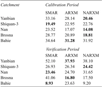
The r2 _{model component efficiency criterion, which}

was also suggested by Nash and Sutcliffe (1970), is used in the present study as a quantitative measure to assess the improvement in the performance of the NARXM

Table 1. Summary description of the test catchments.

Catchments Country Area Memory Calibration Verification Data Climate

km2 _{length period period starting}

(day) (years) (years) date

Yanbian China 2350 30 6 2 1 Jan. 1978 Humid

Shiquan-3 China 3092 15 6 2 1 Jan. 1973 Semi-arid

Nan Thailand 4609 20 6 3 1Apr. 1978 Humid

Brosna Ireland 1207 30 8 2 1 Jan. 1969 Temperate

Baihe China 61780 15 6 2 1 Jan. 1972 Semi-arid

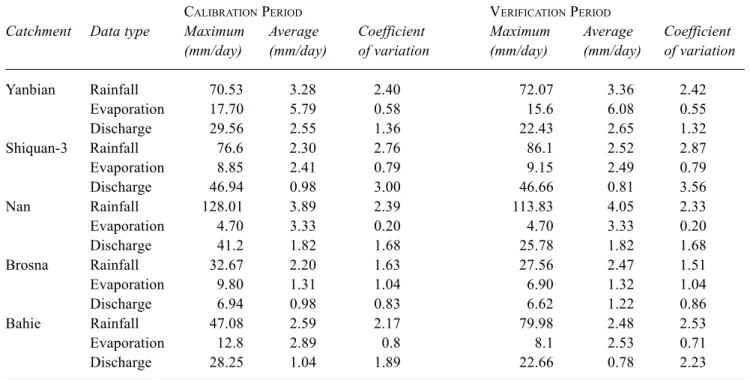
Table 2. Statistical summary of the Data of the test catchments

CALIBRATION PERIOD VERIFICATION PERIOD

Catchment Data type Maximum Average Coefficient Maximum Average Coefficient (mm/day) (mm/day) of variation (mm/day) (mm/day) of variation

Yanbian Rainfall 70.53 3.28 2.40 72.07 3.36 2.42 Evaporation 17.70 5.79 0.58 15.6 6.08 0.55 Discharge 29.56 2.55 1.36 22.43 2.65 1.32 Shiquan-3 Rainfall 76.6 2.30 2.76 86.1 2.52 2.87 Evaporation 8.85 2.41 0.79 9.15 2.49 0.79 Discharge 46.94 0.98 3.00 46.66 0.81 3.56 Nan Rainfall 128.01 3.89 2.39 113.83 4.05 2.33 Evaporation 4.70 3.33 0.20 4.70 3.33 0.20 Discharge 41.2 1.82 1.68 25.78 1.82 1.68 Brosna Rainfall 32.67 2.20 1.63 27.56 2.47 1.51 Evaporation 9.80 1.31 1.04 6.90 1.32 1.04 Discharge 6.94 0.98 0.83 6.62 1.22 0.86 Bahie Rainfall 47.08 2.59 2.17 79.98 2.48 2.53 Evaporation 12.8 2.89 0.8 8.1 2.53 0.71 Discharge 28.25 1.04 1.89 22.66 0.78 2.23

updating procedure over that of the corresponding ARXM updating. The r2 _{criterion, for the chosen}

lead-time, is calculated using the following equation:

2 ARXM 2 ARXM 2 NARXM 2 R -1 R -R = r (11) where 2 NARXM R and 2 ARXM

R are the corresponding R2 _values

of the NARXM and the ARXM updating procedures for the chosen lead-time, respectively. Negative values of r2 _{in the above equation signify that the performance}

of the NARXM updating procedure is worse than that of the ARXM updating procedure.

(2) The Average Relative Error (ARE) of the annual peak flow can be visualised as a rather crude measure of the

effectiveness of model peak discharge forecasts, this being an important issue in the context of real-time flood forecasting. The Relative Error (RE), for a given year, is defined as p p p p p Q Q Qˆ Q ∆Q RE= = − (12)

where Qˆ and _p Q are the model estimated andp

observed annual peaks, respectively, for that year. A value of RE of zero indicates perfect matching of the annual flood peak. A large value of RE would be an indication of the failure of the model to reproduce the annual peak. The average relative error (ARE) index is simply the average of the RE values for the relevant period (i.e. either the calibration or verification period).

As the selected measure of model error to be minimised in the calibration of the SMAR model is a weighted combination of the sum of squares of the forecasted discharge errors F and the corresponding index of volumetric fit, (i.e. a multiple objective function), the value of R2 _so

obtained is less than that for the case in which the volumetric error component of the objective function is neglected. However, this is not a primary consideration in the present study, in which the focus is on the updating procedures, as the same un-updated discharge series is used for both of the updating procedures tested. The choice of objective function ultimately adopted by the forecaster must naturally depend on the requirements of the forecast.

Similarly, indices other than the R2 _{and the ARE model}

efficiency indices considered above can reflect different characteristics of the forecasts, and the choice of indices to be adopted by the modeller depends on the objective of the study. For example, the forecast phase-error can be of critical importance in the context of real time forecasting, and the inclusion of a measure of the phase error would generally be appropriate in that context. As the SMAR model hydrographs for the catchments considered in the present study do not exhibit significant phase errors, it was felt that the ARE index, together with the R2 _{criterion are sufficient}

for the purposes of this study.

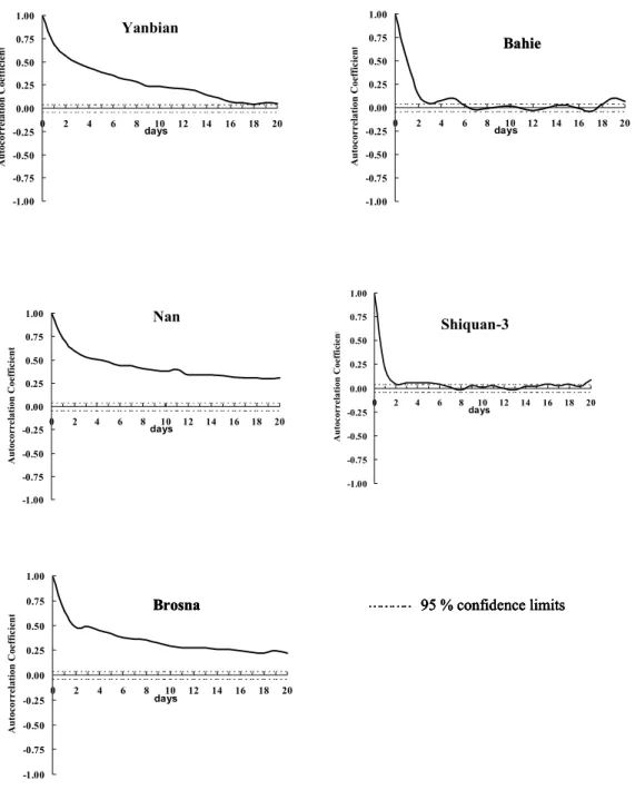
Figure 5 shows plots of the autocorrelation functions of the errors time series of the simulation mode estimated discharges of the SMAR model for the five catchments. Analysis of this figure indicates that, in the case of the three temperate and humid catchments, namely, Yanbian, Nan and Brosna, the corresponding error series tend to show a strong time persistence structure (i.e. substantial serial autocorrelations). However, in the case of the remaining two semi-arid catchments, namely, Shiquan-3 and Bahie, the autocorrelation in the error time series is weak. In these two semi-arid catchments, the autocorrelation coefficient values for non-zero lags are not significantly different from zero, except for lag times of one and two days.

The calibration of the ARXM updating involves the determination of the order (p) of the autoregressive part, the order (q) of the exogenous-input part and the corresponding parameter/coefficient values of the linear difference equation. Thus, the total number of parameters to be estimated in this updating procedure is N = (p+q+1). For chosen values of p and q, the optimum parameter values of the ARXM are estimated by the method of ordinary least squares. In the present study, an iterative process estimates the optimum values of p and q. In this iterative process, the ARXM is calibrated over a range of increasing values of p and q. The optimum values of p and q are those beyond which an increase in the values of these orders does not

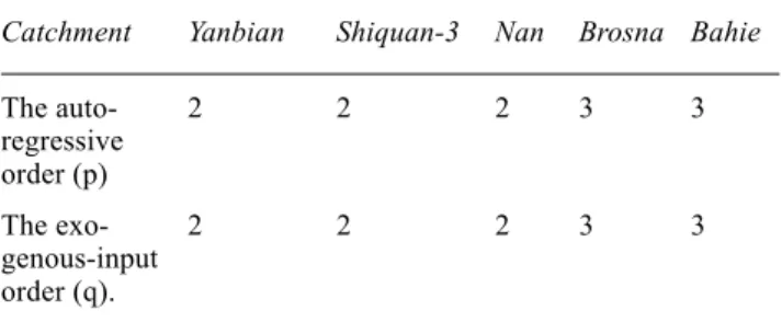
produce a significant increase in the overall efficiency of the ARXM updating procedure. This sequential calibration procedure generally yields a parsimonious model. Table 3 shows the optimum values of p and q for each of the five test catchments.

Similar to the ARXM updating procedure, the calibration of the NARXM updating procedure involves the determination of the (non-linear) auto-regressive order p and the (non-linear) exogenous input order q of Eqn.(4), the number of neurons in the single hidden layer and also the values of network parameters (i.e. the weights and the neuron threshold values). In general, the optimum values of p and q of the NARXM procedure can be estimated by an iterative procedure similar to that of the ARXM procedure, which is described previously. However, the optimum order values of the two updating procedures may differ. Various procedures for estimating the orders of the NARXM are discussed in Bomberger and Serborg (1998), Previdi et al. (1999) and Yu et al. (2000).

In the present study, for each catchment, the values of p and q of the NARXM updating procedure are taken to be the same as those of the corresponding ARXM updating procedure, so that both procedures use the same input information, thereby providing a fair basis for the comparison of their results. For specified values of p, q and the number of hidden neurons, the parameters of the NARXM updating model are estimated using the sequential optimisation procedure described below which minimises the sum of the squares of the differences between the network outputs and the re-scaled observed discharges values.

The parameter values of the NARXM are obtained using a computer program, developed by the present authors, for a sequential procedure involving two optimisation algorithms, namely, the genetic and the conjugate gradient algorithms. The genetic algorithm involves runs of ten thousand iterations and its set of parameter values giving the best results is used as the starting set for the conjugate gradient algorithm. Using the conjugate algorithm, the

Table 3. The autoregressive and the exogenous input moving

orders of the ARXM updating procedure.

Catchment Yanbian Shiquan-3 Nan Brosna Bahie

The auto- 2 2 2 3 3 regressive order (p) The exo- 2 2 2 3 3 genous-input order (q).

-1.00 -0.75 -0.50 -0.25 0.00 0.25 0.50 0.75 1.00 0 2 4 6 8 10 12 14 16 18 20 days Autocorrelation Coefficien t -1.00 -0.75 -0.50 -0.25 0.00 0.25 0.50 0.75 1.00 0 2 4 6 8 10 12 14 16 18 20 days Autocorrelation Coefficien t -1.00 -0.75 -0.50 -0.25 0.00 0.25 0.50 0.75 1.00 0 2 4 6 8 10 12 14 16 18 20 days Autocorrelation Coefficien t -1.00 -0.75 -0.50 -0.25 0.00 0.25 0.50 0.75 1.00 0 2 4 6 8 10 12 14 16 18 20 days Autocorrelation Coefficient -1.00 -0.75 -0.50 -0.25 0.00 0.25 0.50 0.75 1.00 0 2 4 6 8 10 12 14 16 18 20 days Autocorrelation Coefficien t Yanbian Bahie Brosna Nan _Shiquan-3 95 % confidence limits -1.00 -0.75 -0.50 -0.25 0.00 0.25 0.50 0.75 1.00 0 2 4 6 8 10 12 14 16 18 20 days Autocorrelation Coefficien t -1.00 -0.75 -0.50 -0.25 0.00 0.25 0.50 0.75 1.00 0 2 4 6 8 10 12 14 16 18 20 days Autocorrelation Coefficien t -1.00 -0.75 -0.50 -0.25 0.00 0.25 0.50 0.75 1.00 0 2 4 6 8 10 12 14 16 18 20 days Autocorrelation Coefficien t -1.00 -0.75 -0.50 -0.25 0.00 0.25 0.50 0.75 1.00 0 2 4 6 8 10 12 14 16 18 20 days Autocorrelation Coefficient -1.00 -0.75 -0.50 -0.25 0.00 0.25 0.50 0.75 1.00 0 2 4 6 8 10 12 14 16 18 20 days Autocorrelation Coefficien t Yanbian Bahie Brosna Nan _Shiquan-3 95 % confidence limits -1.00 -0.75 -0.50 -0.25 0.00 0.25 0.50 0.75 1.00 0 2 4 6 8 10 12 14 16 18 20 days Autocorrelation Coefficien t -1.00 -0.75 -0.50 -0.25 0.00 0.25 0.50 0.75 1.00 0 2 4 6 8 10 12 14 16 18 20 days Autocorrelation Coefficien t -1.00 -0.75 -0.50 -0.25 0.00 0.25 0.50 0.75 1.00 0 2 4 6 8 10 12 14 16 18 20 days Autocorrelation Coefficient -1.00 -0.75 -0.50 -0.25 0.00 0.25 0.50 0.75 1.00 0 2 4 6 8 10 12 14 16 18 20 days Autocorrelation Coefficien t Yanbian Bahie Brosna Nan _Shiquan-3 95 % confidence limits -1.00 -0.75 -0.50 -0.25 0.00 0.25 0.50 0.75 1.00 0 2 4 6 8 10 12 14 16 18 20 days Autocorrelation Coefficien t -1.00 -0.75 -0.50 -0.25 0.00 0.25 0.50 0.75 1.00 0 2 4 6 8 10 12 14 16 18 20 days Autocorrelation Coefficient -1.00 -0.75 -0.50 -0.25 0.00 0.25 0.50 0.75 1.00 0 2 4 6 8 10 12 14 16 18 20 days Autocorrelation Coefficien t Yanbian Bahie Brosna Nan _Shiquan-3 95 % confidence limits 95 % confidence limits

Fig. 5. Autocorrelation function of the SMAR model error time series

calibration process stops if one of the following three conditions is satisfied (Press et al., 1989, p. 305)

(i) The number of iterations exceeds five thousand (ii) The gradient of the objective function becomes zero

(i.e. the optimum value is obtained). This condition is unlikely in most cases.

(iii) The absolute difference between two successive values of the objective function is small, which is evaluated according to the inequality

where OF_i and OF_i+1 are the objective function values for iteration numbers i and i+1, respectively. In the present study, the number of iterations was always below the maximum number, with a range of variation between one hundred and one thousand. The same optimisation ‘stopping criteria’ were applied to all of the test catchments.

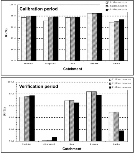
Figure 6 shows the R2 _{valuesof the NARXM updating}

procedure, for a lead-time of 1-day, for different numbers of hidden neurons ranging between two and four. Examination of this figure shows that, in both the calibration and verification periods, there is real improvement in the

) 10 ) ( ) ( ( 10 ) ( 2 10 1 10 1 − + − + + + × ≤ − × i i i i OF ABS OF ABS OF OF ABS

overall performance of the NARXM by increasing the number of the hidden neurons, from two to five, in the case of three out of the five test catchments, namely, Yanbian, Nan and Brosna. In the case of Bahie (one of the remaining two catchments), it is seen that while there is some improvement in the performance of the NARXM with the increase of the number of hidden neurons in the calibration period, the converse is true in the verification period. In the calibration period of Shiquan-3 (the other remaining catchment), there is significant improvement in the R2 _values

with the increase in the number of hidden neurons but, in the verification period, the R2 _{values for two and three hidden}

neurons are virtually the same, with just a slight increase in the R2 _{value when the number of neurons is increased to}

four. From the above discussion on Fig. 6, it can be argued that the appropriate number of the hidden neurons in the NARXM used for these catchments can be taken as two since this would generally yield R2 _{values that are either as}

good as or better in some cases than those obtained using more than two hidden neurons.

Table 4 shows the simulation-mode (un-updated) R2 _values

of the SMAR model for the five selected catchments. Likewise, Table 5 shows the R2 _{values of the ARXM and}

the NARXM updating procedures, for the same five catchments, for forecast lead times of one to four days. The table also displays the corresponding R2 _{values of the naïve}

persistence predictor-updating model (PPM) (i.e. the ‘no-rainfall-runoff-model’ situation), which postulates that the discharge forecast over the lead-time of any magnitude is simply equal to the observed discharge at the time of making the forecast. Note that this naïve updating model is used in the present study purely as a datum or baseline for comparing the performance of the more substantial ARXM and the NARXM updating procedures, since any serious real-time forecasting system should provide substantially better updated forecasts than the PPM.

Comparison of Tables 4 and 5 shows that updating the simulation mode discharges produced by the ARXM and the NARXM updating procedures has substantially improved the respective R2 _{values of the different lead-times,}

Fig. 6. Comparison of the lead-time of one-day R2 _{values of the NARXM updating procedure,}

in the calibration periods, for different numbers of hidden neurons

7 5 .0 8 0 .0 8 5 .0 9 0 .0 9 5 .0 1 0 0 .0 Y a n b ia n S h iq u a n -3 N a n B ro sn a B a ih e Catchment R 2(%) 2 hidden neurons 3 hidden neurons 4 hidden neurons 7 5 .0 8 0 .0 8 5 .0 9 0 .0 9 5 .0 1 0 0 .0 Y a n b ia n S h iq u a n -3 N a n B ro sn a B a ih e Catchment R 2(%) 2 hidden neurons 3 hidden neurons 4 hidden neurons Calibration period Verification period

for both the calibration and verification periods. For example, in the case of the Brosna catchment, the simulation mode efficiency in the calibration period is 85.87% while the corresponding R2 _{efficiency values for the ARXM and}

the NARXM for the forecast lead-time of 1-day are 95.02% and 96.08%, respectively. In most cases, the R2 _efficiency

values of the naïve PPM updating procedure are worse (i.e. lower) even than the simulation-mode (un-updated) efficiency values of the SMAR model. However, the case of the Brosna is an exception, having a PPM value of R2 ₌

87.86% for the one-day forecast lead time but this is still much lower than the corresponding R2 _{values given above}

for the ARXM and NARXM updating procedures. Examination of Table 5 reveals that both the NARXM and the ARXM updating procedures, operating on the

Table 4. Simulation mode R2 _{(%) efficiency values of the}

SMAR model.

Catchment Yanbian Shiquan-3 Nan Brosna Bahie

Efficiency 85.87 89.74 84.02 85.83 83.29 in the calibration period Efficiency 83.93 68.18 83.70 85.39 72.79 in the verification period

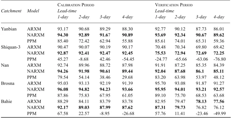
Table 5. The lead-time R2 _{(%) efficiency values of the ARXM, the NARXM and the PPM updating procedures.}

CALIBRATION PERIOD VERIFICATION PERIOD

Catchment Model Lead-time Lead-time

1-day 2-day 3-day 4-day 1-day 2-day 3-day 4-day

Yanbian ARXM 93.17 90.68 89.29 88.30 92.77 90.12 87.73 86.01 NARXM 94.30 92.89 91.67 90.89 93.69 92.34 90.67 89.62 PPM 85.40 72.42 62.94 55.88 85.61 74.01 65.31 59.36 Shiquan-3 ARXM 90.47 90.07 90.19 90.17 70.48 70.34 69.80 69.42 NARXM 92.87 92.41 92.47 92.45 75.53 72.94 72.69 72.25 PPM 45.27 -8.68 42.46 -54.45 -24.77 -65.66 -63.06 -76.80 Nan ARXM 92.74 89.96 88.72 87.98 91.91 87.25 85.35 84.39 NARXM 94.26 91.98 90.61 89.44 92.04 87.68 86.1 85.11 PPM 79.54 54.14 38.46 29.68 83.20 63.98 53.97 48.12 Brosna ARXM 95.03 93.13 92.19 91.39 95.70 93.08 91.87 91.27 NARXM 96.08 94.82 94.23 93.66 95.95 94.01 93.21 92.57 PPM 87.86 75.83 67.95 61.05 89.10 75.70 68.53 63.68 Bahie ARXM 88.29 84.11 83.79 83.78 82.95 79.47 78.13 77.56 NARXM 92.17 89.03 87.99 87.62 87.31 79.73 76.82 76.12 PPM 67.58 22.57 -8.95 -26.68 57.76 11.41 -23.46 -49.99

SMAR model simulation-mode forecasts, perform substantially better than the naïve PPM updating procedure. This table also shows that the NARXM updating procedure

has better R2 _{values than those of the ARXM updating}

procedure, for both the calibration and the verification periods, in the case of four catchments, namely, Yanbian, Shiquan-3, Nan and Brosna. However, in the case of the fifth catchment, namely, Baihe, the NARXM has better performance than the ARXM in the calibration period only. In the verification period of the Baihe catchment, the ARXM updating procedure has higher R2 _{values than the NARXM}

updating procedure for lead-times of three and four days. Furthermore, as expected, inspection of Table 5 shows that the lead-time R2 _{efficiency values of the updating}

procedures decrease with the increase in the value of the lead-time. In the case of the ARXM and the NARXM these lead-time efficiency values converge in the limit to the R2

efficiency value of the simulation mode forecast of the SMAR model. The time of such convergence varies from catchment to catchment, depending on the degree of persistence in the structure of the error series of the simulation mode forecasts of the SMAR model. In general, the convergence is faster in the case of the two semi-arid catchments.

Figure 7 shows scatter plots of the updated discharge forecasts of the ARXM and NARXM updating procedures in the calibration period, for a forecast lead-time of one day. An examination of these scatter plots indicates that in the