The edge of thermodynamics : driven steady states in physics and biology

(1)

The Edge of Thermodynamics:

Driven Steady States in Physics and Biology

by

Robert Alvin Marsland III

Submitted to the Department of Physics

in partial fulfillment of the requirements for the degree of

Doctor of Philosophy

at the

MASSACHUSETTS INSTITUTE OF TECHNOLOGY

June 2017

c

○ Massachusetts Institute of Technology 2017. All rights reserved.

Author . . . .

Department of Physics

May 24, 2017

Certified by . . . .

Jeremy L. England

Cabot Career Development Associate Professor of Physics

Thesis Supervisor

Accepted by . . . .

Nergis Mavalvala

Curtis and Kathleen Marble Professor of Astrophysics

Associate Department Head of Physics

(2)

(3)

The Edge of Thermodynamics:

Driven Steady States in Physics and Biology

by

Robert Alvin Marsland III

Submitted to the Department of Physics on May 24, 2017, in partial fulfillment of the

requirements for the degree of Doctor of Philosophy

Abstract

From its inception, statistical mechanics has aspired to become the link between bi-ology and physics. But classical statistical mechanics dealt primarily with systems in thermal equilibrium, where detailed balance forbids the directed motion characteris-tic of living things. Formal variational principles have recently been discovered for nonequilibrium systems that characterize their steady-state properties in terms of gen-eralized thermodynamic quantities. Concrete computations using these principles can usually only be carried out in certain limiting regimes, including the near-equilibrium regime of linear response theory. But the general results provide a solid starting point for defining these regimes, demarcating the extent to which system’s behavior can be understood in thermodynamic terms.

I use these new results to determine the range of validity of a variational proce-dure for predicting the properties of near-equilibrium steady states, illustrating my conclusions with a simulation of a sheared Brownian colloid. The variational principle provides a good prediction of the average shear stress at arbitrarily high shear rates, correctly capturing the phenomenon of shear thinning. I then present the findings of an experimental collaboration, involving a specific example of a nonequilibrium struc-ture used by living cells in the process of endocytosis. I first describe the mathematical model I developed to infer concentrations of signaling molecules that control the state of this structure from existing microscopy data. Then I show how I performed the inference, with special attention to the quantification of uncertainty, accounting for the possibility of “sloppy modes” in the high-dimensional parameter space. In the final chapter I identify a trade-off between the strength of this kind of structure and its speed of recovery from perturbations, and show how nonequilibrium driving forces can accelerate the dynamics without sacrificing mechanical integrity.

Thesis Supervisor: Jeremy L. England

(4)

(5)

Acknowledgments

This interdisciplinary work would not have been possible without the generous col-laboration of a large number of people with a wide range of expertise. First of all, I would like to thank Prof. Jeremy England for his mentorship over these past five years, and for nurturing such a vibrant intellectual environment in our lab. It has been wonderful to see the group grow and mature almost from its very beginnings, and I owe a great deal of my own personal growth during this time to its rich atmo-sphere of genuine friendship and serious scholarship. I am also grateful for the hard work of the administrative staff – especially to Catherine Modica, who has been so helpful and encouraging from the beginning of my degree to the end.

I need to express my deep appreciation for the hospitality of Prof. Tomas Kirch-hausen and his group, who have patiently brought me up to speed on some of the most exciting topics in cell biology, and transformed me from a physicist curious about bi-ology into a biophysicist. Special thanks go to Kangmin He, who welcomed me into his core postdoctoral project, and performed all the experiments that form the basis of my fourth chapter. I also had many valuable conversations with Ilja Kusters, Ben-jamin Capraro, Gokul Upadhyayula, and Joe Sarkis about scientific issues related to this project. I want to thank Catherine McDonald as well, for always being ready to help with any logistical issue.

I am grateful to Tal Kachman for introducing me to Python and the iPython Notebook. The numerical work and data analysis in Chapters 3 - 5 would have been much more challenging and time-consuming without these helpful tools. For the sim-ulations of Chapter 3, I want to acknowledge the contribution of Benjamin Harpt, an undergraduate research assistant who helped me finish that project and start explor-ing some possible extensions. The model of Chapter 5 matured through discussions with another undergraduate researcher, Arsen Vasilyan, and with postodoc Sumantra Sarkar.

Finally, I want to thank my friends who have generously given me feedback on this manuscript and related papers. Jordan Horowitz, Todd Gingrich, Gili Bisker and

(6)

Zachary Slepian have each dedicated time to reading and commenting on my drafts, and have dramatically improved the quality of the final product.

(7)

5.2.1 Transition Rates . . . 112 5.2.2 Mean-Field Interactions . . . 114 5.2.3 Coarse-Grained Rates . . . 116 5.3 Steady-State Solution . . . 117 5.3.1 Stationary State . . . 118 5.3.2 Dynamics . . . 122 5.3.3 Energetics . . . 124 5.4 Cost of Acceleration . . . 126 5.4.1 Results . . . 126 5.4.2 Discussion . . . 128 6 Conclusions 131 A Microscopic Reversibility in the Langevin Equation 143 A.1 Langevin Equation for Brownian Motion . . . 144

A.2 Colloid Simulation with Externally Imposed Flows . . . 146

(10)

C Perturbative Calculations of Work Statistics for Nonlinear

Macro-scopic Dynamics 155

C.1 Mathematical Preliminaries . . . 155

C.2 Driving by Imposed Flow . . . 158

C.3 Driving by Thermal/Chemical/Mechanical forces . . . 160

D Physical Justification of Mean Wall Stress 163 D.1 Stress in Newtonian Fluids . . . 164

D.2 Mapping to Electrostatics . . . 166

D.3 Obtaining the Induced Charge on the Conducting Plate . . . 167

D.3.1 Contribution of Variations about the Mean . . . 169

D.3.2 Contribution of the Mean Charge . . . 170

(11)

Chapter 1 Introduction

The general struggle for existence of animate beings is therefore not a struggle for raw materials - these, for organisms, are air, water and soil, all abundantly available - nor for energy which exists in plenty in any body in the form of heat (albeit unfortunately not transformable), but a struggle for entropy, which becomes available through the transition of energy from the hot sun to the cold earth.

– Ludwig Boltzmann, 1886 [10, p.24]

From the standpoint of statistical mechanics, as Boltzmann points out in this quotation, the characteristic activities of living things are part of the process by which the universe tends towards a state of maximum entropy. Schrödinger came back to this point in his lecture series What is Life? [89], and since then it has remained a constant theme in biophysics.

Both Boltzmann and Schrödinger place the connection to statistical mechanics in a “no-go theorem”: the activities of living things are impossible in thermal equi-librium, and necessarily depend on harnessing a pre-existing disequilibrium like the temperature difference between earth and sun. This is simply an extension of the most basic statement of the Second Law of Thermodynamics, which implies that engines can only run in an environment that has not yet reached its maximum en-tropy. Most successful applications of statistical physics to biology are quantitative

(12)

elaborations on this claim, investigating how much entropy is actually generated in particular biological activities such as sensing, DNA replication and reproduction [59, 73, 72, 58, 85, 76, 82, 23].

But classical statistical mechanics is also predictive. Given a closed physical system that has been left alone for a sufficiently long time, we can predict the most likely value of any observable quantity by maximizing the system’s entropy. Living things are clearly not in a state of maximum entropy, since they exist precisely as processes on the way to maximum entropy. But perhaps there is some other quantity that is maximized or minimized in a living system’s most likely state, and can be estimated from knowledge of the organism’s constituent parts. This hope has generated and continues to generate considerable excitement (cf. [80]). If such a principle could be found, it would go a long way to explaining the origin of life on earth, and would pave the way for a predictive physical theory of biology.

Advances in the theory of stochastic processes and in the foundations of thermo-dynamics have made it possible to write down formal variational principles charac-terizing the most probable state of any observable in a nonequilibrium system, and to express these principles in terms of generalized thermodynamic quantities [19, 36, 7]. But the quantities involved in these exact results lack any direct empirical meaning, and can in general be computed only if the equations of motion have already been solved [86, 7].

The real value of these theoretical advances lies in their power to clarify the limits of thermodynamic reasoning [68]. For driven systems near equilibrium, considerations of work, energy and entropy lead to definite predictions of wide applicability such as the Einstein relation and more general fluctuation-dissipation theorems [21, 66]. These theorems are usually derived in the limit of vanishing nonequilibrium driving force, and the factors that determine their range of validity at finite driving force remain only vaguely specified. The new exact results for arbitrary driving now provide the necessary tools for defining this boundary. Knowing the boundary will not only steer us away from dead ends in our pursuit of biological understanding, but also help us mine all of the relevant insight from “near-equilibrium” results.

(13)

This thesis is a tour of the edge of thermodynamics. It is organized around two poles: a general theoretical result I derived concerning the range of linear response theory, and a set of experimental results I obtained in collaboration with the Kirch-hausen Laboratory at Harvard Medical School. In the final chapter, I bring these poles together by investigating the thermodynamic properties of the experimental system through the lens of a simplified stochastic model.

I begin Chapter 2 with a simple example: a piston of gas kept out of equilibrium by an oscillatory driving force. I use this example to illustrate a result from linear response theory, which shows how the probability of a fluctuation is controlled by its free energy minus the average work done by a nonequilibrium driving force on the way there. I then derive a general fluctuation theory for nonequilibrium steady states in terms of work statistics. Finally, I construct a novel perturbative analysis of this general formula that contains the linear response result as a limiting case, and provides a framework for determining precisely where and why it breaks down.

As becomes clear in the course of the derivation, the distinction between my analysis and the traditional linear response approach appears when the relaxation time of the system to its stationary state depends on the strength of the driving force. In my driven piston example, it is hard to identify a simple mechanism by which the amplitude of the pressure fluctuations could affect the rate of relaxation. But in many physical systems – especially systems of interacting particles – driving forces can “stir” the particle configuration and thereby accelerate the relaxation dynamics. In Chapter 3, I apply the theory of Chapter 2 to a concrete example of such a system, showing how the nonlinear response remains well-described by my near-equilibrium approximation.

Chapter 4 contains the results of my experimental collaboration. I start by intro-ducing the biological process I studied, focusing on the features of particular physical interest. This system involves a self-assembled structure that is switched “on” and “off” by modulation of the coupling to a nonequilibrium environment. The structure has to be switched off at a certain stage in the process, and for the past decade my collaborators have been advancing an interesting hypothesis about how this timing is

(14)

regulated. I translated this hypothesis into a quantitative model, and combined the model with some new data from their laboratory to assess its physical plausibility.

In Chapter 5, I use a model inspired by the biological system of Chapter 4 to illus-trate the novel material properties that become possible in a nonequilibrium steady state. The presence of an “active” disassembly pathway powered by an externally supplied free energy source allows mechanically robust structures to rapidly recover from large perturbations, something difficult to achieve in a passive material.

The thesis finishes with Chapter 6, where I sum up the conclusions of these four chapters, and point out what I believe to be the most promising future directions.

(15)

Chapter 2 The Edge of Linear Response

2.1 Introduction: A Driven Ideal Gas

Consider the cylinder depicted in Figure 2-1. It is filled with a dilute gas of 𝑁 particles, and immersed in an environment of uniform temperature 𝑇 and pressure 𝑃ext = 𝑃0. One wall of the cylinder is formed by a movable piston, so that the volume

is free to vary, and eventually relaxes to its equilibrium value 𝑉 = 𝑉0.

In thermal equilibrium, one can compute 𝑉0 in terms of the other parameters by

maximizing the entropy 𝑆tot of the whole setup – including the environment – which

is equal to minus the Gibbs free energy 𝐺 (up to an additive constant). At fixed temperature, the internal energy of an ideal gas is constant, as is the contribution to the system entropy from the momentum degrees of freedom, so 𝐺 is determined by the configurational entropy 𝑁 𝑘𝐵ln 𝑉 :

𝐺 = 𝐸 _{− 𝑇 𝑆 + 𝑃 𝑉 = −𝑘}𝐵𝑇 𝑁 ln 𝑉 + 𝑃0𝑉 + 𝑔(𝑇 ) (2.1)

where 𝑔(𝑇 ) is a function independent of 𝑉 . The Gibbs free energy is extremized at

0 = 𝜕𝐺 𝜕𝑉 =−

𝑘𝐵𝑇 𝑁

𝑉0

(16)

T

V

P

ext

V

eq

V

ss

0 2⇡/!

4⇡/!

P (t)

V (t)

t

V (t)

V

eq

V

ss

G(V )

Figure 2-1: Color. Top left: Cylinder filled with 𝑁 non-interacting particles. The volume 𝑉 available to the gas varies in response to changes in an externally controlled pressure 𝑃ext applied to the movable piston on the right side of the container. The

cylinder is immersed in an equilibrated environment of temperature 𝑇 and pressure 𝑃ext = 𝑃0. Top right: Adding a small periodic perturbation ∆𝑃 (𝑡) = ∆𝑃0sin(𝜔𝑡) to

the original constant pressure 𝑃ext = 𝑃0 drives the system away from its equilibrium

volume 𝑉eq = 𝑉0. I define a “steady state” by measuring the volume at discrete

time intervals separated by the driving period 2𝜋/𝜔. Bottom left: The equilibrium volume 𝑉eq can be found by minimizing the Gibbs free energy 𝐺(𝑉 ). The

steady-state volume 𝑉ss minimizes 𝒢 = 𝐺 − 𝑊 , where 𝑊 (𝑉 ) is the typical work done by the

periodic perturbation ∆𝑃 during the fluctuation to volume 𝑉 . Bottom right: The typical trajectory to generate a given volume fluctuation away from the steady state for this linear system (top set of solid lines) is the sum of an exponential part that is independent of the drive properties (bottom set of solid lines), and a sinusoidal part that is independent of the size of the fluctuation (dotted line).

(17)

which agrees with the prediction of the ideal gas law 𝑉0 = 𝑁 𝑘𝐵𝑇 𝑃0 . (2.3)

2.1.1 Overdamped Model

The goal of this chapter is to determine the regime of validity of a generalization of this variational procedure for driven systems, which has traditionally been derived in linear response theory using the limit of vanishing driving force. I introduce the key concepts in this section by explicitly computing the steady-state volume 𝑉ss in a

model of a driven dilute gas, and showing that the linear response result leads to the same answer.

I drive the gas out of equilibrium by causing the external pressure 𝑃ext to vary in

time. The response of the volume will depend on the details of the system dynamics. I consider the case where friction between the piston and the cylinder is strong enough that the inertia of the piston is negligible, so the rate of change of volume is simply proportional to the pressure difference across the piston:

𝑑𝑉 𝑑𝑡 =−𝛾 [︂ 𝑃ext(𝑡)− 𝑁 𝑘𝐵𝑇 𝑉 ]︂ (2.4)

where 𝛾 is a friction coefficient that controls the timescale of relaxation.

For small enough variations of 𝑃ext = ∆𝑃 (𝑡) + 𝑃0 about 𝑃0, the volume change

∆𝑉 = 𝑉_−𝑉0 from the equilibrium volume at 𝑃0 will be much smaller than 𝑉0. In this

regime, the right-hand side can be approximated by the first two terms of a Taylor expansion in ∆𝑉 : 𝑑 𝑑𝑡∆𝑉 =−𝛾 [︂ 𝑃ext(𝑡)− 𝑁 𝑘𝐵𝑇 𝑉0 (︂ 1₋ 1 𝑉0 ∆𝑉 )︂]︂ (2.5) =_−𝛾𝑃0 (︂ ∆𝑃 (𝑡) 𝑃0 +∆𝑉 𝑉0 )︂ (2.6) =₋𝑉0 𝜏 (︂ ∆𝑃 (𝑡) 𝑃0 + ∆𝑉 𝑉0 )︂ (2.7)

(18)

where 𝜏 = 𝑉0/(𝑃0𝛾) is the relaxation timescale governing the exponential decay of

∆𝑉 to its equilibrium state at fixed ∆𝑃 near 𝑃0.

2.1.2 Periodic Steady State

The homogeneous solution of Equation (2.7), for ∆𝑃 = 0, can be read off immediately:

∆𝑉 = ∆𝑉0𝑒−𝑡/𝜏 (2.8)

For a sinusoidal driving force ∆𝑃 (𝑡) = ∆𝑃0sin 𝜔𝑡, the particular solution is

∆𝑉 (𝑡) = ₋_√ 𝑉0 1 + 𝜔2_𝜏2

∆𝑃0

𝑃0

sin(𝜔𝑡_{− 𝜑)} (2.9)

where the phase shift is 𝜑 = tan−1𝜔𝜏 .

The general solution for an arbitrary initial condition can be written as the sum of the particular solution and a scaled copy of the homogeneous solution:

∆𝑉 (𝑡) =₋_√ 𝑉0 1 + 𝜔2_𝜏2

∆𝑃0

𝑃0

sin(𝜔𝑡_{− 𝜑) + 𝛿𝑉 𝑒}−𝑡/𝜏 (2.10) where the constant 𝛿𝑉 controls the initial volume.

The periodic driving prevents ∆𝑉 from relaxing to any fixed value. To define a stationary state, I observe the system stroboscopically, taking snapshots at discrete times 𝑡𝑛 = 2𝜋_𝜔𝑛 with 𝑛 = 0, 1, 2, 3 . . . . These are the times when the pressure returns

to 𝑃0 from below. This choice implies sin(𝜔𝑡𝑛− 𝜑) = − sin 𝜑 = −𝜔𝜏/

√

1 + 𝜔2_𝜏2 _for

all 𝑛, so that the distance from the equilibrium volume 𝑉0 at observation time 𝑡𝑛 is

given by: ∆𝑉 (𝑡𝑛) = 𝑉0 𝜔𝜏 1 + 𝜔2_𝜏2 ∆𝑃0 𝑃0 + 𝛿𝑉 𝑒−𝑡𝑛/𝜏_. _(2.11)

In the limit 𝑡𝑛 → ∞, these stroboscopic measurements relax to a stationary value:

∆𝑉ss = 𝑉0 𝜔𝜏 1 + 𝜔2_𝜏2 ∆𝑃0 𝑃0 . (2.12)

(19)

This is the steady-state volume I set out to compute, given in terms of the nonequi-librium drive parameters 𝜔 and ∆𝑃0.

2.1.3 A Variational Principle

I will now obtain the same answer from a thermodynamic perspective.

The physical intuition for generalizing free energy minimization is most accessible in the context of fluctuation theory. While I began by considering a macroscopic system whose dynamics are effectively deterministic, a finite thermal system is neces-sarily subject to fluctuations. The probability 𝑝eq(𝑉 ) of a given fluctuation away from

the deterministic volume 𝑉* in a large system at thermal equilibrium is determined by the decrease in entropy ∆𝑆tot = 𝑆tot(𝑉 )− 𝑆tot(𝑉*):

𝑝eq(𝑉 )∝ 𝑒Δ𝑆tot(𝑉 )/𝑘𝐵 ∝ 𝑒−Δ𝐺(𝑉 )/𝑘𝐵𝑇 (2.13)

where 𝑆tot is the entropy of the whole setup, and 𝐺(𝑉 ) is the Gibbs free energy of

the ideal gas, as defined in Equation (2.1). This relationship is essentially a coarse-grained version of the Boltzmann distribution. It was first identified by Einstein [22] and has since been confirmed more rigorously in the large system size limit, using the methods of large deviation theory [95].

In 1959, James McLennan showed that the correction to the Boltzmann distribu-tion for near-equilibrium steady states is related in a simple way to the work done by the external driving forces [71, 65]. The coarse-grained version of his finding gives:

𝑝ss(𝑉 )∝ 𝑒−[Δ𝐺(𝑉 )−𝑊ex(𝑉 )]/𝑘𝐵𝑇 (2.14)

where 𝑊ex(𝑉 ) = 𝑊 (𝑉 )− 𝑊 (𝑉*) is the “excess work” done on the way to the

fluc-tuation. For my driven piston, 𝑊 (𝑉 ) is the work done by the pressure perturbation ∆𝑃 (𝑡) over a trajectory of duration _{𝒯 ≫ 𝜏 that ends in a state with volume 𝑉 .}

(20)

quantity

𝒢(𝑉 ) = 𝐺(𝑉 ) − 𝑊 (𝑉 ). (2.15)

Evaluating the work on the way to a fluctuation 𝑊 (𝑉 ) requires knowing the most likely trajectory that leads to the fluctuation. Detailed balance requires that the most likely fluctuation trajectories in thermal equilibrium are mirror images of the corresponding relaxation trajectories. In this linearized nonequilibrium model, the homogeneous part of the fluctuation trajectory (which is the solution in the absence of a driving force) will thus be the mirror image of the homogeneous part of the relaxation trajectory. Since only the homogeneous part of the solution depends on the initial condition ∆𝑉 , the mean work done on the way to a fluctuation is given by

𝑊 (∆𝑉 ) = ∫︁ 0 −∞ ∆𝑃 (𝑡) ˙𝑉 𝑑𝑡 (2.16) = 1 𝜏 ∫︁ 0 −∞ ∆𝑃0sin(𝜔𝑡)∆𝑉 𝑒𝑡/𝜏 + const. (2.17) = ∆𝑃0∆𝑉 𝜔𝜏 1 + 𝜔2_𝜏2 + const. (2.18)

where I have suppressed constant terms that are independent of ∆𝑉 . The steady-state volume is now found by minimizing

𝒢 = 𝐺 − 𝑊 = 𝑃0𝑉0 2 (︂ ∆𝑉 𝑉0 )︂2 − ∆𝑃0∆𝑉 𝜔𝜏 1 + 𝜔2_𝜏2 + const., (2.19)

where I have approximated the free energy 𝐺 by the lowest-order non-vanishing term in a Taylor expansion about 𝑉0. This new quantity is minimized when

0 = 𝜕𝒢 𝜕𝑉 = 𝑃0 𝑉0 ∆𝑉 _{− ∆𝑃}0 𝜔𝜏 1 + 𝜔2_𝜏2. (2.20)

Solving for ∆𝑉 yields the steady-state volume difference

∆𝑉ss = 𝑉0 𝜔𝜏 1 + 𝜔2_𝜏2 ∆𝑃0 𝑃0 . (2.21)

(21)

This agrees with the direct calculation of Equation (2.12), in accord with McLennan’s general result (2.14).

2.1.4 Range of Validity

I performed the above derivation in the ∆𝑃0 → 0 limit, following the standard

ap-proach of linear response theory. But Equation (2.21) can remain valid far from this limit, depending on the size of 𝜏 relative to 1/𝜔. Figure 2-2 compares the prediction of Equation (2.21) with the actual steady-state value of ∆𝑉 (measured at observation times 𝑡𝑛 = 2𝜋_𝜔𝑛) from the full nonlinear equation (2.4). At small 𝜏 , the two values

show good agreement even when ∆𝑃0 is large enough to make the gas expand more

than ten times its original volume at the top of the drive cycle and the dynamics are clearly nonlinear.

The reason for this is shown in the bottom-left panel of Figure 2-2. The state at time 𝑡𝑛 is fully determined by the portion of the ∆𝑃 (𝑡) protocol contained in the

preceding time interval of order 𝜏 . As 𝜏 decreases, the system loses memory of its past states more quickly. When 𝜏 is sufficiently small, the nonlinear regions of the trajectory with large ∆𝑃 (𝑡)/𝑃0 can no longer have any effect on the state of the

system at the observation times 𝑡𝑛 (where ∆𝑃 = 0), and so the linearized results can

still provide an adequate prediction. If 𝜏 were somehow coupled to ∆𝑃0 as described

in the top right panel of Figure 2-2, so that 𝜏 asymptotically decreased as 1/∆𝑃0,

the “linear response” result (2.14) would predict the full nonlinear response of ∆𝑉ss

to ∆𝑃0 for arbitrarily large values of the forcing ∆𝑃0. It is hard to envision such a

mechanism in the driven piston, but the sheared suspension I will analyze in Chapter 3 has this behavior naturally built in to the dynamics.

The fluctuation theory of (2.14) also points the way towards a thermodynamic version of this analysis, which can be more readily generalized. Since Equation (2.14) is exact for when the dynamics are linear, it should start to fail only when nonlineari-ties significantly affect the amount of work done during the time 𝜏 immediately before the end of the trajectory. Since 𝑊ex(𝑉 ) appears in the exponent of (2.14) divided by

(22)

P

0

/P

0

V

/V

0 0.01 0 _0.4 _0.8 0.005 0.015

!t

0.98 0.02 0.04 1.02 0.06

Transient

Steady State

0.94 0.00

!⌧

V

/V

0

V

ss

V

_ss(0) 0.02 0.01 0.03 0.02 0.03 0.01 0

!t/2⇡

1 2 3 0 4 8 12

V

/V

0 ⌧ = ⌧0 1 + k P0/P0

V

/V

0

Figure 2-2: Top left: Steady-state volume difference ∆𝑉ss vs. relaxation time 𝜏 for

∆𝑃0 = 𝑃0. The near-equilibrium prediction 𝑉 (0)

ss from Equation (2.21) agrees well

with the exact solution 𝑉ss up to about 𝜔𝜏 ∼ 0.01. Top right: Nonlinear response

for imaginary scenario where 𝜏 depends on ∆𝑃0. If 𝜏 decreases asymptotically as

1/∆𝑃0, then the near-equilibrium result can remain valid for arbitrarily large choices

of ∆𝑃0. Bottom right: 𝑉 (𝑡) in the periodic steady state with this large ∆𝑃0 value

and 𝜔𝜏 = 0.01. The sinusoidal pressure changes produce a volume response with a very different shape, due to the nonlinearity of the dynamical equation (2.4). Bottom left: Zoomed-in plot of 𝑉 (𝑡) showing the relaxation dynamics to the periodic steady state. The system loses memory of its initial condition well before it leaves the region where the small-∆𝑉 approximation is valid.

(23)

𝑊ex(𝑉 ) during a typical fluctuation becomes comparable to 𝑘𝐵𝑇 . The limit of

vanish-ing drivvanish-ing force guarantees that this contribution is small, but Figure 2-2 indicates that this assumption is by no means necessary. The factor determining the validity of “near-equilibrium” results like (2.14) appears not to be the strength of the driv-ing, but the strength of nonlinearities measured in these thermodynamic terms. Over the course of this chapter, I will employ the tools of contemporary nonequilibrium statistical mechanics to confirm this conjecture for a broad class of systems.

2.2 Theoretical Framework

Almost 60 years after the publication of McLennan’s result, we are finally in a po-sition to see where it comes from, and thereby determine its full range of validity. This is primarily due to the conceptual reorganization of nonequilibrium statistical mechanics that has taken place over the past two decades, which highlights the role of time-reversal symmetry as the central physical principle of the theory [17, 47]. In this section I summarize this new way of looking at things, setting up the derivations of Section 2.4 where I obtain the conditions of validity for McLennan’s variational principle. All the important claims in this background section are standard results in the stochastic thermodynamics literature, but arranged and described in an orig-inal way. My novel results are contained in Sections 2.4-2.6, where I determine the boundaries of the near-equilibrium regime with a novel expansion in the degree of nonlinearity.

2.2.1 Microscopic Reversibility

The foundation of this new point of view on nonequilibrium statistical mechanics is the insight that statistical irreversibility enters time-symmetric dynamics via the distribution over environmental initial conditions. In this subsection I will present the core equation that captures this insight (2.24), after setting up the basic concepts required to write it down.

(24)

is described by a set of 𝑁 coordinates 𝑞𝑖 with conjugate momenta 𝑝𝑖. The dynamics

are given by Hamilton’s equations

˙ 𝑞𝑖 = 𝜕𝐻tot 𝜕𝑝𝑖 (2.22) ˙ 𝑝𝑖 =− 𝜕𝐻tot 𝜕𝑞𝑖 .

These equations of motion are deterministic, and symmetric under the time reversal operation 𝑡 _{→ −𝑡, 𝑝}𝑖 → −𝑝𝑖 (and also B → −B in the presence of a magnetic field

B). Any trajectory allowed by these equations of motion is therefore also allowed to happen in reverse. As illustrated in Figure 2-3, I will keep track of some subset of the degrees of freedom, which I will call the “system” and denote by x, and refer to the rest of the degrees of freedom y as the “environment.” The Hamiltonian can now be split into three parts: one that depends on the system degrees of freedom alone, one that depends on the environment alone, and one that couples the two sets together:

𝐻tot(x, y, 𝑡) = 𝐻sys(x, 𝜆𝑡) + 𝐻env(y) + ℎint(x, y) (2.23)

Importantly, I have allowed for an explicit time-dependence in the system Hamiltonian 𝐻sys (but not in the other terms) via a control parameter 𝜆𝑡. This generalizes the

extra external pressure ∆𝑃 (𝑡) from my introductory example, and can be used to do work on the system.

If I now choose the initial condition y0 of the environment at random, the

tra-jectory of the system degrees of freedom x from a given initial condition x0 becomes

stochastic. I will write the probability that x takes a given trajectory from this ini-tial condition as 𝑝[x𝒯₀_|x0, 𝜆𝒯0]. The symbol x

𝒯

0 denotes the whole trajectory from its

beginning at time 𝑡 = 0 to some chosen end time _{𝒯 . I have also explicitly included} the dependence on the variation of the control parameter 𝜆𝑡, using 𝜆𝒯0 to represent

its trajectory over the observation time. Rigorously defining this probability requires providing a suitable measure on the infinite-dimensional space of trajectories x𝒯₀. This is easy to do in the present context, since the trajectory x𝒯₀ from a given system initial

(25)

x

y

t

T

(1)

,

_{µ

(1)_i

_}

T

(2)

,

_{µ

(2)_i

_}

T

(3)

,{

µ

(3) i

}

T

(4)

,{

µ

(4) i

}

Figure 2-3: Color. Left: The 𝑁 degrees of freedom in a piece of isolated matter are partitioned into two sets, a system with microstate x and an environment with microstate y. The system is illustrated here as discrete particles, since I keep track of the full trajectories x𝒯₀. The environment is just a solid color, because I integrate it out to obtain an effective stochastic dynamics for x. Work can be done on the system by externally imposed variations in a set of parameters 𝜆, which affect only the system part of the Hamiltonian 𝐻sys. Right: I will focus on situations where the

environment can be modeled as a set of ideal thermal and chemical reservoirs with temperatures 𝑇(𝛼) and chemical potentials 𝜇(𝛼)_𝑖 .

(26)

condition x0 is fully determined by the environment state y0. The path measure can

thus be taken as the ordinary Liouville measure Π𝑖𝑑𝑝𝑖𝑑𝑞𝑖 on the environment phase

space.

This random choice of environment state can break time-reversal symmetry, intro-ducing statistical irreversibility into the effective stochastic dynamics. To measure the extent to which this symmetry is broken, we can compare the probability 𝑝[x𝒯₀_|x0, 𝜆𝒯0]

with the probability of the reverse trajectory 𝑝[ˆx𝒯₀_|x*_𝒯, ˆ𝜆𝒯₀]. I have introduced a new symbol ˆx𝒯₀ to denote the time-reversed version of x𝒯₀: the order in which the states are visited is reversed, and the signs of all the momenta are flipped. Similarly, ˆ𝜆𝒯₀ in-dicates the time-reverse of the control protocol 𝜆𝒯₀. If any magnetic fields are present, they are automatically included among the parameters 𝜆, and their signs are reversed in the reverse protocol. An individual state whose momenta have been reversed and a single set of control parameters with magnetic fields reversed are denoted by x* and 𝜆*, respectively.

If y0 is chosen from an equilibrium distribution over environment states, it turns

out that the statistical irreversibility of a given system trajectory x𝒯₀ is given by the change in the entropy of the environment ∆𝑆𝑒 over the course of the trajectory:

𝑝[ˆx𝒯₀_|x*_𝒯, ˆ𝜆𝒯₀] 𝑝[x𝒯₀_|x0, 𝜆𝒯0]

= 𝑒−Δ𝑆𝑒/𝑘𝐵_. _(2.24)

As I explain below, Equation 2.24 can be taken as a basic statement of the requirement of consistency between a asymmetric coarse-grained dynamics and the time-reversal symmetry of the fundamental dynamics. For this reason, it is often referred to in the literature as the “microscopic reversibility relation” [17]. It can also be viewed as a generalization of the requirement of detailed balance, and is sometimes called “local detailed balance” (cf. [91]). An analogous relation holds for quantum systems, thanks to the time-reversal symmetry of the Schrödinger equation [40].

(27)

2.2.2 Microcanonical Derivation

I will now examine the connection between Equation (2.24) and time-reversal symme-try in the Hamiltonian framework I have just described. I will deviate from standard derivations of this result, which initialize the environment in a canonical ensemble [45, 53], because this connection is clearer when the initial energy of the whole setup is fixed. In the limit of infinite environment size, my microcanonical approach gives the same answer as the older literature, confirming that the usual “equivalence of ensembles” in the thermodynamic limit remains valid in this context.

The whole setup including the environment and the system begins at time 𝑡 = 0 with total energy 𝐸. If the system begins in state x0, then the energy available to

the environment is 𝐸 _{− 𝐻}sys(x0, 𝜆0). I will denote the phase space volume occupied

by environment states y with this energy as Ω(𝐸 _{− 𝐻}sys(x0, 𝜆0)). To compute the

probability 𝑝[x𝒯₀_|x0, 𝜆𝒯0] of observing a given system trajectory x 𝒯

0, I count how many

of these allowed environment states give rise to x𝒯₀ under the equations of motion (2.22), when combined with the system initial condition x0 and the control protocol

𝜆𝒯₀. I denote the phase space volume occupied by these states as Ω[x𝒯₀_|x0, 𝜆𝒯0]. Now I

choose the initial environment state from a uniform distribution over the energetically allowed states contained in Ω(𝐸 _{− 𝐻}sys(x0, 𝜆0)). As illustrated in Figure 2-4, the

probability of choosing one of the states that produces the desired trajectory is:

𝑝[x𝒯₀_|x0, 𝜆𝒯0] =

Ω[x𝒯₀_|x0, 𝜆𝒯0]

Ω(𝐸_{− 𝐻}sys(x0, 𝜆0))

. (2.25)

The energy of the environment changes over the course of the trajectory, as heat flows in and out of the system. At the end of the trajectory, it is equal to 𝐸 + 𝑊 ₋ 𝐻sys(x𝒯, 𝜆𝒯), where the work 𝑊 done by manipulation of 𝜆 is

𝑊 = ∫︁ 𝒯 0 𝜕𝐻sys(x𝑡, 𝜆𝑡) 𝜕𝜆 ˙ 𝜆𝑡𝑑𝑡. (2.26)

Because the control parameter has a direct effect only on the system, and not on the environment, 𝑊 is fully determined by the protocol 𝜆𝒯₀ and the system trajectory x𝒯₀,

(28)

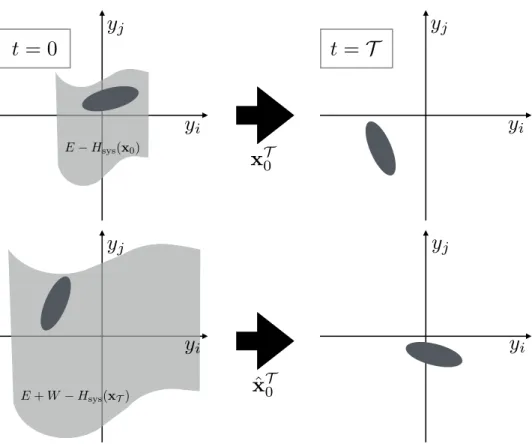
t = 0

t =

_T

x

T₀

ˆ

x

T₀

y

i

y

j

y

i

y

j

y

i

y

j

y

i

y

j E Hsys(x0) E + W Hsys(xT)

Figure 2-4: Top: Given an initial system state x0, at time 𝑡 = 0, the trajectory x𝒯0

is determined by the choice of initial environment state y0. If y0 is chosen from a

uniform distribution over a constant energy surface, the probability of choosing a state that generates a given x𝒯₀ is the ratio of the phase space volume occupied by these states (dark shaded region) to the total phase space volume available (light shaded region). Phase space volume is conserved by the Hamiltonian dynamics, and so the dark shaded region at time 𝑡 = 0 evolves into a new region at time 𝑡 = _𝒯 with the same volume but a new energy. Bottom: Reversing the momenta of the dark shaded region from the 𝑡 = _{𝒯 snapshot generates the initial conditions for the} reverse trajectory ˆx𝒯₀. The probability of observing this trajectory is again given by the ratio of this region’s volume to the volume of the entire set of environment states that share the same energy. The fact that both dark shaded regions occupy the same volume is a geometric statement of time-reversal symmetry, expressed symbolically in Equation (2.28).

(29)

regardless of what happens in the environment.

If I reverse the momenta, choose the environment conditions from this new energy surface, and run the protocol 𝜆𝑡 in reverse, then the probability of observing ˆx𝒯0 is

given by: 𝑝[ˆx𝒯₀_|x*_𝒯, ˆ𝜆𝒯₀] = Ω[ˆx 𝒯 0|x * 𝒯, ˆ𝜆𝒯0] Ω(𝐸 + 𝑊 _{− 𝐻}sys(x𝒯, 𝜆𝒯)) . (2.27)

Figure (2-4) shows how the numerators of Equations (2.25) and (2.27) are related by time-reversal symmetry:

Ω[ˆx𝒯₀_|x*_𝒯, ˆ𝜆₀𝒯] = Ω[x𝒯₀_|x0, 𝜆𝒯0], (2.28)

as long as Ω[x𝒯₀_|x0, 𝜆𝒯0] is evaluated using a measure that is invariant under the

system equations of motion (which is true of the usual Liouville measure 𝑑𝑝 𝑑𝑞). When combined with Boltzmann’s formula 𝑆 = 𝑘𝐵ln Ω, this way of expressing the

symmetry immediately leads to the desired result: 𝑝[ˆx𝒯₀_|x*_𝒯, ˆ𝜆𝒯₀] 𝑝[x𝒯₀_|x0, 𝜆𝒯0] = Ω(𝐸− 𝐻sys(x0, 𝜆0)) Ω(𝐸 + 𝑊 _{− 𝐻}sys(x𝒯, 𝜆𝒯)) = 𝑒−Δ𝑆𝑒/𝑘𝐵_. _(2.29)

2.2.3 Environment Entropy

The microcanonical definition of temperature _𝑇1 = 𝛽 = 𝜕𝑆𝑒

𝜕𝐸 implies that

∆𝑆𝑒[x𝒯0] = 𝛽∆𝑄[x 𝒯

0], (2.30)

where the heat ∆𝑄[x𝒯₀] = ∆𝐻tot− ∆𝐻sys is the change in the energy associated with

the environment degrees of freedom y when the system executes the trajectory x𝒯₀. As illustrated in Figure 2-3, more complex environments can be modeled with several ideal thermal and chemical reservoirs (indexed by 𝛼) at temperatures 𝑇(𝛼)_,

and chemical potentials 𝜇(𝛼)_𝑗 = _−𝑇(𝛼) 𝜕𝑆𝑒(𝛼)

𝜕𝑛(𝛼)_𝑗 , where 𝑛 (𝛼)

𝑗 is the number of particles

of type 𝑗 in reservoir 𝛼. My derivation can be generalized to handle this broader class of environments if each of the reservoirs is separately initialized in a uniform

(30)

distribution over states of fixed energy and particle number, and is coupled to the system at the beginning of the forward trajectory. The derivation from the canonical ensemble in [53] includes the possibility of particle exchange and multiple reservoirs from the beginning.

Now the system can be driven out of equilibrium without any time-variation in 𝜆, carrying fluxes of energy and matter from one reservoir to another. The entropy change in the environment becomes (cf. [81]):

∆𝑆𝑒(x𝒯0) = ∑︁ 𝛼 𝛽(𝛼) (︃ ∆𝑄(𝛼)[x𝒯₀]₋∑︁ 𝑗 𝜇(𝛼)_𝑗 ∆𝑛(𝛼)_𝑗 [x𝒯₀] )︃ . (2.31)

Throughout this chapter, I will make an analogy between systems driven by ex-ternal forces and those driven by thermal/chemical gradients, defining a generalized work _{𝒲 and an arbitrary reference temperature 𝑇 that restore the form of the First} Law for isothermal systems:

𝑇 ∆𝑆𝑒 =𝒲 − ∆𝐻sys (2.32) where 𝒲 ≡ 𝑊 + 𝑇 ∆𝑆𝑒− ∑︁ 𝛼 ∆𝑄(𝛼) (2.33) = 𝑊 + 𝑇∑︁ 𝛼 [︃ ∆𝑄(𝛼)(𝛽(𝛼)_{− 𝛽) − 𝛽}(𝛼)∑︁ 𝑗 𝜇(𝛼)_𝑗 ∆𝑛(𝛼)_𝑗 ]︃ . (2.34)

This allows the results I obtain in terms of work statistics to be readily generalized to cases of chemical or thermal driving.

2.2.4 Path Ensemble Averages

The microscopic reversibility relation (2.24) places a strict constraint on the averages of macroscopic observables, which can be expressed by integrating out the unobserved degrees of freedom. This results in an equality (2.40) between two averages of an

(31)

ar-bitrary functional _𝒪[x𝒯₀] over ensembles of trajectories x𝒯₀. As first pointed out by Gavin Crooks, most of the central results of nonequilibrium statistical mechanics – including the Onsager relations, the fluctuation-dissipation theorem, and the Jarzyn-ski Equality, in addition to McLennan’s result from the previous section – can be obtained from this relation [18].

Equation (2.24) relates conditional trajectory probabilities to each other, where the initial condition is specified a priori. To obtain a path ensemble average, we also need to specify the distribution from which the initial condition is to be drawn. For now, I will simply use 𝑝rev(x*𝒯) to denote the initial conditions for the reverse

trajectories, and 𝑝fwd(x0) for the forward trajectories. With some trivial rearranging

of Equation (2.24), I find 𝑝rev(x*𝒯)𝑝[ˆx 𝒯 0|x * 𝒯, ˆ𝜆 𝒯 0] = 𝑒 −Δ𝑆𝑒/𝑘𝐵𝑝rev(x * 𝒯) 𝑝fwd(x0) 𝑝fwd(x0)𝑝[x𝒯0|x0, 𝜆𝒯0]. (2.35)

Both sides now contain normalized probability distributions over the entire space of system trajectories x𝒯₀. Multiplying by the trajectory functional _𝒪[x𝒯₀], I integrate over trajectories to find:

⟨︀𝒪[x𝒯 0] ⟩︀ rev,𝒯 = ⟨ 𝒪[x𝒯 0]𝑒 −Δ𝑆𝑒[x 𝒯 0 ] 𝑘𝐵 +ln 𝑝rev(x*_{𝒯 )} 𝑝fwd(x0) ⟩ fwd,𝒯 (2.36) where ⟨︀𝒪[x𝒯 0] ⟩︀ fwd,𝒯 ≡ ∫︁ 𝒟[x𝒯0]𝒪[x 𝒯 0]𝑝fwd(x0)𝑝[x𝒯0|x0, 𝜆𝒯0] (2.37)

is the average of _𝒪[x𝒯₀] in the forward trajectory ensemble with initial conditions chosen from 𝑝fwd(x0), and

⟨︀𝒪[x𝒯 0] ⟩︀ rev,𝒯 ≡ ∫︁ 𝒟[x𝒯 0]𝒪[x 𝒯 0]𝑝rev(x*𝒯)𝑝[ˆx 𝒯 0|x * 𝒯, ˆ𝜆 𝒯 0] (2.38)

is the average over the reverse trajectory ensemble with initial conditions chosen from 𝑝rev(x*𝒯).

(32)

A particularly important case has both the forward and reverse processes initial-ized in the Boltzmann distribution:

ln𝑝rev(x

* 𝒯)

𝑝fwd(x0)

=_−𝛽[𝐻sys(x*𝒯, 𝜆𝒯)− 𝐻sys(x0, 𝜆0)− 𝐹 (𝜆𝒯) + 𝐹 (𝜆0)] (2.39)

where 𝐹 (𝜆) =_−𝑘𝐵𝑇 ln∫︀ 𝑑x exp[−𝛽𝐻sys(x, 𝜆)] is the free energy. I will use Equation

(2.32) to write this in terms of the thermodynamic work _{𝒲 defined by Equation} (2.34): ⟨︀𝒪[x𝒯 0] ⟩︀ rev,𝒯 =⟨︀𝒪[x 𝒯 0]𝑒 −𝛽𝒲⟩︀ fwd,𝒯 𝑒 𝛽Δ𝐹_. _(2.40)

This is the fundamental expression I will work with for the rest of this chapter. Now different choices of_𝒪[x𝒯₀] will produce different theorems. Choosing_𝒪[x𝒯₀] = 1 in Equation (2.40) generates the Jarzynski equality [44]:

1 =⟨︀𝑒−𝛽𝒲⟩︀_fwd,𝒯 𝑒𝛽Δ𝐹. (2.41) Using this result, I can write Equation (2.40) in an explicitly normalized form, which will be important when I take the_{𝒯 → ∞ limit to study the steady state:}

⟨︀𝒪[x𝒯 0] ⟩︀ rev,𝒯 = ⟨︀𝒪[x𝒯 0]𝑒 −𝛽𝒲⟩︀ fwd,𝒯 ⟨𝑒−𝛽𝒲_⟩ fwd,𝒯 . (2.42)

2.3 Stochastic Models

Theoretical calculations based on Equations (2.24) and (2.31) are usually performed using some form of coarse-grained stochastic dynamics, rather than the Hamiltonian framework used above. In this section, I will briefly introduce two standard frame-works for stochastic modeling, illustrated in Figure 2-5, which I will make use of throughout the rest of this thesis.

(33)

z

f

t

x

Figure 2-5: Color. Top left: A set of three particles can be found in one of four distinct states, depending on which particles are bound together. Arrows represent allowed transitions between states. Bottom left: If the transitions between discrete states are Markovian, the dynamics are described by a Markov jump process. Shown here is a trajectory for the three-particle system using equal rates for all transitions. Top right: A small particle is suspended in a solvent, and subject to a force field f along with a random force due to bombardment by solvent molecules. Bottom right: The random forces exerted by solvent molecules cause the particle to execute a noisy trajectory described by a Langevin equation, with a net drift in the direction of the force.

(34)

2.3.1 Markov Jump Process

Markov jump processes are a kind of stochastic dynamics exemplified by chemical reactions, as illustrated on the left side of Figure 2-5. The system evolves in a sequence of instantaneous “jumps” among discrete states 𝑖, 𝑗, 𝑘, . . . , and the probability 𝑤𝑗𝑖𝑑𝑡

that a system in state 𝑖 executes a jump to state 𝑗 in a given infinitesimal time window 𝑑𝑡 is independent of the system’s history. Since the time required for a pair of atoms to enter or leave a bound state is typically very short compared to other relevant timescales (set by diffusion, for example), this can provide a very good model for the discrete changes in number of each kind of molecule over time in a chemical reaction, while abstracting from the quantum-mechanical nature of the transition.

The same mathematical framework can be used for any system that exhibits iden-tifiable discrete states at some level of coarse-graining. The only requirement is a separation of time scales: the relaxation dynamics within each discrete state must be much faster than the transitions between states, so that the probability of starting a jump from a given internal configuration within the state is history-independent.

The transition rates are bound by clear thermodynamic constraints whenever the internal configuration probabilities are given by the Boltzmann distribution, and the environment consists of a set of equilibrated thermal/chemical reservoirs. A variation on the derivation of Equation (2.40) from microscopic reversibility (2.24) can be employed to show that

𝑤𝑖𝑗

𝑤𝑗𝑖

= 𝑒−𝛽(𝒲𝑗𝑖−Δ𝐹𝑗𝑖) _(2.43)

where_𝒲𝑗𝑖 is the generalized work done on the way from 𝑖 to 𝑗, as defined in Equation

(2.34), and ∆𝐹𝑗𝑖 is the difference between the free energies of the two states. Special

care must be taken when the transition from 𝑖 to 𝑗 can be accomplished in more than one way, as in the example of Chapter 5. Then _𝒲𝑗𝑖 can take on multiple possible

values, depending on the pathway. In such cases, one must assign a separate rate for 𝑤𝜌_𝑗𝑖 for each pathway 𝜌 before imposing (2.43) [39].

(35)

2.3.2 Langevin Dynamics

The other stochastic modeling framework I will employ is inspired by Brownian mo-tion, depicted on the right side of Figure 2-5. The equations of motion for the position q and momentum p of a Brownian particle of mass 𝑚 subject to a force field f (q) are

˙ p = f ₋ 𝑏 𝑚p + f (𝑟) 𝑡 (2.44) ˙q = 1 𝑚p (2.45)

where f_𝑡(𝑟) is a random force with mean _⟨f_𝑡(𝑟)_{⟩ = 0 due to thermal collisions with} solvent molecules, and 𝑏 is the particle’s drag coefficient. The Langevin equation arises in the limit of infinitely fast decay of correlations in the random force, which is a good approximation for micron-scale Brownian particles being kicked by much faster moving water molecules [29]. In this limit, the random force becomes proportional to a vector of Gaussian white noise 𝜉𝑡 defined by its mean and autocorrelation function:

f_𝑡(𝑟) = 𝑘𝜉𝑡 (2.46) ⟨𝜉𝑡⟩ = 0 (2.47) ⟨𝜉𝑖 𝑡𝜉 𝑗 𝑡′⟩ = 𝛿(𝑡 − 𝑡 ′ )𝛿𝑖𝑗 (2.48)

where 𝜉𝑖 and 𝜉𝑗 are elements of the vector 𝜉, 𝛿(𝑡) is the Dirac delta function, 𝛿𝑖𝑗 is

the Kronecker delta and 𝑘 is a scalar constant of proportionality.

This information is sufficient to compute the left-hand side of the microscopic reversibility relation (2.24) in terms of the constant 𝑘, and the right-hand side is determined by the existing definitions of work and energy. In Appendix A I use these expressions to confirm that there exists a value of 𝑘 consistent with microscopic reversibility for arbitrary choices of f . This value is 𝑘 =√2𝑘𝐵𝑇 𝑏, so that

f_𝑡(𝑟) =√︀2𝑘𝐵𝑇 𝑏𝜉𝑡 (2.49)

(36)

At constant f , Equation (2.44) causes the momentum p to lose memory of its initial condition on the time scale 𝑚/𝑏. At times significantly longer than this, p(𝑡) is sampled from its steady-state distribution with mean_{⟨p⟩ = 𝑚f/𝑏 and variance 𝑚𝑘}𝐵𝑇

regardless of its starting state p(0). Since the mass 𝑚 of a particle scales with its volume and the drag 𝑏 with linear size, this quantity is smaller for smaller particles in the same solvent. For micron-scale particles in water, this timescale is extremely short – a few hundred nanoseconds. In such cases, it can be an excellent approximation to regard this relaxation process as instantaneous, so that the distribution over p is always in the steady state corresponding to the current force value, even if the force is changing in time. In this 𝑚_{→ 0 limit, the variance of the velocity ˙q = p/𝑚 diverges,} and the steady-state fluctuations of ˙q about its mean are themselves described by a vector of Gaussian white noise:

˙q = 1

𝑏f (q) + √︂

2𝑘𝐵𝑇

𝑏 𝜉𝑡. (2.50)

This is known as the “overdamped” Langevin equation, which will be the basis of the simulation I describe in Chapter 3.

Just as the Markov jump process is used to model many systems that are quite different from chemical reactions, so too the overdamped Langevin equation (2.50) is used as a generic phenomenological model for all kinds of continuous stochastic processes, as long as they possess the requisite separation of time scales between the “noise” and the deterministic part of the dynamics. The requirements of microscopic reversibility will vary according to the physical interpretation of the equation, and the proportionality constant 𝑘 governing the strength of the random force is no longer necessarily related to the drag coefficient and temperature.

(37)

2.4 Coarse-Grained Steady-State Distribution from

Forward Statistics

With this background in place, I can now turn to my original results [67]. I first obtain a generalization of the McLennan distribution (2.14) governing macroscopic fluctuations in all systems obeying microscopic reversibility (2.24), arbitrarily far from thermal equilibrium. In Section 2.5, I will obtain McLennan’s result as a spe-cial case of my general expression, and investigate the conditions under which this approximation is valid.

2.4.1 General Expression

The symmetry of path ensemble averages expressed in Equation (2.42) implicitly contains a macroscopic fluctuation theory that generalizes Equation (2.13) to steady states arbitrarily far from equilibrium – whether driven by periodic variation in 𝜆 as in the piston example or by chemical or thermal gradients. Recall that the “steady state” of a periodically driven system is defined by making observations at integer multiples of the drive period, as described in the explanation of Equation (2.12) in my initial example. This means that 𝜆 has a fixed value for all the time points of interest, and I will suppress the explicit dependence on 𝜆 for the remaining derivations.

To obtain the macroscopic fluctuation theory for these driven steady states, I first partition the system phase space based on some observable properties. In the example of Section (2.1), the property is the position of the piston, which sets the volume of the cylinder. This property can be used to carve up the microscopic phase space (including the positions and velocities of the piston and all the particles) into discrete regions, such that a point x falls in region X if the volume of the cylinder is within some margin 𝛿𝑉 of a specified volume 𝑉X.

Now I use this partition of phase space to define a trajectory observable _𝒪[x𝒯₀] = 𝜒(x𝒯 ∈ X), where 𝜒(𝐴) equals 1 if 𝐴 is true, and 0 if 𝐴 is false. Since x𝒯 determines

(38)

distribution, the left hand side of the path average relation (2.42) becomes

⟨𝜒(x𝒯 ∈ X)⟩_rev,𝒯 =

∫︁

𝑑x 𝜒(x _{∈ X)𝑒}−𝛽(𝐻sys(x*)−𝐹 )

= 𝑝eq(X), (2.51)

where 𝑝eq(X) is the probability of finding x∈ X in thermal equilibrium. If magnetic

fields are present, it is important to note that 𝐻sys(x*) here is really shorthand for

𝐻sys(x*, 𝜆*𝒯), which is equal to 𝐻sys(x, 𝜆𝒯) thanks to the reversal of magnetic field

direction implied in 𝜆*.

The other side of the path average relation (2.42) can be expressed in terms of the probability 𝑝fwd,𝒯(X) =⟨𝜒(x𝒯 ∈ X)⟩_fwd,𝒯 of finding the system in X at time 𝑡 =𝒯 :

⟨︀𝜒(x𝒯 ∈ X)𝑒−𝛽𝒲 ⟩︀ fwd,𝒯 = 𝑝fwd,𝒯(X) ⟨︀𝜒(x𝒯 ∈ X)𝑒−𝛽𝒲 ⟩︀ fwd,𝒯 ⟨𝜒(x𝒯 ∈ X)⟩_fwd,𝒯 (2.52) = 𝑝fwd,𝒯(X)⟨︀𝑒−𝛽𝒲 ⟩︀ fwd,𝒯 ,X. (2.53)

I have streamlined the notation by introducing a restricted trajectory ensemble aver-age in the second line, which only includes trajectories that end in X at time _{𝒯 .}

Inserting Equations (2.51) and (2.52) into (2.42) gives a general expression for the finite-time evolution of 𝑝fwd,𝒯(X): 𝑝fwd,𝒯(X) = 𝑝eq(X) ⟨︀𝑒−𝛽𝒲⟩︀ fwd,𝒯 ⟨𝑒−𝛽𝒲_⟩ fwd,𝒯 ,X (2.54)

For an ergodic system, which loses memory of its initial conditions in finite time, the desired steady-state probability can be found by simply taking the long-time limit

𝑝ss(X) = lim

𝒯 →∞𝑝fwd,𝒯(X). (2.55)

(39)

2.4.2 Cumulant Expansion

To take the_{𝒯 → ∞ limit of Equation (2.54), I will make use of the fact that ln⟨𝑒}−𝛽𝒲_⟩ is the cumulant generating function for the distribution over _𝒲:

ln⟨︀𝑒−𝛽𝒲⟩︀_fwd,𝒯 = ∞ ∑︁ 𝑚=1 (_−𝛽)𝑚 𝑚! ⟨𝒲 𝑚 ⟩𝑐fwd,𝒯 (2.56)

Explicit formulas for the cumulants _⟨𝒲𝑚_⟩𝑐

fwd,𝒯 are obtained from the coefficients of

a power series expansion in 𝛽 of ln⟨︀𝑒−𝛽𝒲⟩︀_fwd,𝒯. A helpful review of the properties of cumulants _⟨𝒲𝑚_⟩𝑐

fwd,𝒯 in the context of a related derivation can be found in [54].

The first cumulant _⟨𝒲⟩𝑐_fwd,𝒯 = _⟨𝒲⟩_fwd,𝒯 is the mean of the distribution, the second ⟨𝒲2_⟩𝑐

fwd,𝒯 is the variance, and the higher-order terms provide progressively more

information about the shape of the distribution. A Gaussian distribution is fully described by the first two cumulants, with all the higher-order terms vanishing.

Thanks to the explicit normalization of Equation (2.42), the expressions for the steady-state distribution will involve differences between cumulants _⟨︀𝒲𝑘⟩︀𝑐

fwd,𝒯 ,X of

the restricted trajectory ensemble, and the cumulants⟨︀𝒲𝑘⟩︀𝑐_fwd,𝒯 for the full ensemble. As illustrated in Figure 2-6, these cumulant differences converge to a finite limit as _{𝒯 → ∞ for ergodic systems [54]. I can therefore define:}

∆_⟨𝒲𝑘_⟩𝑐(X) = lim 𝒯 →∞ [︁ ⟨︀𝒲𝑘⟩︀𝑐 fwd,𝒯 ,X−⟨︀𝒲 𝑘⟩︀𝑐 fwd,𝒯 ]︁ (2.57)

The key property of cumulants for the present analysis is that shifting the mean of the distribution while leaving its shape unchanged has no effect on the cumulants of order 2 and higher [54]. It will therefore be convenient group all these higher cumulants together, and refer to the resulting quantity as the “excess fluctuations” Φex: Φex(X) = ∞ ∑︁ 𝑘=2 (_−𝛽)𝑘 𝑘! ∆⟨𝒲 𝑘_⟩𝑐_(X). _(2.58)

(40)

t

p

⌧

(

W)

⌧

W

˙

p

⌧

(

W|X)

p

⌧

(

W)

⌧

Figure 2-6: Color. Ergodicity means that a long trajectory can be divided into a sequence of uncorrelated segments, so that the average over a single trajectory becomes equivalent to the average over an ensemble of independent systems. The stipulation that trajectories end in X only affects the final segment, so the cumulant differences only depend on the work statistics in this finite time window.

Central Limit Theorem guarantees that the work distribution will look progressively more Gaussian as the system size increases, and only the first term of this sum is nonzero for a Gaussian distribution. All the cumulants ⟨︀𝒲𝑘⟩︀𝑐_fwd,𝒯 of an extensive quantity like _{𝒲 become proportional to the system size, and so their relative sizes} converge to finite limits as 𝑁 _{→ ∞ (cf. [49, p. 46]). This apparent paradox results} from the sensitive dependence of Φex on rare fluctuations in the far tail of the work

distribution, where the Central Limit Theorem does not apply (cf. [46]).

I will also give a special symbol to the first cumulant difference, and call it the “excess work,” because it is the mean additional work done during the fluctuation to state X, beyond the work already being done in the steady state:

𝒲ex(X) = ∆⟨𝒲⟩(X). (2.59)

This notation is potentially confusing, because several alternative definitions of “ex-cess work” already exist in the literature. Equation (2.59) is most closely related to the notion of “excess heat” proposed by Oono and Paniconi in the context of phe-nomenological thermodynamics [79], applied to stochastic processes by Komatsu and Nakagawa [55]. This definition involves subtracting off the steady-state rate of heat production from a transient relaxation trajectory to obtain a finite heat associated with the transition. Basu, Maes and Neto˘cný applied an analogous procedure to

(41)

define an excess work associated with the relaxation to a new steady state [3]. The definition of Equation (2.59) is almost identical to that of Basu et al., except that the work is evaluated along the trajectories that generate the fluctuation.

In terms of these quantities, the _{𝒯 → ∞ limit of Equation (2.54) is [67]}

𝑝ss(X) = 𝑝eq(X)𝑒𝛽𝒲ex(X)−Φex(X). (2.60)

The rest of this chapter and the example in the next one will be devoted to unpacking the implications of this expression.

2.4.3 Discussion

The quantity Φex in the exponent of (2.60) – involving all the cumulants of the work

distribution even in the large system limit – is not a something we are used to dealing with from other areas of physics. It usually much more challenging to measure or even estimate than the steady-state probability distribution itself. Equation (2.60) is thus most useful when Φex is independent of X, and the expression reduces to the

McLennan form (2.14) up to a normalization constant. The advantage of knowing the exact expression (2.60) is that it provides a basis for estimating the size of cor-rection terms to the McLennan approximation, so that its full range of validity can be carefully established.

Starting from Equation (2.40), one can obtain a whole family of exact expressions for the steady-state distribution by making different choices for _𝒪[x𝒯₀]. Most expres-sions that have been studied so far from this path ensemble average approach are special cases of the general form:

𝒪[x𝒯0] = 𝛿(x0− x)𝑒𝛼𝛽𝒲[x

𝒯

0] (2.61)

where x is the microstate whose probability is being computed and 𝛼 is a number between 0 and 1 (cf. [54, eq. 4.19], which is not quite the same, because x𝒯 is

(42)

with an indicator function 𝜒 as done above. Note that this form restricts the initial system state at 𝑡 = 0, as opposed to the final-state restriction of Equations (2.51) and (2.52) imposed at 𝑡 =_{𝒯 . The final-state restriction in the forward ensemble can} be transformed into an initial-state restriction in the reverse ensemble by a trivial relabeling of the time axis, and corresponds to the choice 𝛼 = 1 in Equation (2.61).

The best choice of 𝛼 depends on what the expression will be used for. The simplest choice, and the one first examined historically, is 𝛼 = 0 [17, 18]. A symmetrized form has also been studied, using 𝛼 = 1/2 [53]. This form provides a convenient cancellation of second-order terms in a series expansion in small driving force. But neither of these choices is appropriate for the expansion about linearized coarse-grained dynamics that I will construct in the next section.

The first reason for this has to do with coarse-graining. The effective dynamics of X will depend in general on the distribution over internal configurations x _{∈ X} at each point in time. x0 is always sampled from the Boltzmann distribution in the

forward ensemble, but by time _{𝒯 the distribution within a given X has relaxed to} a nonequilibrium steady state that could be very different. The opposite is true for the reverse ensemble: x𝒯 is Boltzmann-distributed, and x0 is sampled from the new

steady state. Phenomenological equations that accurately capture the fluctuations of X in the steady state are sufficient to obtain the required work statistics only if the relevant parts of the X trajectory have the internal configurations sampled from the steady state. Since the trajectory functional defined in Equation (2.61) imposes a restriction on x0, I need all the dependence on 𝒲 to be in the reverse average to

guarantee that x is properly distributed within X during the transient that determines the “excess” quantities. This happens only when 𝛼 = 1.

The second limitation of (2.61) with 𝛼 < 1 becomes relevant when the steady-state distribution under the forward driving protocol 𝜆𝒯₀ is different from the distribution under the reverse protocol ˆ𝜆𝒯₀, as in the example of Chapter 3. When 𝛼 < 1, the resulting expression for the steady-state probability of x under the forward protocol includes work averages under the reverse protocol. To compute the probability of a small fluctuation, it may be necessary to consider trajectories that are very rare in

(43)

the reverse protocol steady state. There is then no reason to expect that a set of approximate equations of motion linearized around the forward steady state should be adequate to determine the relevant work statistics.

Equation (2.60), based on the choice 𝛼 = 1, avoids both these problems. This equation relates the probabilities of typical fluctuations in the observables X to typical fluctuations of _{𝒲 in the steady state. The relevant work statistics can be plausibly} estimated using an approximate coarse-grained dynamics valid near the steady-state mean.

Note that all the expressions in this family involve work statistics under the driven dynamics, and they can only provide substantive predictions in regimes such as the one discussed in Section 2.5, where the effect of the driving on the work fluctua-tions can be estimated without knowing the steady state distribution. An alternative approach makes use only of equilibrium statistics, so that the nonequilibrium be-havior can be predicted in principle to arbitrary accuracy based on measurements of equilibrium correlations [65, 16]. This approach makes use of a new dynamical variable called the “traffic” or “dynamical activity,” however, and the predictions de-mand prior knowledge of how this new variable depends on the strength of the driving force. Progress in this direction demands building up stronger intuition for how the dynamical activity behaves in systems of interest.

2.5 Extended Linear Response

I will now use Equation (2.60) to determine the range of validity of the McLennan distribution (2.14), originally derived within linear response theory. As I noted above, the form of (2.60) makes this question equivalent to the problem of determining when Φex is independent of X.

The most obvious way to make Φex constant is to make it vanish. This happens

in the weak driving limit, since all the terms in Φex are of higher order than 𝒲ex in

the strength of the driving force _{ℱ. This driving force could be the amplitude of a} periodic variation in a control parameter, the shear rate in a flow-driven system, or

(44)

the chemical potential difference or temperature difference in boundary-driven system. The _{ℱ → 0 limit gives rise to traditional linear response theory, as exemplified by} the Einstein Relation [21], the Green-Kubo relation [65, 53, 54] and similar results connecting near-equilibrium behavior to equilibrium fluctuations [66].

At larger values of _{ℱ, Φ}ex does not vanish, but it can be treated as part of

the normalization constant as long as it is independent of X. To see when the X-dependence comes in, I must make some additional assumptions about the statistics of _𝒲.

I will do this by postulating phenomenological equations for the fluctuation tra-jectories in the nonequilibrium steady state of a set of observables X, which are taken to be instantaneous averages over a finite but macroscopic system volume. I will initially specialize to the case of a system driven by an externally imposed flow field that is constant in time, such as the sheared colloid discussed in Chapter 3. As shown in Appendix A, the instantaneous work rate in this class of systems is entirely deter-mined by the system’s current microstate. Thus I can let one of the coarse-grained variables in the vector X control the exact work rate:

˙

𝒲 = 𝑉 ℱ · (𝑋1+ 𝐽ss) (2.62)

where 𝐽 is the current conjugate to the thermodynamic force_{ℱ supplied by the flow,} and the first element of X is the deviation of the current from its_{ℱ-dependent mean} steady state value 𝑋1 = 𝐽 − 𝐽ss(ℱ).

I will obtain a set of conditions on the phenomenological dynamics of this X that guarantee that Φex(X) is independent of X. By perturbing about this case, I will

determine the factors that control the impact of Φex on the steady state distribution.

The bulk of the section will follow my original presentation of this material in [67]. At the end of the section, I will show how to generalize the results to systems driven by thermal or chemical gradients, where the work rate is determined by the time-derivative ˙X and not by X directly.

The edge of thermodynamics : driven steady states in physics and biology

The Edge of Thermodynamics:

Driven Steady States in Physics and Biology

by

Robert Alvin Marsland III

Submitted to the Department of Physics

in partial fulfillment of the requirements for the degree of

Doctor of Philosophy

at the

MASSACHUSETTS INSTITUTE OF TECHNOLOGY

June 2017

c

○ Massachusetts Institute of Technology 2017. All rights reserved.

Author . . . .

Department of Physics

May 24, 2017

Certified by . . . .

Jeremy L. England

Cabot Career Development Associate Professor of Physics

Thesis Supervisor

Accepted by . . . .

Nergis Mavalvala

Curtis and Kathleen Marble Professor of Astrophysics

Associate Department Head of Physics

The Edge of Thermodynamics:

Driven Steady States in Physics and Biology

by

Robert Alvin Marsland III

Abstract

Acknowledgments

Contents

Chapter 1

Introduction

Chapter 2

The Edge of Linear Response

2.1

Introduction: A Driven Ideal Gas

T

P

V

V

0

2⇡/!

4⇡/!

P (t)

V (t)

t

V (t)

V

V

G(V )

G(V )

2.1.1

Overdamped Model

2.1.2

Periodic Steady State

2.1.3

A Variational Principle

2.1.4

Range of Validity

P

/P

V

/V

!t

Transient

Steady State

!⌧

V

/V

V

V

!t/2⇡

V

/V

V

/V

2.2

Theoretical Framework

2.2.1

_{µ

_}

_{µ

_}

_T