HAL Id: hal-00316918
https://hal.archives-ouvertes.fr/hal-00316918
Submitted on 1 Jan 2002
HAL is a multi-disciplinary open access
archive for the deposit and dissemination of
sci-entific research documents, whether they are
pub-lished or not. The documents may come from
teaching and research institutions in France or
abroad, or from public or private research centers.
L’archive ouverte pluridisciplinaire HAL, est
destinée au dépôt et à la diffusion de documents
scientifiques de niveau recherche, publiés ou non,
émanant des établissements d’enseignement et de
recherche français ou étrangers, des laboratoires
publics ou privés.
cusp: implications for magnetopause merging sites
G. Chisham, M. Pinnock, I. J. Coleman, M. R. Hairston, A. D. M. Walker
To cite this version:
G. Chisham, M. Pinnock, I. J. Coleman, M. R. Hairston, A. D. M. Walker. An unusual geometry of the
ionospheric signature of the cusp: implications for magnetopause merging sites. Annales Geophysicae,
European Geosciences Union, 2002, 20 (1), pp.29-40. �hal-00316918�
Annales
Geophysicae
An unusual geometry of the ionospheric signature of the cusp:
implications for magnetopause merging sites
G. Chisham1, M. Pinnock1, I. J. Coleman1, M. R. Hairston2, and A. D. M. Walker3
1British Antarctic Survey, Natural Environment Research Council, High Cross, Madingley Road, Cambridge, CB3 0ET, UK 2Center for Space Sciences, The University of Texas at Dallas, Richardson, Texas, USA
3School of Pure and Applied Physics, University of Natal, Durban 4041, South Africa
Received: 24 January 2001 – Revised: 11 July 2001 – Accepted: 17 September 2001
Abstract. The HF radar Doppler spectral width boundary
(SWB) in the cusp represents a very good proxy for the equatorward edge of cusp ion precipitation in the dayside ionosphere. For intervals where the Interplanetary Mag-netic Field (IMF) has a southward component (Bz <0), the
SWB is typically displaced poleward of the actual location of the open-closed field line boundary (or polar cap bound-ary, PCB). This is due to the poleward motion of newly-reconnected magnetic field lines during the cusp ion travel time from the reconnection X-line to the ionosphere. This pa-per presents observations of the dayside ionosphere from Su-perDARN HF radars in Antarctica during an extended inter-val (∼ 12 h) of quasi-steady IMF conditions (By∼Bz<0).
The observations show a quasi-stationary feature in the SWB in the morning sector close to magnetic local noon which takes the form of a 2◦ poleward distortion of the boundary. We suggest that two separate reconnection sites exist on the magnetopause at this time, as predicted by the anti-parallel merging hypothesis for these IMF conditions. The observed cusp geometry is a consequence of different ion travel times from the reconnection X-lines to the southern ionosphere on either side of magnetic local noon. These observations pro-vide strong epro-vidence to support the anti-parallel merging hy-pothesis. This work also shows that mesoscale and small-scale structure in the SWB cannot always be interpreted as reflecting structure in the dayside PCB. Localised variations in the convection flow across the merging gap, or in the ion travel time from the reconnection X-line to the ionosphere, can lead to localised variations in the offset of the SWB from the PCB. These caveats should also be considered when working with other proxies for the dayside PCB which are associated with cusp particle precipitation, such as the 630 nm cusp auroral emission.
Key words. Ionosphere (plasma convection) –
Magneto-spheric physics (magnetopause, cusp, and boundary layers)
Correspondence to: G. Chisham (G.Chisham@bas.ac.uk)
– Space plasma physics (magnetic reconnection)
1 Introduction
Magnetic reconnection (merging) at the magnetopause is the dominant means by which energy is transferred from the solar wind into the Earth’s magnetosphere and is the major driver of the global magnetospheric convection pro-cess. On the dayside magnetopause, reconnection between magnetosheath, and closed magnetospheric magnetic field lines occurs preferentially when the interplanetary magnetic field (IMF) has a southward component (Bz < 0).
Newly-reconnected magnetic field lines map to the cusp regions of the dayside ionosphere (Smith and Lockwood, 1996 present a recent review of cusp-related science). Magnetosheath-like plasma travels down these field lines, precipitating in the ionosphere and resulting in the cusp aurora. The newly-reconnected field lines are swept across the polar regions of the magnetosphere to the nightside of the Earth by the netosheath flow. Following further reconnection in the mag-netospheric tail, they return to the dayside magnetosphere, completing a global convection system which maps to two-cell convection patterns in the polar ionospheres.
The global convection process and its ionospheric signa-ture vary significantly with IMF magnitude and direction (Crooker, 1979; Heelis, 1984; Reiff and Burch, 1985). The convection streamlines in the ionosphere describe equipo-tential contours of the convection electric field and the potential between the centres of the two convection cells (termed the cross-polar cap potential) describes the intensity of the global convection system. Empirical models of the ionospheric electric equipotential pattern, parameterized by IMF varaitions (Ruohoniemi and Greenwald, 1996; Weimer, 2001), illustrate clearly the spatial variation of this two-cell convection pattern for different IMF magnitude and direc-tion. The cross-polar cap potential also varies considerably in
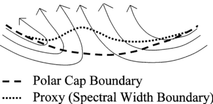
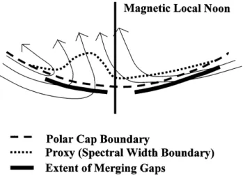
Fig. 1. A schematic representation of the relationship between the
spectral width boundary and the actual polar cap boundary in the ionospheric cusp region. The spectral width boundary is offset from the polar cap boundary in regions where the convection flow has a poleward component.
magnitude, and correlates well with the interplanetary elec-tric field input from the solar wind (Reiff et al., 1981; Doyle and Burke, 1983; Wygant et al., 1983). These studies have suggested a functional form for the cross-polar cap potential which has a linear dependence on the interplanetary electric field (Burke et al., 1999). The interplanetary electric field de-pends on IMF Byand Bz, and the solar wind velocity (Kan
and Lee, 1979). As a general rule, as IMF Bzbecomes more
negative, the polar cap potential increases.
The footprint of the open-closed field line boundary in the ionosphere is termed the polar cap boundary (PCB). The continual addition and removal of flux across this bound-ary, as a result of reconnection, is described in the expand-ing/contracting polar cap model (Siscoe and Huang, 1985; Cowley and Lockwood, 1992). The reconnection location (termed the X-line) on the magnetopause maps to a region in the dayside ionosphere termed the merging gap (Moses et al., 1987) which is a longitudinally-limited region of the PCB through which the ionospheric plasma flows into the polar cap. Identifying the PCB in the dayside ionosphere is crucial for studying the ionospheric signature of magnetic re-connection on the dayside magnetopause. At present, it is not always possible to directly observe the PCB in the dayside ionosphere, although there are features that provide proxies for the PCB position in the cusp (Rodger, 2000):
1. The equatorward boundary of the 630 nm cusp aurora (Milan et al., 1999);
2. The equatorward edge of the high spectral width region in HF radar data (termed the spectral width boundary, SWB) (Baker et al., 1995; Rodger et al., 1995), and 3. The equatorward edge of cusp ion precipitation in low
altitude satellite observations (Newell and Meng, 1991). These features represent observations of the equatorward boundary of the cusp particle precipitation and are hence dis-placed poleward from the true PCB due to time-of-flight ef-fects of the precipitating particles. The displacement depends on a number of factors:
1. The field-aligned distance from the reconnection X-line on the magnetopause to the ionosphere (which deter-mines the cusp ion travel time);
2. The reconnection electric field, which determines the speed of the flow through the merging gap;
3. The energy and pitch-angle distributions of the precipi-tating cusp ions which will also influence the ion travel time along the field line.
Recent work (Baker et al., 1997; Provan et al., 1998; Pin-nock et al., 1999; Chisham et al., 2001) has shown the impor-tance of using the SWB as a proxy for the PCB in the cusp. There is a growing understanding of the factors which result in the high spectral width values observed in the cusp region (Andr´e et al., 1999, 2000) and also those which influence the offset of the SWB from the actual PCB (Rodger and Pinnock, 1997; Lockwood, 1997; Rodger, 2000; Pinnock and Rodger, 2001). However, little attention has been paid to the effect of temporal and spatial variations in the factors influencing the offset. Understanding the factors that influence the offset is important if one wants to interpret small or mesoscale varia-tions in the SWB, i.e. to distinguish genuine variavaria-tions in the PCB from variations in the offset between the PCB and its proxy. Figure 1 displays a simplified schematic illustration of the relationship between the PCB and the SWB (or other proxy) in the cusp region (Rodger, 2000). The SWB is dis-placed from the PCB only within the ionospheric footprint of the merging gap where there is a poleward flow component across the PCB. Hence, the SWB variation can potentially be used as a diagnostic of the extent of the merging gap by identifying the longitudinal extent of the poleward displace-ment. In practice, this is rarely feasible, as the merging gap is typically much larger than the field of view of a single in-strument; the extent of the merging gap is thought to be typ-ically ∼ 3 h of magnetic local time (MLT) (Lockwood and Davis, 1996), or longer (Maynard et al., 1997; Nishitani et al., 1999). Pinnock and Rodger (2001) have observed this characteristic proxy variation in the combined SWB varia-tion of four SuperDARN HF radars covering ∼ 6 h of MLT.
In this paper, we study an extended interval of extremely steady solar wind and IMF conditions (Bz ∼By ∼ −10 nT)
during which the Halley HF radar in Antarctica observed a very localised 2◦ poleward distortion of the SWB in the morning sector close to magnetic local noon. The distortion was quasi-stationary in magnetic local time with a width of ∼1 h of MLT, and lasted for at least an hour (as the Halley radar field of view passed through it). By invoking the anti-parallel merging hypothesis (Crooker, 1979), we show that this distortion can be explained as a result of a localised in-crease in the displacement of the SWB from the PCB in the morning sector and does not represent structure in the PCB. This increased displacement results from the morning sector reconnection X-line on the magnetopause being located fur-ther from the Soufur-thern Hemisphere ionosphere than its af-ternoon sector counterpart, as predicted by the anti-parallel merging hypothesis during intervals when IMF Bz ∼ By.
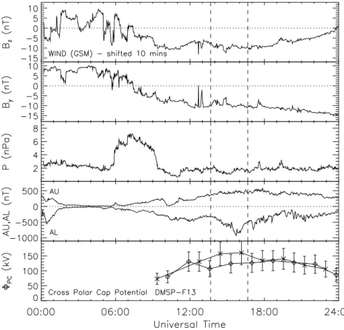
Fig. 2. Data presenting an overview of
solar wind and magnetospheric varia-tions on 20 August 1998. The panels show the interplanetary magnetic field
Bz and By components (in GSM
co-ordinates) and solar wind dynamic pres-sure from the WIND spacecraft, the AU and AL index variations, and the cross-polar cap potential estimate from DMSP-F13.
This results in a longer cusp ion travel time and hence, a greater displacement between the PCB and the SWB. By showing that the observed mesoscale variations in the SWB do not imply variations in the PCB on this occasion, we also demonstrate the importance of understanding the offset be-tween the PCB and its proxies.
2 Instrumentation
This study presents data from the SHARE (Southern Hemi-sphere Auroral Radar Experiment) HF radar pair located in Antarctica. The SHARE Halley and Sanae radars are part of the SuperDARN radar network. SuperDARN (The Super Dual Auroral Radar Network) is a network of co-herent scatter HF radars (Greenwald et al., 1995) which measure backscatter from magnetic field-aligned decametre-scale ionospheric irregularities. The radars transmit HF sig-nals which are refracted towards the horizontal as they en-ter ionospheric regions with higher electron concentrations. If these regions contain irregularities, the radar signals are backscattered when they are propagating perpendicular to the magnetic field (i.e. perpendicular to the irregularities). In the high-latitude ionosphere, these irregularities are of-ten present (Tsunoda, 1988); they move with the background plasma drift at F-region altitudes (Villain et al., 1985; Ruo-honiemi et al., 1987) and hence, provide information about large-scale convection and related processes in the radar field
of view. The radars transmit power at a fixed frequency in the range of 8–20 MHz and from the return signals, an estimate of the variation in backscatter power, line-of-sight Doppler velocity and Doppler spectral width in the radar field of view is derived (Baker et al., 1995 for details). Many of the Super-DARN radars have overlapping fields of view which means that line-of-sight Doppler velocities from these radars can be merged to produce two-dimensional velocity vectors.
The SHARE Halley radar is located at Halley, Antarctica (75.5◦S, –26.6◦E), and transmits in the direction of the
ge-omagnetic South Pole. The radar scan sweeps through 16 beam positions differing by 3.25◦ in azimuth. On the day studied in this paper (20 August 1998), the radar was operat-ing in a special mode which included three beams runnoperat-ing at a high time resolution. The integration time was 5 s for each beam and a full scan was made in 3 min, with each of the high time resolution beams repeating every 30 s. Each beam com-prised 75 range gates, with a pulse length of 300 µs (equiv-alent to 45 km) and a lag to the first range of 1200 µs (180 km). The SHARE Sanae radar (72.0◦S, –3.0◦E) shares a large, common field of view with the Halley radar and was operating in a similar mode at this time. Line-of-sight veloc-ities from the Sanae radar were merged with those from Hal-ley to produce field-perpendicular two-dimensional velocity vectors in the overlap region.
The SWB represents the boundary between the high spec-tral width values associated with regions of cusp ion
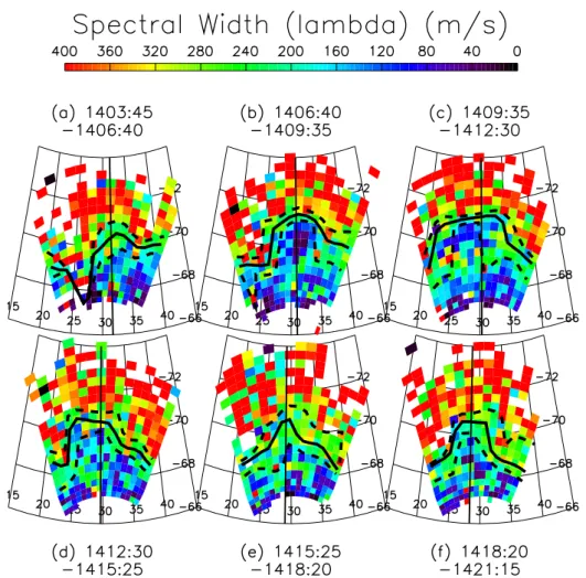
pre-Fig. 3. The spectral width variation in six consecutive scans from the Halley radar on 20 August 1998. The bold line enclosed by two dashed
lines represents the spectral width boundary and its uncertainty, respectively. The solid vertical line marks the longitude of 11:00 MLT.
cipitation and the low values observed in the regions equa-torward of the cusp (Baker et al., 1995). The wide and complex Doppler spectra which characterise the cusp result from electric field variations in the Pc1-2 frequency range (∼ 0.1–5 Hz) (Andr´e et al., 1999) which are thought to be related to the cusp precipitation. The spectral width is highly variable throughout the cusp; its distribution is approxi-mately Gaussian in nature, ranging from ∼ 100–600 m/s. Re-gions equatorward of the cusp are typically characterised by narrow Doppler spectra dominated by a single component. The spectral width in these regions is generally very low (< 100 m/s). Generally, the SWB is clearly defined at the equatorward edge of the ionospheric cusp. However, it must be stressed that caution is needed when interpreting high spectral widths in HF radar data, since there are a number of other sources of high spectral width unrelated to the cusp (Andr´e et al., 2000).
In this paper, we determine the SWB in the radar data using the method outlined by Chisham et al. (2001). In this method, the spectral width variation is first spatially smoothed and the SWB in each beam is taken as the point at which the smoothed spectral width variation first crosses 250 m/s. The method also requires that the average
spec-tral width over three range gates poleward of the suspected boundary position is > 250 m/s to eliminate the effect of oc-casional spectral width peaks at low ranges.
3 Event overview
On 20 August 1998, the WIND spacecraft was monitoring the solar wind approximately 65 RE upstream of the Earth,
displaced from the Earth-Sun line by ∼ 35 RE in the
neg-ative GSE y-direction. Figure 2 presents IMF Bz and By
and the solar wind dynamic pressure variations observed by WIND on this day, in the GSM coordinate system. The GEO-TAIL spacecraft, located approximately 30 RE upstream on
the Earth-Sun line, observed almost identical variations in these parameters with no large offset in the timing of signif-icant features in the early part of the day. However, a large data gap occurred in the GEOTAIL data between 12:00 and 19:30 UT and hence, the WIND data are shown. Since the variations seen by both spacecraft were so similar, we can be confident that despite its offset from the Earth-Sun line, the WIND observations describe well the solar wind that in-teracts with the Earth’s magnetosphere on this day. The two
spacecraft observations provide us with the means to make an accurate determination of the orientation of the solar wind phase front in the x − y plane on this day, allowing for an estimate to be made of the time delay from WIND to the ionospheric observations. We assume that any variation in the phase front in the z-direction will not significantly af-fect our time delay estimate. The WIND data in Fig. 2 have been shifted by 10 min to allow for the estimated time de-lay. Our ionospheric observations were predominantly con-fined to ∼ 13:40–16:40 UT (demarked by the vertical dashed lines in Fig. 2), an interval when the solar wind was very steady. Any uncertainty which exists in the time delay esti-mation is, therefore, of little importance to this study. The constant solar wind and IMF conditions allow us to spec-ulate that the magnetic reconnection scenario at the dayside magnetopause, and hence its ionospheric signature, remained quasi-steady during this interval.
During such an extended interval of large negative IMF Bz, the magnetosphere is usually very dynamic,
charac-terised by a number of substorm intervals. Figure 2 also shows the AU and AL index variations on 20 August 1998. After ∼ 06:00 UT, the AE index (AU-AL) grows steadily fol-lowing the southward turning of the IMF. However, there is little substorm activity; only minor substorms are evident, most notably at 15:20 UT and 17:00 UT. Much of the interval resembles an interval of “Steady Magnetospheric Convec-tion” (SMC) (Sergeev et al., 1996 for a recent review). SMC events are defined as periods of enhanced energy input from the solar wind into the magnetosphere over a time interval of several substorm time constants during which the large-scale stability of the magnetotail is sustained. For example, Yahnin et al. (1994) observed an interval of intense magneto-spheric convection which continued for more than 10 h under steady southward IMF conditions without any distinct sub-storm signatures. They observed that the dayside cusp was located at an unusually low-latitude (∼ 70◦) at this time. The existence of predominantly steady convection and minimal substorm activity during our event further suggests that the dayside convection scenario will be quasi-steady throughout this interval.
The final panel in Fig. 2 presents an estimate of the cross-polar cap potential variation from DMSP-F13. The DMSP spacecraft describe low altitude polar orbits of the Earth and measure plasma characteristics in the polar regions. DMSP-F13 is the operational DMSP spacecraft which was closest to a dawn-dusk orientation at this time and provided an es-timate of the cross-polar cap potential variation for our in-terval of study. Two data sets are presented; the diamonds represent northern hemisphere measurements, whereas the crosses represent southern hemisphere measurements. The values shown represent the observed potential variation along the spacecraft track, which is always less than the true total potential (Hairston et al., 1998). Typically, if the spacecraft orbit passes above 80◦magnetic latitude, then the measure-ment will represent 80–95% of the true potential. For the data shown, only three of the measurements were taken from orbital passes that did not exceed 80◦ and hence, the
ob-Fig. 4. (a) The statistical variation of the spectral width
bound-ary position with magnetic local time during the interval 13:50– 15:00 UT. Each symbol represents a single observation of the spec-tral width boundary taken from a single beam from a single 3-min scan. (b) The spectral width variation seen by Halley beam 8 dur-ing the interval 13:50–15:00 UT. (c) The spectral width variation seen by beam 3 during the interval 13:50–15:00 UT. The solid and dashed lines on all the panels represent the median and quartile vari-ations of the scatterplot observvari-ations.
served variation represents a true reflection of the cross-polar cap potential on this day. The potential measured is very large, typically ∼ 100–150 kV, which is not unusual during extended intervals of IMF Bz 0. There is very little
varia-tion in the potential during the steady solar wind interval; the potential is smaller at the start of the interval of data shown (immediately after the Bzsouthward turning) and at the end
of the interval of data (as Bzapproaches 0). During the
inter-val when we observed our strong radar backscatter (13:40– 16:40 UT), the observed potential was ∼ 100–160 kV. The difference between the observed potentials in the northern and southern hemispheres during this interval is attributed more to the differences in the satellite’s track across the po-lar cap regions in the two hemispheres, rather than to any intrinsic difference in the total potentials in each hemisphere.
4 Ionospheric observations
4.1 Spectral width boundary observations
On this day, the Halley and Sanae HF radars observed al-most 3 h (∼ 13:40 to 16:40 UT) of continuous backscatter
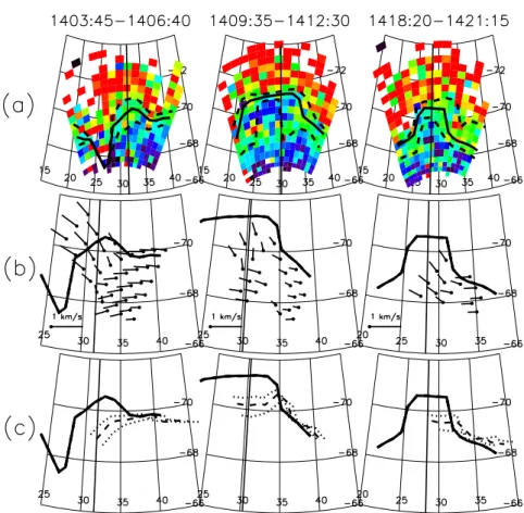
Fig. 5. Data from three Halley radar scans during the interval 13:50–15:00 UT (times shown). (a) The spectral width variation. The bold and
dashed lines represent the spectral width boundary (see text). (b) Comparison of merged velocity vectors and the spectral width boundary. (c) Comparison of the spectral width boundary (bold line) with the mapped estimates of the polar cap boundary (dashed and dotted lines, see text).
close to magnetic local noon (magnetic local noon at Halley was at ∼ 15:20 UT). During the interval 13:50–15:00 UT, the SWB variations in the 3-min full scans from the Halley and Sanae radars were characterised by a ∼ 2◦poleward dis-tortion of the boundary. This disdis-tortion was approximately stationary in MLT, being ∼ 1 h wide and centred at about 11:00 MLT. Figure 3 presents six consecutive scans from the Halley radar during the centre of this interval illustrating the spectral width variation across the field of view. The bold line surrounded by two dashed lines represents the location of the SWB and its uncertainty (as described by Chisham et al., 2001). This boundary provides a clear demarcation line between the high spectral width values in the cusp (predom-inantly red) and the lower spectral width values equatorward of the cusp (predominantly blue). The solid vertical line on each scan represents the longitude of 11:00 MLT. Each scan clearly shows the poleward distortion of the boundary centred on 11:00 MLT, although it does show the existence of small, temporal variations in its morphology. This
fea-ture was continually observed across the interval of 13:50– 15:00 UT, by the Halley radar, as its field of view passed over it. The afternoon edge of the feature was also continu-ally observed by the Sanae radar.
To illustrate the stability of this SWB feature, Fig. 4a presents a scatter plot of all the SWB positions estimated dur-ing this interval (for all 16 beams of the Halley radar in all the 3-min scans between 13:50 and 15:00 UT). The solid and dashed lines represent the median as well as the upper and lower quartile variations of the boundary position with mag-netic local time. It is clear from the figure that the poleward distortion of the boundary is a stationary feature during this interval. The scatter of the boundary positions results from the small, temporal variations in the boundary distortion, as shown in Fig. 3. To illustrate further the stability of this fea-ture, Figs. 4b and 4c show the spectral width variations for beams 8 (at 3-min resolution) and 3 (at 30-s resolution) of the Halley radar for the same time interval. The median and quartile variations from the scatter plot have been
overplot-ted on the spectral width data. The same variation is clearly visible in the measurements from these beams.
4.2 Convection flow observations
We now study the convection flow in the vicinity of the boundary distortion. Figure 5 presents the details of three of the individual 3-min scans from the Halley radar during this interval. Figure 5a presents the spectral width variations for these scans, as shown already in Fig. 3. Figure 5b compares enlarged sections of the measured boundaries (bold lines) with two-dimensional velocity vectors estimated by merg-ing the line-of-sight Doppler velocities from the Halley and Sanae radars. A clear pattern in the velocity field is appar-ent for all the scans during this interval where merged vec-tors could be estimated, including the three examples shown. Equatorward of the distortion of the SWB, the vectors are al-most exclusively westward. In the locality of the boundary distortion, the vectors possess a significant poleward com-ponent and the flow across the SWB appears predominantly confined to this region. This scenario is suggestive of the schematic illustration in Fig. 1 and could imply that the dis-tortion represents the extent of the merging gap on this day. This is considered in Sect. 4.4 of the paper. No merged vec-tors could be estimated outside the vicinity of this feature due to the lack of overlapping backscatter in the Halley and Sanae fields of view at earlier and later universal times. Hence, the full extent of the merging region in the dayside ionosphere could not be estimated from the radar data.
As discussed by Andr´e et al. (2000), spatial gradients in the large-scale convection pattern can enhance the spectral width values measured by the SuperDARN radars. Large gradients in the flow direction or magnitude within a sin-gle range cell can introduce several components into the spectrum measured in that range cell. Since the analysis method that is used to derive the spectral width is not well adapted to these spectra, the resulting spectral width will be enhanced. Andr´e et al. (2000) showed that a zonally-looking radar might measure a spectral width of ∼ 250 m/s in the re-gion of a convection reversal or large shear in the velocity field. However, for a poleward-looking radar (such as the Halley radar), the spectral width obtained from the same re-gion is reduced (to ∼ 150 m/s) due to the change in the geom-etry of the range cell with respect to the velocity shear. Andr´e et al. (2000) concluded that for meridionally pointing radars, the large spectral widths measured in the cusp could not be explained by gradients in the large-scale convection pattern. The effect of spatial variations in the convection flow on the spectral width can be seen in Fig. 5. All three scans show a clear change in the convection flow from westward to pole-ward in Fig. 5b, as discussed above. At these points there is a clear enhancement in the spectral width in Fig. 5a to ∼150–250 m/s (green shading). However, gradients in the convection flow cannot be used to explain the much larger spectral width values (>400 m/s) observed above the esti-mated SWB, which are a result of Pc1/2 wave activity as-sociated with cusp precipitation.
4.3 Estimating the polar cap boundary position
Using the merged velocity vector measurements, the SWB positions have been reverse mapped in order to determine an estimate of the PCB position (Pinnock and Rodger, 2000). To perform this mapping, an estimate of the magnetosheath-like ion travel time from the reconnection X-line to the ionosphere is required. Here, we assume the anti-parallel merging hypothesis and use the Tsyganenko 96 magneto-spheric field model (Tsyganenko, 1995; Tsyganenko and Stern, 1996) to determine the field-aligned distance from this ionospheric location to the estimated anti-parallel merging region on the magnetopause (Coleman et al., 2000, for full details of the determination of anti-parallel regions). For the prevailing IMF conditions, this distance was estimated to be ∼ 20.4–21.3 RE (see discussion section for further
de-tails). DMSP-F14 cusp particle observations at this time (not shown) suggested that the maximum cusp ion energies were in the range of 0.25–1.0 keV. These parameters predict an ion travel time from the reconnection X-line to the southern ionosphere of ∼ 300–600 s and hence, the offset of the SWB from the actual PCB will result from the motion of the newly-reconnected field lines with the convection flow during this time.
Figure 5c presents the results of mapping the observed SWBs using a velocity field determined from the measured vectors. Only the parts of the boundaries with local merged velocity vectors were mapped. In Fig. 5c, the two dotted lines represent the mapped boundaries (PCB estimations) for 300 s and 600 s ion travel times and the dashed line for 450 s. The second and third scans presented involve greater uncertainty in the mapped boundary position due to the necessary extrap-olation of the velocity field from the most poleward vectors to the observed SWB position. It is likely that the bound-ary offsets have been underestimated in these cases; the line-of-sight velocity variations show increasing poleward flows with latitude. It is also unlikely that the actual PCB posi-tion would be located poleward of the SWB posiposi-tion, as seen at the eastward edge of the second and third scans. This is most likely a result of uncertainties in the velocity field and measured SWB locations.
Although there exist uncertainties in the mapped bound-ary locations, a number of features of the estimated PCB po-sitions appear robust. First, the poleward distortion, a per-sistent characteristic of the observed SWB, has been largely reduced. In the vicinity of the distortion, the PCB estimate is a significant distance equatorward of the observed SWB (∼ 1◦), whereas outside this region, the boundary is rela-tively unchanged. This has largely removed the sharp pole-ward variation in the boundary at the edges of the distortion. Second, the PCB estimates appear to be located close to the change in the convection flow direction from westward to poleward, which is clearly apparent in the velocity vectors displayed in Fig. 5b.
Fig. 6. (a) The spectral width
varia-tion seen by Halley beam 3. The bold line represents an estimate of the spec-tral width boundary from the specspec-tral width observations. (b) The Doppler line-of-sight velocity variation seen by Halley beam 3. The vertical dashed line represents the transition between the two flow regimes seen by beam 3. The horizontal dashed lines denote the latitudes of the A80 and A81 magne-tometers. (c) The spectral width vari-ation seen by Halley beam 8. The bold line represents an estimate of the spec-tral width boundary from the specspec-tral width observations. (d) The Doppler line-of-sight velocity variation seen by Halley beam 8. (e) H -component mag-netometer data from the A80 and A81 (bold line) AGO magnetometers in the Antarctic. The vertical dotted lines de-lineate estimates of the boundaries be-tween the throat and return flow as esti-mated from the magnetometer data.
4.4 The morning sector reconnection potential
We suggested earlier that poleward excursions of the SWB, such as observed here, can be used as a diagnostic of the ex-tent of the merging gap (Rodger, 2000; Pinnock and Rodger, 2001). However, our velocity vector observations extend for less than 2 h of MLT and we are unable to determine the two-dimensional velocity field for large regions of the dayside ionosphere. However, we can use our velocity vector mea-surements and our estimated PCB positions to determine the reconnection potential in our field of view (using the method employed by Pinnock et al., 1999). For all the scans during this interval for which reconnection electric field estimates could be made, the reconnection potential estimate across the field of view (∼ 1.0–1.5 h of MLT) was never greater than 20 kV. Indeed, it was often less than 10 kV. The cross-polar cap potential measurements from DMSP-F13 at this time suggest a cross-polar cap potential of ∼ 100–150 kV (see Fig. 2). This suggests that the extent of the whole merg-ing region in the dayside ionosphere is much larger than the SWB distortion observed here. Consequently, the nature of
the observed morning sector merging region suggests the ex-istence of mesoscale variations in the overall dayside merg-ing scenario.
4.5 The extent of the dayside merging region
To understand the scenario on this day, we need to obtain a large-scale picture of the dayside convection flow. So far, we have studied in detail just over an hour of data from the SHARE radar pair. Figure 6 presents the full three hours of data for this interval from Halley beam 3 (at high time reso-lution) and beam 8 (at scan resoreso-lution) in geomagnetic lati-tude and magnetic local time coordinates and compares this with data from the Antarctic magnetometers. Halley beam 8 points poleward, along the magnetic meridian, and Halley beam 3 is directed at an angle of ∼ 16◦ to the west of the magnetic meridian.
Figure 6a presents the spectral width variation from beam 3 for this interval; the bold line represents the estimated lo-cation of the SWB using the same method as discussed in Sect. 2. The poleward distortion of the boundary is very
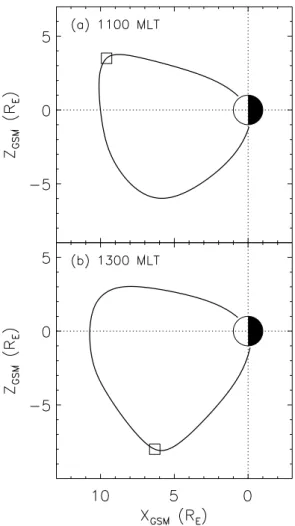
Fig. 7. Model representation of the last closed field line during
this interval, in GSM x-z coordinates at (a) 11:00 MLT, and (b) 13:00 MLT. The square symbols represent the locations of the es-timated anti-parallel reconnection X-lines.
clear, centred on 11:00 MLT. At later magnetic local times, the boundary is located close to –67◦latitude, although there appear to be occasional poleward excursions in the boundary. The largest of these excursions (at ∼ 15:00 MLT) appears to occur simultaneously on all beams (not shown), suggesting that they may represent temporal, and not spatial variations in the boundary position. Figure 6b displays line-of-sight velocity data from Halley beam 3; positive (negative) veloc-ities represent the line-of-sight flow toward (away from) the radar. Two flow regimes are apparent in the line-of-sight ve-locity data: strong flows above –71◦latitude in the morning
sector and strong flows above –67◦latitude in the afternoon sector. These flow regimes switch at ∼ 11:40 MLT (marked by the vertical dashed line in Fig. 6). There is a clear distinc-tion between the flows and the boundary posidistinc-tion observed in the local morning and those observed in the local afternoon. Figure 6c presents the spectral width variation from beam 8 for this interval. The observed SWB is very similar to that seen by beam 3 in Fig. 6a, albeit at a lower resolution. Fig-ure 6d displays the line-of-sight velocity data from beam 8.
It is immediately obvious that there is not the large distinc-tion between the flow regimes on either side of noon, as seen by beam 3; indeed, the line-of-sight velocities observed by beam 8 suggest that the poleward component of the convec-tion flow is approximately constant on either side of noon. The large afternoon sector flows observed by beam 3 are, therefore, a result of a large increase in the zonal (westward) component of the flow in the afternoon sector.
In order to determine how these flows relate to the larger-scale convection pattern, we have studied data from the A80 (–66.89◦, 27.99◦AACGM coordinates) and A81 (–69.17◦, 35.81◦AACGM coordinates) AGO magnetometers, located within the Halley radar field of view in the Antarctic. The magnetometer data can provide a crude qualitative estimate of the equivalent convection flow in the dayside ionosphere. The equivalent convection flow is estimated by: First, re-moving a close, quiet day variation (17 August 1998) from the magnetometer data; second, rotating the residual hori-zontal magnetic field vector by 90◦ anti-clockwise.
How-ever, the H -component observed by the magnetometers gen-erally provides a good estimate of the east-west component of the equivalent convection, whereas the D component can be severely affected by large field-aligned currents in the vicinity of the observations (Kamide et al., 1976). Hence, in Fig. 6e, we present the H -component variations (with the quiet day variation removed) from A80 and A81, which pro-vide a qualitative estimate of the zonal (east-west) compo-nent of the convection flow. Negative values represent east-ward flow (as in the dawnside return flow), whereas posi-tive values represent westward flow (as in the duskside re-turn flow). The band around zero represents a region of low zonal flow which corresponds to the throat flow region in the ionospheric convection pattern and provides an estimate of the extent of the merging region. The dotted vertical lines in Fig. 6 represent estimates of the location of the transitions between the return and throat flow regions. The A81 observa-tions do not clearly show a westward flow that represents the duskside return flow. However, it is likely that for much of the interval under study, A81 is located within the polar cap. Although they only provide a crude estimate of the changes in convection, the magnetometer observations suggest that the merging gap (the throat flow region) covers at least ∼ 3 h of magnetic local time on this day and extends well into the afternoon sector, outside the poleward distortion observed in the morning sector. These afternoon sector flows should cor-respond to a significant fraction of the observed cross-polar cap potential.
5 Discussion
The significant question raised by the observations presented in this paper is why is the SWB in the morning sector (as seen in our localised poleward distortion) located ∼ 2◦ pole-ward of that in the early afternoon sector? This does not represent a temporal change in the PCB position since the distortion is seen as a clearly distinct feature in the
spa-Fig. 8. A schematic representation of the relationship between the
spectral width boundary, the polar cap boundary, and the convection flow for the interval under study.
tial maps of spectral width (e.g. in Fig. 3). It is also not likely to represent a spatial variation in the actual PCB po-sition as the feature lasts for an extended interval (at least 1 h) and any large displacement of the PCB from a stable equilibrium position would be expected to be rectified on a shorter time scale. We can explain the difference as a re-sult of a change in the offset between the SWB and the PCB on either side of magnetic local noon. This could be due either to changes in the flow across the merging gap or to changes in the ion travel time from the reconnection X-line. This becomes an increasingly likely scenario if one consid-ers the consequences of the anti-parallel merging hypothesis (Crooker, 1979). During intervals when IMF Byis
compara-ble to Bz, the anti-parallel merging hypothesis predicts two
distinct reconnection X-lines on the dayside magnetopause (Crooker, 1979; Luhmann et al., 1984; Coleman et al., 2001). For By ∼ Bz < 0, the reconnection X-lines are located at
high-latitudes on the Northern Hemisphere magnetopause in the morning sector and on the Southern Hemisphere magne-topause in the afternoon sector.
Figure 7 presents estimates of the morphology of the morning (∼ 11:00 MLT) and afternoon (∼ 13:00 MLT) sec-tors’ last closed field lines for the conditions observed dur-ing this event, usdur-ing the Tsyganenko 96 magnetospheric field model. The squares in Fig. 7 represent the locations on these field lines where the geomagnetic field is antiparallel to a perfectly-draped magnetosheath magnetic field for these conditions (Coleman et al., 2000, for further details of this model). It is immediately obvious from Fig. 7 that the morn-ing sector reconnection X-line is located significantly further from the Southern Hemisphere ionosphere (∼ 21 RE
field-aligned distance) than the afternoon sector reconnection X-line (∼ 10 RE). This implies a longer ion travel time from
the reconnection X-line to the ionosphere in the morning sec-tor than in the afternoon secsec-tor. If we consider 500 eV pro-tons (the energy at which the cusp ion flux is a maximum, as observed by DMSP-F14), then the difference between the
morning and afternoon sector ion travel times is ∼ 230 s, i.e. significantly longer in the morning sector.
Figure 6d illustrates that the poleward component of the convection flow is similar in both the morning and after-noon sectors. Therefore, the proposed difference in ion travel times would cause the morning sector precipitation to be con-vected further poleward, explaining the much greater off-set between the SWB and the PCB in the morning sector. Assuming a poleward flow component of ∼ 400–500 m/s in both the morning and afternoon sectors (Fig. 6d) results in a predicted difference between the morning and afternoon sec-tor SWB offsets of ∼ 92–114 km, i.e. ∼ 1◦ latitude. This agrees fairly well with the poleward extent of the distortion observed in the spatial maps of spectral width in Fig. 3. How-ever, Figs. 4 and 6 present variations in the spectral width de-termined from temporal changes observed by single beams. The UT interval in which the data was collected is likely to have involved a period of polar cap expansion, as expected during an interval of extended southward IMF. Figure 4 illus-trates that the SWB dawnward of the edge of the distortion at 10:30 MLT (and dawnward of the merging region, and hence, where we would expect no poleward offset), is located at ∼– 69◦. This is at a higher latitude than the SWB observed in the afternoon sector, which may imply an equatorward motion of the PCB over the interval of study.
Another point to note is that the morning sector throat flow appears quasi-steady, whereas the high-resolution data show that the afternoon throat flow is extremely bursty with large line-of-sight velocity flow bursts in evidence. These flow bursts may imply pulsed reconnection and, as a result, transient poleward and equatorward motion of the polar cap boundary (consistent with models such as that of Cowley and Lockwood, 1992). The transient poleward motions of the SWB, evident in the afternoon sector in Fig. 6a, may be a re-sult of this. However, the possibility still exists that much of the SWB motion is a result of transient variations in the off-set between the SWB and the PCB and hence, the observed SWB motion may not completely reflect the motion of the PCB.
In Fig. 8, we attempt to summarise the observed scenario in a schematic diagram along the lines of Fig. 1. In the morn-ing sector, the convection flow poleward of the PCB is pre-dominantly poleward (as shown in Figs. 5 and 6). The large ion travel time from the reconnection location on the north-ern high-latitude magnetopause to the southnorth-ern ionosphere results in a large offset of the SWB from the PCB, leading to the observed poleward distortion. This distortion images the extent of the morning sector merging region. In the af-ternoon sector, the convection flow immediately poleward of the PCB is predominantly westward (as shown in Figs. 5 and 6), although the poleward component of the flow is similar to that observed in the morning sector (Fig. 6d). The smaller poleward offset of the SWB from the PCB in the afternoon sector is explained as a result of the shorter ion travel time from the reconnection location on the high-latitude Southern Hemisphere magnetopause to the southern ionosphere.
ionospheric signature of the cusp in the dayside ionosphere during an interval of quasi-steady solar wind conditions, we have been able to study the variations in the factors which determine the offset between the PCB and one of its proxies: the SWB. The lack of variability in the solar wind allowed us to observe a large region of the dayside ionosphere at a time when there was unlikely to be a significant variation in the reconnection scenario on the dayside magnetopause. If one assumes the anti-parallel merging hypothesis, then the difference in the SWB position observed on either side of magnetic local noon arises primarily from the difference be-tween the ion travel time from the morning and afternoon reconnection X-lines on the magnetopause to the Southern Hemisphere ionosphere. These results, therefore, provide ev-idence to support the anti-parallel merging hypothesis.
This study also highlights that mesoscale or small-scale variations in the SWB do not always represent variations in the PCB. Hence, it is important when using proxies for the PCB to understand the possible variations in the offset from the actual boundary. These variations can result from spatial or temporal changes in the convection flow across the merg-ing gap (i.e. in the reconnection rate), or from variations in the reconnection scenario on the magnetopause, which lead to changes in the ion travel time from the reconnection X-line to the ionosphere. These caveats apply to other proxies for the PCB which are related to cusp particle precipitation, such as the 630 nm cusp auroral emission. Indeed, it is pos-sible that some of the spatiotemporal structure of the cusp aurora is a result of mesoscale variations of this type.
Acknowledgements. The Halley and Sanae radars were developed
under funding from the NERC (UK), NSF (US), and DEAT (South Africa). Operations are supported by the NERC (UK) and DEAT (South Africa). DMSP data and analysis were provided under NSF grant ATM-9713436 and NASA grant NAG5-9297. The WIND data are part of the CDAWeb database. We are grateful to Dr. R. Lepping, principal investigator on the WIND MFI instru-ment. We would like to thank the Halley SHARE radar engineers, Kevin O’Rourke and David Glynn.
Topical Editor M. Lester thanks K. McWilliams and two other referees for their help in evaluating this paper.
References
Andr´e, R., Pinnock, M., and Rodger, A. S.: On the SuperDARN autocorrelation function observed in the ionospheric cusp, Geo-phys. Res. Lett., 26, 3353–3356, 1999.
Andr´e, R., Pinnock, M., Villain, J.-P., and Hanuise, C.: On the factors conditioning the Doppler spectral width determined from SuperDARN HF radars, Int. J. Geomagn. Aeron., 2, 77–86, 2000. Baker, K. B., Dudeney, J. R., Greenwald, R. A., Pinnock, M., Newell, P. T., Rodger, A. S., Mattin, N., and Meng, C.-I.: HF radar signatures of the cusp and low-latitude boundary layer, J. Geophys. Res., 100, 7671–7695, 1995.
Baker, K. B., Rodger, A. S., and Lu, G.: HF-radar observations of the rate of magnetic merging: a GEM boundary layer campaign study, J. Geophys. Res., 102, 9603–9617, 1997.
Burke, W. J., Weimer, D. R., and Maynard, N. C.: Geoeffective in-terplanetary scale sizes derived from regression analysis of polar cap potentials, J. Geophys. Res., 104, 9989–9994, 1999. Chisham, G., Pinnock, M., and Rodger, A. S.: The response of
the HF radar spectral width boundary to a switch in the IMF By
direction: Ionospheric consequences of transient dayside recon-nection? J. Geophys. Res., 106, 191–202, 2001.
Coleman, I. J., Pinnock, M., and Rodger, A. S.: The ionospheric footprint of antiparallel merging regions on the dayside magne-topause, Ann. Geophysicae, 18, 511–516, 2000.
Coleman, I. J., Chisham, G., Pinnock, M., and M. P. Freeman: An ionospheric convection signature of antiparallel reconnection, J. Geophys. Res., in press, 2001.
Cowley, S. W. H. and M. Lockwood: Excitation and decay of so-lar wind driven flows in the magnetosphere-ionosphere system, Ann. Geophysicae, 10, 103–115, 1992.
Crooker, N. U.: Dayside merging and cusp geometry, J. Geophys. Res., 84, 951–959, 1979.
Doyle, M. A., and Burke, W. J.: S3-2 measurements of the polar cap potential, J. Geophys. Res., 88, 9125–9133, 1983.
Greenwald, R. A., Baker, K. B., Dudeney, J. R., Pinnock, M., Jones, T. B., Thomas, E. C., Villain, J.-P., Cerisier, J.-C., Senior, C., Hanuise, C., Hunsucker, R. D., Sofko, G., Koehler, J., Nielsen, E., Pellinen, R., Walker,A. D. M., Sato, N., and Yamagishi, H.: DARN/SuperDARN: A global view of the dynamics of high-latitude convection, Space Sci. Rev., 71, 761–796, 1995. Hairston, M. R., Heelis, R. A., and Rich, F. J.: Analysis of the
iono-spheric cross polar cap potential drop using DMSP data during the National Space Weather Program study period, J. Geophys. Res., 103, 26 337–26 347, 1998.
Heelis, R. A.: The effects of interplanetary magnetic field orienta-tion on dayside high-latitude ionospheric convecorienta-tion, J. Geophys. Res., 89, 2873–2880, 1984.
Kamide, Y., Akasofu, S.-I., and Brekke,A.: Ionospheric currents obtained from the Chatanika radar and ground magnetic pertur-bations at the auroral latitude, Planet. Space Sci., 24, 193–201, 1976.
Kan, J. R. and Lee, L. C.: Energy coupling function and solar wind-magnetosphere dynamo, Geophys. Res. Lett., 6, 577–580, 1979. Lockwood, M. and Davis, C. J.: On the longitudinal extent of mag-netopause reconnection pulses, Ann. Geophysicae, 14, 865–878, 1996.
Lockwood, M.: Relationship of dayside auroral precipitations to the open-closed separatrix and the pattern of convective flow, J. Geophys. Res., 102, 17 475–17 487, 1997.
Luhmann, J. G., Walker, R. J., Russell, C. T., Crooker, N. U., Spre-iter, J. R., and Stahara,S. S.: Patterns of potential magnetic field merging sites on the dayside magnetopause, J. Geophys. Res., 89, 1739–1742, 1984.
Maynard, N. C., Weber, E. J., Weimer, D. R., Moen, J., Onsager, T., Heelis, R. A., and Egeland, A.: How wide in magnetic local time is the cusp? An event study, J. Geophys. Res., 102, 4765–4776, 1997.
Milan, S. E., Lester, M., Cowley, S. W. H., Moen, J., Sandholt, P. E., and Owen, C. J.: Meridian-scanning photometer, coherent HF radar, and magnetometer observations of the cusp: a case study, Ann. Geophysicae, 17, 159–172, 1999.
Moses, J. J., Siscoe, G. L., Crooker, N. U., and Gorney, D. J.: IMF
Byand day-night conductivity effects in the expanding polar cap
convection model, J. Geophys. Res., 92, 1193–1198, 1987. Newell, P. T. and Meng, C.-I.: Ion acceleration at the equatorward
J. Geophys. Res., 18, 1829–1832, 1991.
Nishitani, N., Ogawa, T., Pinnock, M., Freeman, M. P., Dudeney, J. R., Villain, J.-P., Baker,K. B., Sato, N., Yamagishi, H., and Matsumoto, H.: J. Geophys. Res., 104, 22 469–22 486, 1999. Pinnock, M., Rodger, A. S., Baker, K. B., Lu, G., and Hairston,
M.: Conjugate observations of the day-side reconnection electric field: A GEM boundary layer campaign, Ann. Geophysicae, 17, 443–454, 1999.
Pinnock, M. and Rodger, A. S.: On determining the noon polar cap boundary from SuperDARN HF radar backscatter character-istics, Ann. Geophysicae, 18, 1523–1530, 2001.
Provan, G., Yeoman, T. K., and Milan, S. E.: CUTLASS Finland radar observations of the ionospheric signatures of flux transfer events and the resulting plasma flows, Ann. Geophysicae, 16, 1411–1422, 1998.
Reiff, P. H., Spiro, R. W., and Hill, T. W.: Dependence of polar cap potential drop on interplanetary parameters, J. Geophys. Res., 86, 7639–7648, 1981.
Reiff, P. H. and Burch, J. L.: IMF By-dependent plasma flow and
Birkeland currents in the dayside magnetosphere 2. A global model for northward and southward IMF, J. Geophys. Res., 90, 1595–1609, 1985.
Rodger, A. S., Mende, S. B., Rosenberg, T. J., and Baker, K. B.: Si-multaneous optical and HF radar observations of the ionospheric cusp, Geophys. Res. Lett., 22, 2045–2048, 1995.
Rodger, A. S.: Ground-based ionospheric imaging of magneto-spheric boundaries, Adv. Space Res., 25, 7/8, 1461–1470, 2000. Rodger, A. S. and Pinnock, M.: The ionospheric response to flux transfer events: The first few minutes, Ann. Geophysicae, 15, 685–691, 1997.
Ruohoniemi, J. M., Greenwald, R. A., Baker, K. B., and Villain, J.-P.: Drift motions of small-scale irregularities in the high-latitude F region: An experimental comparison with plasma drift mo-tions, J. Geophys. Res., 92, 4553–4564, 1987.
Ruohoniemi, J. M. and Greenwald, R. A.: Statistical patterns of high-latitude convection obtained from Goose Bay HF radar ob-servations, J. Geophys. Res., 101, 21 743–21 763, 1996. Sergeev, V. A., Pellinen, R. J., and Pulkkinen, T. I.: Steady
magne-tospheric convection: A review of recent results, Space Sci. Rev., 75, 551–604, 1996.
Siscoe, G. L., and Huang, T. S.: Polar cap inflation and deflation, J. Geophys. Res., 90, 543–547, 1985.
Smith, M. F. and Lockwood, M.: Earth’s magnetospheric cusps, Rev. Geophys., 34, 233–260, 1996.
Tsunoda, R. T.: High-latitude F-region irregularities: A review and synthesis, Rev. Geophys., 26, 719–760, 1988.
Tsyganenko, N. A.: Modelling the Earth’s magnetospheric mag-netic field confined within a realistic magnetopause, J. Geophys. Res., 100, 5599–5612, 1995.
Tsyganenko, N. A. and Stern, D. P.: Modelling the global magnetic field of large-scale Birkeland current systems, J. Geophys. Res., 101, 27 187–27 198, 1996.
Villain, J.-P., Caudal, G., and Hanuise, C.: A SAFARI-EISCAT comparison between the velocity of F-region small-scale irregu-larities and the ion drift, J. Geophys. Res., 90, 8433–8443, 1985. Weimer, D. R.: An improved model of ionospheric electric po-tentials including substorm perturbations and application to the Geospace Environment Modeling November 24, 1996, event, J. Geophys. Res., 106, 407–416, 2001.
Wygant, J. R., Torbert, R. B., and Mozer, F. S.: Comparison of S3-2 potential drops with the interplanetary magnetic field and mod-els for magnetopause reconnection, J. Geophys. Res., 88, 5727– 5735, 1983.
Yahnin, A., Malkov, M. V., Sergeev, V. A., Pellinen, R. J., Aulamo, O., Vennerstr¨om, S., Friis-Christensen, E., Lassen, K., Danielsen, C., Craven, J. D., Deehr, C., and Frank, L. A.: Fea-tures of steady magnetospheric convection, J. Geophys. Res., 99, 4039–4051, 1994.