The use of iron charge state changes as a tracer for solar wind entry and energization within the magnetosphere

(1)

HAL Id: hal-00317186

https://hal.archives-ouvertes.fr/hal-00317186

Submitted on 1 Jan 2003

HAL is a multi-disciplinary open access

archive for the deposit and dissemination of

sci-entific research documents, whether they are

pub-lished or not. The documents may come from

teaching and research institutions in France or

abroad, or from public or private research centers.

L’archive ouverte pluridisciplinaire HAL, est

destinée au dépôt et à la diffusion de documents

scientifiques de niveau recherche, publiés ou non,

émanant des établissements d’enseignement et de

recherche français ou étrangers, des laboratoires

publics ou privés.

wind entry and energization within the magnetosphere

T. A. Fritz, T. H. Zurbuchen, G. Gloeckler, S. Hefti, Jie Chen

To cite this version:

T. A. Fritz, T. H. Zurbuchen, G. Gloeckler, S. Hefti, Jie Chen. The use of iron charge state changes

as a tracer for solar wind entry and energization within the magnetosphere. Annales Geophysicae,

European Geosciences Union, 2003, 21 (11), pp.2155-2164. �hal-00317186�

(2)

Annales Geophysicae (2003) 21: 2155–2164 c European Geosciences Union 2003

Annales

Geophysicae

The use of iron charge state changes as a tracer for solar wind entry

and energization within the magnetosphere

T. A. Fritz1, T. H. Zurbuchen2, G. Gloeckler2,3, S. Hefti2, and J. Chen1

1_{Boston University, Center for Space Physics, 725 Commonwealth Ave., Boston, MA 02215, USA} 2_{University of Michigan, Dept AO & SS, Ann Arbor, MI, 48109, USA}

3_{University of Maryland, Dept Physics, College Park, MD 20742-2425, USA}

Received: 17 September 2002 – Revised: 15 April 2003 – Accepted: 17 April 2003

Abstract. The variation of the charge state of iron [Fe] ions

is used to trace volume elements of plasma in the solar wind into the magnetosphere and to determine the time scales as-sociated with the entry into and the action of the magneto-spheric energization process working on these plasmas. On 2–3 May 1998 the Advanced Composition Explorer (ACE) spacecraft located at the L1 libration point observed a series of changes to the average charge state of the element Fe in the solar wind plasma reflecting variation in the coronal tem-perature of their original source. Over the period of these two days the average Fe charge state was observed to vary from +15 to +6 both at the Polar satellite in the high lati-tude dayside magnetosphere and at ACE. During a period of southward IMF the observations at Polar inside the magne-tosphere of the same Fe charge state were simultaneous with those at ACE delayed by the measured convection speed of the solar wind to the subsolar magnetopause. Comparing the phase space density as a function of energy at both ACE and Polar has indicated that significant energization of the plasma occurred on very rapid time scales. Energization at constant phase space density by a factor of 5 to 10 was observed over a range of energy from a few keV to about 1 MeV. For a de-tector with a fixed energy threshold in the range from 10 keV to a few hundred keV this observed energization will appear as a factor of ∼ 103increase in its counting rate. Polar obser-vations of very energetic O+ions at the same time indicate that this energization process must be occurring in the high latitude cusp region inside the magnetosphere and that it is capable of energizing ionospheric ions at the same time.

Key words. Magnetospheric physics (magnetopause, cusp,

and boundary layers; magnetospheric configuration and dy-namics; solar wind-magnetosphere interactions)

Correspondence to: T. A. Fritz (fritz@bu.edu)

1 Introduction

The most striking and significant finding of the Polar satel-lite is that energetic particles are observed to be consistently and continuously present in the high latitude, high altitude dayside magnetosphere where they cannot be stably trapped. The source of these particles remains a topic of debate and scientific discussion. There are three sources under active consideration as the supplier of these particles. Source 1 has the particles produced upstream of the magnetosphere at the location of the bowshock when a “quasi-parallel” condition exists between the bowshock normal and the interplanetary magnetic field. Once energized in such a configuration the particles then move along their trajectories guided by the magnetic field and arrive in the dayside cusp.

Source 2 has the particles being accelerated in situ in the cusp/cleft region by an unknown mechanism in association with deep diamagnetic cavities that have been observed to be coexistent with enhanced fluxes of the energetic particles and the penetration of shocked solar wind inside the magne-topause. Once the particles are energized they are subject to gradient and curvature effects in the geomagnetic field and will drift away from the cusp location.

Source 3 has the particles being energized by processes in the geomagnetic tail associated with substorms. The parti-cles then drift to the dayside where over a narrow range of nightside radial distances they will move into the cusp when drifting to the dayside. This happens because the minimum along a magnetic field line near the dayside magnetopause is no longer at the equator but bifurcates and moves into each of the high altitude cusps. The azimuthal drift motion of these particles will follow the minimum of the magnetic field into either cusp.

Two of these sources (1 and 3) are consistent with the present ideas within the accepted paradigm for the way in which the magnetosphere functions. Source 2 will require a major change in these ideas. All three of these mechanisms may be active to some degree and may generate some ener-getic particles that show up in the cusp. Rather than argue

(3)

against the role of sources 1 and 3, which, due to geometry alone and the time variable nature of their acceleration pro-cess, will have difficulty in producing energetic particles on a continuous basis, this paper will concentrate on source 2, and will present evidence that shocked solar wind ions enter the high altitude, high latitude cusp/cleft from the magne-tosheath and are energized very rapidly to 100 s and 1000 s of keV. These shocked solar wind ions apparently produce individual diamagnetic cavities in which the magnetic field is observed to decrease from ∼100 nT to values approaching zero with a great deal of magnetic field turbulence associ-ated with the cavity (Chen et al., 1997, 1998; Fritz, et al., 1999). The power contained in the fluctuations is correlated to the intensity of the MeV ions observed (Chen and Fritz, 1998). The mechanism associated with this process seems to be continually active, but individual cavities are impulsive in nature with an event having an apparent lifetime of a few tens of minutes. These facts appear to be well-established by the charge-state, composition, and energy spectral mea-surements that have been made with Polar, in comparison to simultaneous Geotail measurements in the region upstream and downstream of the bowshock (Chen and Fritz, 1998; Fritz and Chen, 1999a, b).

The proposed cusp mechanism is capable of producing an energetic particle layer that straddles the magnetopause along the flanks of the magnetosphere and of filling the pseudo-trapping region on the dayside of the magnetosphere with energetic particles where they are often observed to ex-hibit striking energy dispersion signatures (Karra and Fritz, 1999; Fritz et al., 2000). Many authors have reported ob-servations of these energetic particles in the magnetosheath near the magnetopause (Meng and Anderson, 1970; Sarris et al., 1976; Baker and Stone, 1978; Williams et al., 1985). These particles can enter the magnetosphere as a result of gradients in the magnetic field and the resultant drifts they cause; ions entering along the dawn flank drifting to the west and electrons entering along the dusk flank drifting east will carry a current. They provide a rapid coupling of the vari-ations in the subsolar region to the substorm region of the tail magnetosphere. They will also be the source population for the radial diffusion process, which does a very good job of explaining the radial variation of radiation belt fluxes as a function of energy. This result has the potential to be a new paradigm for the way we view the source of particles and flow of information in the magnetosphere.

In this paper we will discuss a particularly fortuitous event on 2–3 May 1998 in the solar wind, which was monitored by the Advanced Composition Explorer (ACE) satellite up-stream of the Earth’s magnetosphere at the L1 libration point. This event permitted an element of solar wind plasma to be traced into the Earth’s magnetosphere, where it will be shown that the Polar satellite observed the same plasma over a series of high latitude passes through the dayside region. A com-parison of the phase space density of the same plasma ele-ments at the location of ACE and Polar calculated from these observations provide a definitive indication that the shocked solar wind is energized to 10 s, 100 s and even 1000 s of keV

in the high latitude subsolar magnetosphere region immedi-ately upon entry into the magnetospheric cusps.

2 Instrumentation

The ACE spacecraft was launched on 25 August 1997 and was injected into a halo orbit around the L1 libration point in December 1997. The Solar Wind Ion Composition Experi-ment (SWICS) (Gloeckler et al., 1998) determines uniquely the chemical and ionic-charge composition of the solar wind, the temperatures and mean speeds of all major solar-wind ions, from H through Fe, at all solar wind speeds above 300 km/s (protons) and 170 km/s (Fe+16), and resolves H and He isotopes of both solar and interstellar sources. SWICS measures the distribution functions of both the in-terstellar cloud and dust cloud pickup ions up to energies of 100 keV/e and makes a complete measurement of the Fe ion spectrum in 12 min. Another experiment on ACE is the Elec-tron, Proton, and Alpha Monitor (EPAM) particle instrument (Gold et al., 1998). EPAM is composed of five telescope apertures of three different types. Two Low Energy Foil Spectrometers (LEFS) measure the flux and direction of elec-trons above 30 keV, two Low Energy Magnetic Spectrome-ters (LEMS) measure the flux and direction of ions greater than 50 keV, and the Composition Aperture (CA) measures the elemental composition of the ions. The telescopes use the spin of the spacecraft to sweep the full sky. Solid-state detectors are used to measure the energy and composition of the incoming particles.

Polar was launched into a 1.8 by 9 RE orbit on 24 Febru-ary 1996 with an inclination of 86 degrees. On board Polar, the Magnetospheric Ion Composition Spectrometer (MICS), a part of the Charge and Mass Magnetospheric Ion Compo-sition Experiment (CAMMICE) is a 1-dimensional time-of-flight electrostatic analyzer with post acceleration measuring the ions with an energy/charge of 1 to 220 keV/e with very good angular resolution. The MICS, mounted perpendicular to the spin axis, is able to obtain a 2-dimensional distribu-tion at one energy per charge during each six-second spin riod. A complete energy spectrum is obtained in 32 spin pe-riods. The Imaging Proton Spectrometer (IPS), a part of the Comprehensive Energetic Particle and Pitch Angle Distribu-tion (CEPPAD) experiment (Blake et al., 1995) uses an ion-implanted solid-state detector that is discretely segmented into multiple pixels. The detector sits behind a collimation stack at the “focal plane” of a “pin-hole camera”, thereby imaging a slice of phase space. Three identical heads, each with three non-overlapping look directions (20◦×12◦) pro-vide collectively an instantaneous snapshot of a 180◦×12◦ wedge of phase space. As a consequence of spacecraft rota-tion, the IPS maps out a full 4pi steradian image each spin period (∼6 s). Flux measurements over a nominal energy range from 20 keV to a few MeV are obtained as a function of pitch-angle and energy each 1/32nd of a spin. The HYDRA experiment (Scudder et al., 1995) is a collection of electro-static analyzers designed for high resolution observations of

(4)

T. A. Fritz et al.: Solar wind entry and energization 2157

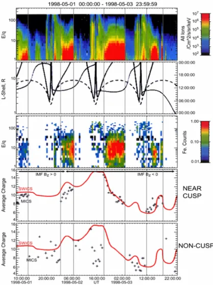
Fig. 1. Polar CAMMICE plasma data

for 1–3 May 1998. (a) Total ion in-tensity, (b) orbital parameters for the Polar satellite showing the radial dis-tance (broken line) and L-shell (heavy solid line) with the scale on the left axis and Magnetic Local Time, MLT (lighter solid line) with scale on the right side axis, (c) the intensity of the Fe ions, (d) the average charge state of the Fe ions measured by the ACE SWICS instru-ment (red line) and measured by Polar in the region of the cusp/cleft (+), (e) same as above except the Polar mea-surements are in regions other than the cusp/cleft. This figure has been modi-fied from Fig. 1 of Perry et al. (2000).

electron and ion velocity distributions between ∼2 keV/e and 35 keV/e in three dimensions with a routine time resolution of 0.5 s. Using other operational modes of the Hydra exper-iment it is possible to extend the lower limit of the measure-ment to 10 eV/e.

3 Observations and discussion

During the period of 2–3 May 1998, the SWICS instrument on the ACE satellite at the L1 libration point observed a vari-ation in the charge state of the solar wind Fe ions that ranged from an average value of +6 to +15 (Gloeckler et al., 1999). At the same time the Polar satellite observed a similar se-ries of changes in the charge state of Fe ions measured inside the magnetosphere in the vicinity of the dayside high alti-tude cusp. The comparison of measurements from the two satellites has been reported by Perry et al. (2000), and here, Fig. 1 is a slightly modified version of Fig. 1 from their paper. Perry et al. discussed the measurement techniques on the two satellites, the implication of the variation of Fe charge state in the solar wind, and provide a comparison of the average Fe charge states. In Fig. 1 the measurement at ACE are one-hour

averages and are represented by the red curve. The measure-ments at the position of Polar are given as the plotted “+”. The time scale for the ACE measurements was corrected for the propagation time from the L1 point to the subsolar mag-netopause based on the measured solar wind velocity. Note that over the two and a half day period presented in Fig. 1 the average charge state of Fe ions measured by ACE varied initially from a value of +10, rising to +15 and then tran-sitioning down to +6. This corresponded to changes in the coronal source temperature of 4×105to 2×106K.

Perry et al. (2000) have reported these measurements and their relationship to the timing of the arrival of a CME and some companion geomagnetic activity that followed. They concluded that during the period of southward interplanetary magnetic field indicated in Fig. 1 a very good correlation be-tween the measurements at ACE and at Polar was found, in-dicating that both spacecraft were sampling the same CME plasma population. The time scales of these observations were consistent with direct and rapid entry of solar wind plasma into the magnetosphere, concluding that this entry was via a subsolar magnetic field line merging site. In Fig. 1 there are four periods when Polar was on the dayside at high

(5)

Comparison of Phase Space Density measured at ACE and Polar on May 2, 1998 near 1900 UT

1.0E-05 1.0E-04 1.0E-03 1.0E-02 1.0E-01 1.0E+00 1.0E+01 1.0E+02 1.0E+03 1.0E+04 1.0E+05 1.0E+06 1.0E+07 1.0E+08 -1.0 0.0 1.0 2.0 3.0

Log of energy [keV/e]

f(v) [s^3km^-6] Hydra f(v) ACE SWICS f(v) MICS DCR f(v) MICS H+ f(v) IPS f(v) ACE-EPAM f(v)

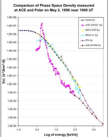
Fig. 2. The phase space density of the total ion population

deter-mined by the SWICS and EPAM instruments at ACE and by the HYDRA, MICS, and IPS instruments on Polar, as a function of en-ergy/charge. The two populations correspond to a plasma with an average Fe charge state of +15 recorded just before 19:00 UT on 2 May at ACE and just after 19:00 UT at Polar.

latitude and high altitudes, labeled as “near cusp”. The com-parison of the Fe charge state during these periods is given in the fourth panel, and a fifth panel is included showing the same comparison during the “non-cusp” periods. Perry et al. (2000) presented the details of the Polar cusp/cleft peri-ods in their Table 1. That table is reproduced here as Table 1 with an added column for the difference of the Start and End times. The feature to note in the table is the extended period of time in which Polar was located in the cusp/cleft or rather in a shocked solar wind plasma population that had recently and directly entered the magnetosphere. These observations are not consistent with the concept of a narrow funnel-shape cusp geometry. Fritz et al. (2003) have shown that contact by the Polar satellite with a very wide extended region of solar wind plasma entry is a common occurrence along the orbit of Polar, when the orbital plane is within a few hours of local noon.

From the response of the instruments on the ACE space-craft and on the Polar satellite it is possible to construct an energy spectrum from about 1 keV/e to beyond a few MeV for the dominant proton particle species. On Polar this range can be extended below 0.1 keV/e by the Hydra instrument. Selecting period #3 in Table 1 and Fig. 1 the average value

Table 1. Details of the Polar cusp/cleft periods

Period Date Start End Difference L1 L2 UT UT (hours) (degs) (degs) 1 1-May 10:30 13:00 2.5 80.3 85.9 2 2-May 2:30 7:00 4.5 73.3 82.0 3 2-May 20:00 3:00 7.0 75.8 85.4 4 3-May 13:30 16:00 2.5 76.4 83.3

of the iron charge state is observed to vary from +15 down to +8 over the duration of the seven-hour period where Polar continuously observed the shocked solar wind plasma. The tracking of the Fe charge states in the two data sets indi-cates that both are observing the same solar wind plasma. In other words, an element of solar wind plasma is “tagged” as it passes ACE and is then observed by Polar inside the magnetosphere with delays that are only associated with the solar wind propagation from ACE to the subsolar magne-topause. From the measured values of the particle fluxes,

j (particles/cm2 s sterradian keV) as a function of energy, the phase space density, f (s3/m6) = 5.45×10−31j/Energy (keV) can be calculated at the location of the two spacecraft. In the absence of sources and losses, Liouville’s theorem states that the density of particles in phase space, f , is con-stant along the particle trajectory.

Figure 2 compares the phase space densities as a function of energy/charge measured at the two spacecraft for the same “tagged” element of plasma. The two populations corre-spond to plasma with an average Fe charge state of +15 aver-aged for the 30-min period just before 19:00 UT on 2 May at ACE and averaged for the 30-min period following 19:00 UT at Polar. The comparison in Fig. 2 also indicates that the plasma has not only been thermalized, but it has been en-ergized significantly along its trajectory from ACE to Polar over a range of energy from a few keV to about one MeV. Note the agreement and consistency of the responses of the independently calibrated sensors on the two spacecraft. The particle energization at constant phase space density is be-tween a factor of five and ten. More significantly, however, is the fact that an instrument with a constant energy thresh-old would observe about a three order of magnitude increase in the particle flux it would measure as a result of this ener-gization. In the comparison of Fig. 2 the maximum in phase space density is the peak in the solar wind, and the solar wind fluxes are fully capable of being the source of the population measured at Polar.

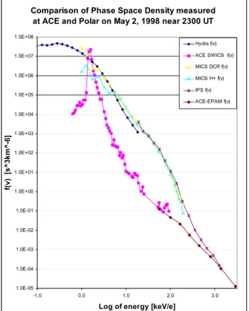
A comparison of the phase space densities at the two spacecraft using an element of plasma tagged with an av-erage Fe charge state of +10 is presented in Fig. 3. The ACE data are averaged over the 30-min period prior to 23:00 UT, and the Polar data are averaged over the 30-min period af-ter 23:00 UT. There has been little change in the solar wind phase space density measured at ACE, with the peak at about 3×107s3km−6. The phase space densities at the position of Polar show the same general characteristics but are different

(6)

1.0E-05 1.0E-04 1.0E-03 1.0E-02 1.0E-01 1.0E+00 1.0E+01 1.0E+02 1.0E+03 1.0E+04 1.0E+05 1.0E+06 1.0E+07 1.0E+08 -1.0 0.0 1.0 2.0 3.0

Fig. 3. Same format as Fig. 2 but now the two populations

corre-spond to a plasma with an average Fe charge state of +10 recorded just before 23:00 UT on 2 May at ACE and just after 23:00 UT at Polar.

in a fundamental way. The thermalization and significant en-ergization of the plasma is again evident but now the peak in the phase space density at ACE is less than that at Polar. The solar wind plasma is not fully capable of supplying all of the particles measured by Polar. There must be an addi-tional source of plasma at Polar. The most likely source of this additional plasma population is the Earth’s ionosphere, and the most likely such ion is O+ that can flow out of the ionosphere via the cleft ion fountain (Lockwood et al., 1985; Moore et al., 1985).

The CAMMICE MICS sensor has the capability to exam-ine the charge-state composition of the energized plasma to determine if there might be fluxes of ions of ionospheric ori-gin. In Fig. 4 the response of the MICS sensor to all major ion species is presented. The top panel displays oxygen ions with high charge-state oxygen, indicative of ions that originate in the solar wind. In the second panel the fluxes of oxygen ions with charge states associated with an ionospheric source are displayed. The threshold energy of ∼50 keV for the detec-tion of these O+, O++ions is much higher than that of O+6 shown in the first panel. The reason for this is that the MICS energy measurement is done by a solid-state detector with a contact dead layer that must be penetrated by the respective ion. In the case of O+6the post acceleration of 20 KV pro-vides 120 keV of addition energy to the ion permitting the

full range of these ion energies to be measured, if desired. In the case of O+_{they receive only an additional 20 keV of} en-ergy, which is not sufficient to penetrate the detector contact, resulting in an energy threshold of ∼50 keV. The third and fourth panels display the fluxes of helium ions, with the third panel being alpha particles and the fourth panel being singly charged helium. The fifth panel shows the total H or hydro-gen intensity. We see the seven-hour period from 19:00 h on 2 May to 03:00 h on 3 May easily identified with intense fluxes of high charge-state oxygen, alpha particles and hy-drogen. The magnetic field for this interval is displayed in the lower-right inset of Fig. 4. During this interval, Polar moves from a region of northward pointing magnetic field, through a very turbulent, depressed, and highly variable re-gion but variable around a constant level, until the satellite leaves the depressed field region where its encounters a field directed earthward. The Z component was negative through-out the highly turbulent region associated with this shocked solar wind plasma.

It is possible with the CAMMICE MICS to evaluate the phase space densities as a function of their parallel and per-pendicular velocities. For the interval covered by the data in Figs. 2 and 3 and in between, we display in Fig. 5 the phase space distribution at all energies in the top portion of the panel, and we zoom in on the distribution at lower ener-gies in the bottom panel. Note that the distribution at 19:15 h is basically an isotropic distribution with a small prefer-ence for 90-degree pitch angles as the distribution evolves in time. The preference for a trapped distribution contin-ues, but toward the end of the sequence, the distribution still takes on a broad, hemispherical distribution, with the peak at v-perpendicular but indicating that the direction away from the Earth was unable to maintain a trapping geometry. The lack or decrease of particle fluxes in the direction parallel to the magnetic field is consistent with the conclusions that the energized fluxes are coming from the direction of the Earth.

Returning to the observations in Fig. 3 in that an additional source of ions is required to supply the fluxes or phase space density seen at Polar during this interval, we see in Fig. 4 that ions most likely of ionospheric origin are present. These are He+and O+. It is possible to examine the ion composition Polar data in greater detail. In Fig. 6 we display the ion com-position data for the period of Fig. 2 using only those data that produce a valid time-of-flight (TOF) without a compan-ion valid energy response. This display will permit the MICS instrument to examine the lowest energy oxygen ions that it is capable of detecting. We show in the top panel those ion responses that are restricted to “zero energy”. When these responses are analyzed, looking now at the TOF versus E/q panel, we see that there are basically three main ion groups: H+, He++, and O+. There is also some He+ but the O+ clearly stands out as a line on top of the background, in-dicating a significant O+ population. Note also the energy of the O+ ions depicted by the E/q axis which indicates that these ions out of the ionosphere had energies from 1 to 100 keV. The energies indicate that these O+ions have un-dergone significant energization from their parent population

(7)

Fig. 4. The intensity of the ion species,

H+, He++, He+, O+, and high charge state O, as a function of particle en-ergy for the period of 2 and 3 May 1998. Note the three periods in which an extended signature of high charge-state 1–10 keV ions was seen along the trajectory of the Polar satellite. The or-bit projected onto the SM XZ-plane is also shown with an indication of where these extended signatures are seen. For the interval of Period 3 in Table 1 an inset showing the variation of the to-tal magnetic field is shown (courtesy of C. T. Russell), demonstrating the de-pressed magnetic field associated with the extended signature of high charge-state ions.

Fig. 5. The phase space distribution at all energies as a function of

the parallel and perpendicular particle velocities in the top portion of the panel and the same distribution at lower energies in the bot-tom panel determined using the double coincidence response [DCR] of the Polar MICS senor.

in the ionosphere. It seems likely that the energization pro-cess for the solar wind ions and these ionospheric ions is lo-cated at the same place. We believe the energization of both parent populations to energies equivalent to those responsible for the ring current occurs in the diamagnetic cavities associ-ated with the depressed field regions observed to be coexis-tent with the shocked solar wind plasma intrusion inside the

magnetosphere (Chen and Fritz, 2001). In Fig. 7 the detailed energy spectrum on each of the ion species measured by Po-lar is presented. The curve labeled Oois for oxygen ions with

charge states associated with a source in the ionosphere de-termined with the “zero energy” technique described above. As determined previously from Fig. 6 there are large fluxes of very energetic oxygen ions of ionospheric origin coexist-ing with the energized ions of solar wind origin durcoexist-ing the time period from 19:00–19:30 UT. The fluxes of Oo above

6 keV/e are equivalent to those of solar wind He++_{and are} the dominant oxygen ion during this period. The detailed en-ergy spectra for ions measured during the period from 23:00– 23:30 UT is displayed in Fig. 8. Again, there were apprecia-ble fluxes of oxygen ions of ionospheric origin present. They were nearly equivalent but were not the dominant oxygen ion species in this case for energies above 2 keV/q; at energies of 1 keV/q and below they probably dominate the helium and higher charge-state oxygen ions. This is most likely why the phase space density at Polar in the region below 1 keV/q ex-ceeds the phase space density of the solar wind source ions.

In Fig. 9 the phase space densities measured at the ACE spacecraft and at Polar at 02:00 UT on 3 May are compared. The ACE measurements were averaged for the 30-min period prior to 02:00 UT and the Polar measurements were already for the 30-min interval following 02:00 UT. Again, we ob-serve that the comparison of phase space densities indicates that thermalization and significant energization had occurred in the fluxes measured at Polar. Again, the phase space den-sity measured by the ACE spacecraft was unable to supply all of the particles needed to generate the phase space den-sities measured at Polar at this time. The average charge state of the Fe ions is +8 during this interval. When the de-tailed ion energy spectra are examined (Fig. 10) we again

(8)

Fig. 6. Display of the ion composi-tion direct event data for the period of Fig. 2 using only those data that pro-duce a valid time-of-flight (TOF) with-out a companion valid energy response.

Fig. 7. The energy spectrum of flux versus energy/charge of the

four major ion species determined for the interval from 19:00 UT to 19:30 UT on 2 May 1998.

see a significant presence of ions of ionospheric, as well as solar wind origin. The tendency noted above for the iono-spheric ions to become the dominant minor ion species below 1 keV/q is again consistent with the fact that the phase space density at Polar below 1 keV/q dominated those measured by ACE upstream in the solar wind.

As can be seen in the Fig. 1, around 03:00 UT, Polar left local times associated with the dayside and proceeded into

the nightside magnetosphere, leaving at the same time the re-gion of shocked solar wind plasma. The Polar satellite moved down through the radiation belts, over the southern polar re-gions, back out through the radiation belts, and again entered the high latitude dayside region in the vicinity of the magne-tospheric cusp. Slightly after 13:00 UT it again encountered an extended region of shocked solar wind plasma, noted as Period 4 in Table 1. When the Fe charge state was

(9)

deter-Comparison of Phase Space Density measured at ACE and Polar on May 3, 1998 near 0200 UT

1.0E-06 1.0E-05 1.0E-04 1.0E-03 1.0E-02 1.0E-01 1.0E+00 1.0E+01 1.0E+02 1.0E+03 1.0E+04 1.0E+05 1.0E+06 1.0E+07 1.0E+08 1.0E+09 -1.0 0.0 1.0 2.0 3.0

1.0E-06 1.0E-05 1.0E-04 1.0E-03 1.0E-02 1.0E-01 1.0E+00 1.0E+01 1.0E+02 1.0E+03 1.0E+04 1.0E+05 1.0E+06 1.0E+07 1.0E+08 1.0E+09 -2.0 -1.0 0.0 1.0 2.0 3.0

f(v) [s^3km^-6] Hydra f(v) ACE f(v) DCR f(v) H+ f(v) IPS f(v) ACE-EP

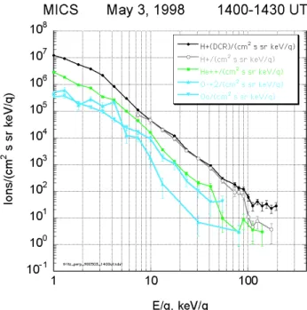
mined it again followed in time that measured upstream by the ACE spacecraft. A comparison was made for the same plasma element, this time with an average Fe charge state of six to seven at the two spacecraft near 14:00 UT. This com-parison of phase space densities measured at two spacecraft is presented in Fig. 11 with the same thermalization and sig-nificant energization occurring at Polar, but again the phase space densities measured by ACE were inadequate to pro-vide the necessary particles measured by the Polar space-craft. This region of shocked solar wind plasma with the ion composition dominated by ions H+_{, He}++_{and high} charge-state oxygen was apparent in the interval from 14:00 UT to beyond 18:00 UT in Fig. 4. From Fig. 1 we see that Po-lar stayed in the region of shocked soPo-lar wind plasma until the spacecraft moved from those local times associated with the dayside toward local times associated with the nightside magnetosphere. Figure 12 displays the detailed energy spec-tra at Polar for the major and minor ion species. Although He++ was the dominant minor ion species at all energies, there were significant fluxes of low charge-state ionospheric ions at all energies that displayed a similar spectral shape when compared to the species from the solar wind.

During the intervals analyzed in Figs. 2, 3, 9, and 11, we have observed a consistent pattern in which an element of plasma was followed from the solar wind at the L1 libration

(10)

point to the Polar spacecraft inside the magnetosphere. In each of these cases the interplanetary magnetic field (IMF) had a southward component. This geometry favors subsolar reconnection and easy entry of such plasma into the mag-netosphere. There was a period earlier on 2 May when the interplanetary magnetic field had a northward geometry that would not favor subsolar reconnection and easy plasma en-try. If Fig. 4 is examined, Polar was in a similar cusp-like environment from 02:00 UT until almost 07:00 UT, observ-ing a shocked solar wind plasma (Period 2 in Table 1), and we see in Fig. 1 that the close association in time of the Fe charge-state variation at ACE and at Polar is no longer appar-ent. There appears to be a similar slope to the variation of the charge state with time, but with a delay between those mea-surements made at Polar compared with those at the ACE spacecraft. It is instructive to examine the phase space den-sities at the two locations during this period. The interval around 06:00 UT was chosen for such a comparison. This is shown in Fig. 13 and again, we see that the plasma was ener-gized upon entry into the magnetosphere, but the entry was delayed by a significant time interval of a few hours. In Fig. 1 the sign of the IMF Bz component is displayed at the top of the fourth panel in the figure. The role of reconnection for these observations appears to be that of a gatekeeper. When reconnection is favored the plasma enters the magnetosphere and is immediately energized. When subsolar reconnection is not favored the plasma still enters into the magnetosphere and is energized but with a time delay.

Comparison of Phase Space Densities measured at ACE and Polar on May 2, 1998

near 0600 UT 1.0E-07 1.0E-06 1.0E-05 1.0E-04 1.0E-03 1.0E-02 1.0E-01 1.0E+00 1.0E+01 1.0E+02 1.0E+03 1.0E+04 1.0E+05 1.0E+06 1.0E+07 1.0E+08 -2.0 -1.0 0.0 1.0 2.0 3.0

f(v) [s^3km^-6] Hydra f(v) ACE f(v) DCR f(v) H+ f(v) IPS f(v) ACE-EP

corre-spond to a plasma recorded just before 06:00 UT on 2 May at ACE and just after 06:00 UT at Polar. Even though the charge state com-parison is not necessarily unique, as in the previous cases, there is still the same general behavior of the two measured plasma popula-tions.

4 Summary

We have observed a consistent pattern in which an element of plasma has been followed from the solar wind at the L1 libra-tion point to the Polar spacecraft inside the magnetosphere. We have seen that this plasma becomes significantly ener-gized immediately upon entry into the magnetosphere and in most cases the resultant plasma population is a mixture of those solar wind ions with ions of ionospheric origin. These ions are energized over a broad energy range from one keV/q up to energies in excess of one MeV. These energies and par-ticle intensities are characteristic of the observed ring current spectrum measured on the nightside of the equatorial mag-netosphere near six Earth radii (Fritz et al., 2000). Once en-ergized these ions will be capable of executing gradient and curvature drift in the geomagnetic field and will execute var-ious drift orbits, known as a “Shabansky orbit” (Fritz, 2000) or they will leave the magnetosphere along open field lines and will form a layer of energetic particles on the magne-topause. The nature of the cusp-associated acceleration pro-cess of these ions will require further study.

Acknowledgements. We want to acknowledge the contributions of

the various instrument teams for CAMMICE, CEPPAD, and Hydra on Polar and SWICS and EPAM on ACE whose hard work pro-duced the well-calibrated sensors that are compared in this paper.

(11)

The effort of J. Fennell, M. Grande, and C. Perry in the determi-nation of the ion composition used in the MICS spectral analysis and Reiner Friedel in supplying the Hydra phase space densities is gratefully acknowledged. The Polar effort has been supported at Boston University under a series of NASA grants: NAG5-2578, NAG5-7677, and NAG5-11397.

Topical Editor T. Pulkkinen thanks I. Daglis for his help in eval-uating this paper.

References

Baker, D. N., and Stone, E. C.: The magnetopause energetic elec-tron layer 1.Observations along the distant magnetotail, J. Geo-phys. Res. 83, A9, 4327, 1978.

Blake, J. B., Fennell, J. F., Friesen, L. M., Johnson, B. M., Kolasin-ski, W. A., Mabry, D. J., Osborn, J. V., Penzin, S. H., Schnauss, E. R., Spence, H. E., Baker, D. N., Belian, R. D., Fritz, T. A., Ford, W., Laubscher, B., Stiglich, R., Baraze, R. A., Hilsenrath, M. F., Imhof, W. L., Kilner, J. R., Mobilia, J., Voss, D. H., Korth, A., Guell, M., Fisher, K., Grande, M., and Hall, D.: CEPPAD, Comprehensive Energetic Particle Pitch Angle Distribution ex-periment, Space Sci. Rev., 71, 531–562, 1995.

Chen, J., Fritz, T. A., Sheldon, R. B., Spence, H. E., Spjeldvik, W. N., Fennell, J. F., and Livi, S.: A new, temporarily confined pop-ulation in the polar cap during the August 27, 1996 geomagnetic field distortion period, Geophys. Res. Lett., 24 (12), 1447–1450, 1997.

Chen, J. and Fritz, T. A.: Correlation of cusp MeV helium with turbulent ULF power spectra and its implications, Geophys. Res. Lett., 25, 4113, 1998.

Chen, J., Fritz, T. A., Sheldon, R. B., Spence, H. E. Spjeldvik, W. N., Fennell, J. F., Livi, S., Russell, C. T., Pickett, J. S., and Gur-nett, D. A.: Cusp energetic particle events: Implications for a ma-jor acceleration region of the magnetosphere, J. Geophys. Res., 103 (No. A1), 69–78, 1998.

Chen, J. and Fritz, T. A.: Energetic oxygen ions of ionospheric ori-gin observed in the cusp, Geophys. Res. Lett., 28, 1459–1462, 2001.

Fritz, T. A., Chen, J., Sheldon, R. B., Spence, H. E., Fennell, J. F., Livi, S., Russell, C. T., and Pickett, J. S.: Cusp energetic particle events measured by POLAR spacecraft, Phys. Chem. Earth (C), 24, 135–140, 1999.

Fritz, T. A. and Chen, J.: The Cusp as a sources of Magnetospheric Particles, in: Proceeding of the Workshop on “Space Radia-tion Environment Modeling: New Phenomena and Approaches” which was held in Moscow Russia on October 7–9, 1997 pub-lished in Radiation Measurement, 30, No. 5, 599–608, 1999a. Fritz, T. A. and Chen, J.: Reply to “Comment on:’Correlation of

cusp MeV helium with turbulent ULF power spectra and its im-plications’” by Trattner, Fuselier, Peterson, and Chang, Geophys. Res. Lett., 26, No. 10, 1363, 1999b.

Fritz, T.A., Chen, J., and Sheldon, R. B.: The Role of the Cusp as a Source for Magnetospheric Particles: A New Paradigm? Adv.

Space Res., 25, No 7–8, 1445–1457, 2000.

Fritz, T. A.: The Role of the Cusp as a Source for Magnetospheric Particles: A New Paradigm, ESA Special Publication of the Pro-ceedings of the Cluster II Workshop on Multiscale/Multipoint Plasma Measurements held at Imperial College, London 22-24 September 1999, ESA SP-499, February, 2000.

Fritz, T. A., Chen, J., and Siscoe, G. L.: Energetic ions, large dia-magnetic cavities, and Chapman-Ferraro cusp, J. Geophys. Res., 108(A1), 1028–1036, 2003.

Gold, R. E., Krimigis, S. M., Hawkins, S. E., Haggerty, D. K., Lohr, D. A., Fiore, E., Armstrong, T. P., Holland, G., and Lanzerotti, L. J.: Electron, Proton and Alpha Monitor on the Advanced Com-position Explorer Spacecraft, Space Sci. Rev., 86, 541, 1998. Gloeckler, G., Cain, J., Ipavich, F. M., Tums, E. O., Bedini, P.,

Fisk, L. A., Zurbuchen, T. H., Bochsler, P., Fischer, J., Wimmer-Schweingruber, R. F., Geiss, J., and Kallenbach, R.: Investi-gation of the Composition of Solar and Interstellar Matter Us-ing Solar Wind and Pickup Ion Measurements with SWICS and SWIMS on the ACE Spacecraft, Space Sci. Rev., 86, 457–539, 1998.

Gloeckler, G., Hefti, S., Zurbuchen, T. H., Schwadron, N. A., Fisk, L. A., Ipavich, F. M., Geiss, J., Bochsler, P., and Wimmer, R.: Unusual Composition of the Solar Wind in the 2–3 May 1998 CME Observed With SWICS on ACE, Geophys. Res. Lett., 26, 157–160, 1999.

Karra, M. and Fritz, T. A.: Energy Dispersion Features in the Vicin-ity of the Cusp, Geophys. Res. Ltrs., 26, 3553, 1999.

Lockwood, M., Chandler, M. O., Horwitz, J. L., Waite, Jr., J. H., Moore, T. E., and Chappell, C. R.: The cleft ion fountain, J. Geophys. Res., 90, 9736, 1985.

Meng, C.-I. and Anderson, K. A.: A layer of energetic layer (> 40 Kev) near the magnetopause, J. Geophys. Res. 75, 1827, 1970.

Moore, T. E., Chappell, C. R., Lockwood, M., and Waite, Jr., J. H.: Superthermal ion signatures of auroral acceleration processes, J. Geophys. Res., 90, 1611, 1985.

Perry, C. H., Grande, M., Zurbuchen, T. H., Hefti, S., Gloeckler, G., Fennell, J. F., Wilken, B., and Fritz, T. A.: Use of Fe charge states as a tracer for solar wind entry to the magnetosphere, Geophys. Res. Ltrs., 27, 2441–2444, 2000.

Sarris, E. T., Krimigis, S. M., and Armstrong, T. P.: Observation of magnetospheric bursts of high-energy protons and electrons at

∼35 REwith IMP-7, J. Geophys. Res. 81, No. A13, 2341, 1976.

Scudder, J., Hunsacker, F., Miller, G., Lobell, J., Zawistowski, T., Ogilvie, K., Keller, J., Chornay, D., Herrero, F., Fitzenreiter, R., Fairfield, D., Needell, J., Bodet, D., Googins, J., Kletzing, C., Torbert, R., Vandiver, J., Bentley, R., Fillus, W., McIlwain, C., Whipple, E., and Korth, A.: Hydra-A 3-dimensional electron aand ion hot plasma instrument for the Polar spacecraft of the GGS mission, Space Sci. Rev., 71, 459–495, 1995.

Williams, D. J., Mitchell, D. G., Eastman, T. E., and Frank, L. A.: Energetic particle observations in the low latitude boundary layer, J. Geophys. Res. 90, 5097, 1985.