HAL Id: hal-01082241
https://hal.archives-ouvertes.fr/hal-01082241
Submitted on 7 Dec 2020
HAL is a multi-disciplinary open access
archive for the deposit and dissemination of sci-entific research documents, whether they are pub-lished or not. The documents may come from teaching and research institutions in France or
L’archive ouverte pluridisciplinaire HAL, est destinée au dépôt et à la diffusion de documents scientifiques de niveau recherche, publiés ou non, émanant des établissements d’enseignement et de recherche français ou étrangers, des laboratoires
Seismically deduced thermodynamics phase diagrams for
the mantle transition zone
B Tauzin, Y Ricard
To cite this version:
B Tauzin, Y Ricard. Seismically deduced thermodynamics phase diagrams for the mantle transition zone. Earth and Planetary Science Letters, Elsevier, 2014, 401, pp.337 - 346. �10.1016/j.epsl.2014.05.039�. �hal-01082241�
Seismically deduced thermodynamics phase diagrams
for the mantle transition zone
B.Tauzina,∗, Y. Ricarda
aLaboratoire de G´eologie de Lyon, Terre, Plan`etes, Environnement, Universit´e de Lyon,
Ecole Normale Sup´erieure de Lyon, CNRS UMR 5276, 2 rue Raphael Dubois, 69622 Villeurbanne Cedex, France.
Abstract
Seismic discontinuities at 410 and 660 km depth are usually attributed to solid phase changes within the olivine component of the mantle. The Clapeyron slopes γ410 and γ660, i.e. the thermal dependence of the depths of
reactions, have been shown experimentally to be of opposite signs. Yet, their values are not well constrained by laboratory measurements. Seismological observations have not been more precise due to the difficulty to separate the competing effects of background wave-velocities and of temperature on the topography of discontinuities. In this study we use conversion imaging of interfaces under western US. We propose a new approach to derive a seismo-logical estimate of the Clapeyron slopes with respect to γ410for the major and
minor phase changes of the transition zone. We obtain γ660 ≈ −3 MPa K−1
for γ410 ≈ +3 MPa K−1. We construct “seismic phase diagrams” of the
tran-sition zone that can be directly compared with experimental phase diagrams. We also apply a “Z-Γ” transform to better constrain the Clapeyron slopes
∗Corresponding author
Email address: [email protected] (B.Tauzin) *Manuscript
γ of the minor phase changes. Although tenuous, signals in seismic phase diagrams suggest that minor phase transitions, both in the olivine and the non-olivine component of the mantle, have visible seismic expressions. They can tentatively be described as follows. The ‘410’ is overlaid at low temper-ature by an interface corresponding to a decrease of velocity with depth and γ ≈ +3 MPa K−1. The ‘660’ widens at high temperature and is preceded at low temperature by an interface, the ‘620’, with γ ≈ +7 MPa K−1. A ‘520’ is suggested with γ ≈ 2-3 MPa K−1. These last two interfaces correspond to velocity increases with depth. At last, near 590 km depth, an interface may be associated with a velocity reduction showing a weak dependence to temperature (γ ∼ 0 MPa K−1).
Keywords: Seismic discontinuities, receiver functions, mantle transition zone, phase transitions, Clapeyron slopes
1. Introduction
1
In the mantle, two sharp seismic discontinuities bounding the transition
2
zone (TZ) are usually attributed to pressure-induced solid phase changes
3
of the olivine (Mg,Fe)2SiO4 mineral. These reactions involve the transi-4
tions from olivine to wadsleyite (ol→wd) at 410 km depth (the ‘410’), and
5
ringwoodite to perovskite+ferropericlase (rw→pv+fp) at 660 km depth (the
6
‘660’). Seismological observations of the depths of discontinuities can be
7
used to probe the mantle pressutemperature (P, T ) conditions. This
re-8
quires the knowledge of their Clapeyron slopes γ = dP/dT , i.e. the thermal
9
dependence of the pressure at which the phase changes occur.
10
Laboratory experiments agree on the opposite signs of the two
ron slopes. The slope γ4 of the ol→wd transformation at 410 km depth has 12
been measured in a +1.5 to +4 MPa K−1 range (Akaogi et al., 1989; Katsura
13
et al., 2004, see Supplement table S.1). Reports of γ6 for the endothermic 14
rw→pv+fp reaction at 660 km depth are even more scattered with values
15
ranging from -4 MPa K−1 to -0.2 MPa K−1 (Ito et al., 1990; Litasov et al.,
16
2005b). The reaction at 410 km depth should occur at higher pressure (i.e.,
17
greater depth) in a hotter mantle while the ‘660’ should occur at lower
pres-18
sure (i.e., lower depth) under the same condition, leading to anti-correlated
19
topographies.
20
A long standing debate exists among seismologists on the degree of
anti-21
correlation of the topographies of the ‘410’ and ‘660’ discontinuities. The
22
main source of information comes from converted/reflected body-wave
imag-23
ing (see Shearer, 2000, for a review). The topography of the ‘410’ has been
24
observed smaller than that of the ‘660’ (Shearer, 1991; Helffrich, 2000). The
25
unique seismological study to provide direct constraints on olivine Clapeyron
26
slopes (Lebedev et al., 2002) found γ4 = +2 MPa K−1 and γ6 = −3.3 MPa 27
K−1 below east Asia and Australia. In some cases, seismological observations
28
are even in disagreement with the experimental expectation of anti-correlated
29
topographies for the ‘410’ and the ‘660’ discontinuities. Gu et al. (1998) and
30
Houser et al. (2008) found a slight positive global correlation between them.
31
This observation is further evidenced below hotspots (Deuss, 2007; Tauzin
32
et al., 2008) or in the Pacific (Houser and Quentin, 2010) where the apparent
33
γ4/γ6 > 0 has been attributed to a transition in the non-olivine component of 34
the mantle, from majorite-garnet to perovskite in MgSiO3, occurring below 35
the ‘660’ with a positive Clapeyron slope (Hirose, 2002).
However uncertainty remains on the reliability of the corrections for
up-37
permost velocity structure. Interface mapping relies on the analysis of
travel-38
times of body waves converted or reflected at discontinuities. These
travel-39
times not only depend on the depth of conversion/reflection but also on the
40
velocity heterogeneities encountered along the ray paths above the
discon-41
tinuities. This results in a trade-off between the apparent depths of
dis-42
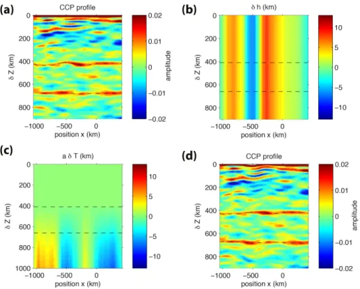
continuities and the velocity heterogeneities above the TZ. As depicted in
43
Fig. 1a, shallow velocity anomalies negatively correlated with the
temper-44
ature in the transition zone apparently enhance the ‘410’ topography and
45
reduce the ‘660’ topography (e.g. the case of a hot lithosphere on top of a
46
hot mantle, Fig. 1a, left, or reciprocally, right). Shallow velocity anomalies
47
positively correlated with the temperature in the transition zone could lead
48
to an overestimate of the ‘660’ topography compared to that of the ‘410’ (e.g.
49
a thin crust on top of a hotter mantle, Fig. 1b left, or reciprocally, right).
50
In general, the absence or the inaccuracy of velocity corrections obscure the
51
anti-correlation between the discontinuity depths (e.g. Stammler and Kind,
52
1992). In extreme cases where the contribution from shallow velocity
het-53
erogeneities exceeds the contribution from the temperature (i.e., all 4 cases
54
in Fig. 1), the topographies appear correlated and the apparent Clapeyron
55
slope ratio γ4/γ6 becomes positive, contrary to experimental expectations. 56
This could be especially the case for up-going P waves converted into shear
57
waves under seismological stations (P-to-S conversions) whose travel-times
58
are strongly velocity-dependent (Li et al., 2003).
59
In this study, we propose a method to separate the competing effects
60
of uppermost velocity structure and temperature on the topography of TZ
410 660 0
true depth apparent depth Low T High T Low Vp,s High Vp,s γ4 > 0 γ6 < 0 410 660 0 Low T High T High Vp,s Low Vp,s (a) (b)
δv and δT negatively correlated
δv and δT positively correlated
δv < 0 δv > 0 δT > 0 δT > 0 δv > 0 δT < 0 δv < 0 δT < 0
Figure 1: Behavior of discontinuities with thermal anomalies in the transition zone and strong velocity heterogeneities in the lithosphere. Topographies of opposite signs expected from mineral physics are shown with plain lines whereas seismological observations, influ-enced by the uppermost velocity structure, are shown with dashed lines. In the absence of shallow corrections, an apparent correlation between the interface topographies may be observed. (a) Case of a slower lithosphere on top of a hotter mantle (left) and reciprocally (right). (b) Case of a faster lithosphere (e.g. due to a thin crust) on top of a hotter mantle (left) and reciprocally (right).
discontinuities. This method makes possible the determination of the ratio
62
γ4/γ6 with little information on the background velocity structure. From this 63
estimate, we can correct the structure of the TZ from the effect of velocities,
64
estimate the temperature, and build diagrams that may be used as a proxy for
65
thermodynamics phase diagram of solid-solid transitions. Then we develop
66
and apply a new method, the “Z-Γ stacking”, to test the presence of unknown
67
phase transitions in the mantle and measure their relative Clapeyron slopes.
68
2. Seismic observations under Western US
69
We make use of a dataset of P-to-S conversions obtained from the
Trans-70
portable Array component of USArray. This dataset is described in detail
71
in Tauzin et al. (2013). Using receiver functions, the mantle structure of the
72
western half of the US (Fig. 2a) has been characterized in the 5-75 s period
73
range. Seismic images of mantle discontinuities have been produced by a
mi-74
gration method, stacking the receiver functions by common conversion point
75
(CCP) (Dueker and Sheehan, 1997; Wittlinger et al., 2004). The imaged
vol-76
ume is thus called a “CCP volume”. By picking in this volume the seismic
77
signal of conversions at the ‘410’ and ‘660’, high resolution maps of their
78
apparent topographies (δZ4 and δZ6) have been obtained on a 0.5◦ grid in 79
latitude and longitude (Fig. 2b,c). The observed average depths of the ‘410’
80
and ‘660’ over the area are < Z4 >= 424 km and < Z6 >= 676 km. The cor-81
responding peak-to-peak depth variations are 55 km for the ‘410’ and 49 km
82
for the ‘660’ (with RMS 9.8 km and 8.8 km, respectively). The migration
83
being performed using a spherical model, IASP91 (Kennett and Engdahl,
84
1991), the topography maps do not take into account lateral variations of
−4 km −2 km 0 2 km elevation (km) 125° W 120° W 115° W 110° W 105° W 35° N 40° N 45° N 50° N 125° W 120° W 115° W 110° W 105° W 35° N 40° N 45° N 50° N 125° W 120° W 115° W 110° W 105° W 35° N 40° N 45° N 50° N −25 −15 0 15 25 topography (km)
(a)
(b)
(c)
410-km 660-kmFigure 2: (a) Surface topography with state borders. (b) Apparent topography δZ4of the
‘410’ seismic discontinuity. (c) Apparent topography δZ6 of the ‘660’ discontinuity (both
panels from Tauzin et al., 2013).
velocities within the mantle. We thus expect shallow velocity heterogeneities
86
to significantly affect the apparent topography of TZ discontinuities.
87
Fig. 3 shows that this is indeed the case. Contrary to mineral physics
88
expectations, the ‘410’ and the ‘660’ topographies have a positive correlation
89
of +0.60 (Fig. 3a). This correlation is partly the result of shallow velocity
90
heterogeneities in the mantle overlying the TZ. The depth-velocity trade-off
91
is obvious by looking at average δvp anomalies above the TZ taken from 92
the tomographic model of Burdick et al. (2010), versus the ‘410’ topography
in Fig. 3b. The correlation is negative, -0.68, as a slower lithosphere tends
94
to increase the apparent depths of the discontinuities (see Fig. 1a left, and
95
Fig. 1b, right). This trade-off reduces slightly to -0.45 when examining the
96
‘660’ topography (Fig. 3c). Similar observations from SS-precursors have
97
already been discussed by Houser et al. (2008).
98
3. Clapeyron slopes of the ‘410’ and the ‘660’
99
3.1. Seismic imaging of discontinuities
100
We assume that at first order, the “depth variation” δZ of a phase
transi-101
tion depends on its Clapeyron slope, γ and on the temperature variations δT
102
(i.e. the temperature minus the adiabatic reference geotherm). The potentiel
103
effects of compositional heterogeneities (e.g., water content or variability in
104
Mg/Fe ratios, Litasov et al. (2005a); Irifune et al. (1998)) are considered as
105
second order effects. Depth and temperature are therefore related by
106
δZ = Z− < Z >= γ
ρgδT = ΓδT (1)
where g is Earth’s gravity, ρ the density above the discontinuity and Γ the
107
Clapeyron slope in m K−1 (while γ is in Pa K−1, see Helffrich and Bina
108
(1994)). The absolute depth of discontinuity Z and its average < Z >,
109
can be directly estimated from seismic imaging using for instance P-to-S
110
conversions (Tauzin et al., 2013) or SS-precursors (Houser et al., 2008). In
111
the case of our P-to-S observations, the travel times of converted waves Pds
112
relative to the direct P depend on the conversion depth Z, the ray parameter
113
p (assumed to be identical for the two waves), the S and P velocities vs, vp: 114 tP ds(p, Z) = Z Z 0 [pv−2 s − p2 − q v−2 p − p2] dz (2)
−40 −20 0 20 40 −1.5 −1 −0.5 0 0.5 1 1.5 C = −0.68 δ Z4 (km) 380 400 420 440 460 640 660 680 700 C = +0.60 ’410’ depth (km) ’660’ depth (km) (a) (b) (c) δ v p (%) −40 −20 0 20 40 −1.5 −1 −0.5 0 0.5 1 1.5 δ Z6 (km) δ v p (%) C = −0.45
Figure 3: (a) Observed ‘660’ depth Z6versus the ‘410’ depth Z4. The oblique dashed line
represents perfectly correlated topographies. (b) Average tomographic velocity anomalies δvp above the ‘410’ versus the ‘410’ topography δZ4. (c) Average tomographic velocity
anomalies δvp above the ‘660’ versus the ‘660’ topography δZ6. The tomographic model
is from Burdick et al. (2010). Correlation coefficients are indicated at the top. The two topographies appear positively correlated contrary to mineralogical expectations. Their negative correlations with the shallow velocity suggest a large effect of the shallow structure on the apparent depths of discontinuities.
Supposing vp and vs perfectly known, this equation enables the projection of 115
the amplitude measured at time tP ds on a seismogram at the “true” depth 116
Z (this is called time-to-depth conversion). A more sophisticated but
simi-117
lar approach for interface imaging is to backpropagate the seismic wavefield
118
recorded at the surface, with the expectation that the transposed wavefield
119
will focus at and therefore will highlight the sources of seismic scattering in
120
the subsurface (this is called migration; e.g., Rondenay, 2009).
121
However in these methods, the imperfect knowledge of the shallow
veloc-122
ity structure leads to an imperfect recovery of the interface positions. Instead,
123
one recovers an apparent topography:
124
δZ = Z− < Z >= ΓδT + δh (3)
The correction term δh integrates the effects on travel-times of 3D
hetero-125
geneities δvs,p (δv = v − vref) encountered along the ray paths and not taken 126
into account by the reference model. Instead of (2) what is really used is:
127 tP ds(p, Z) = Z Z+δh 0 [ q vsref −2− p2−qv pref −2− p2] dz (4)
where vsref and vpref are velocities in the Earth’s reference model used for 128
imaging. The deviations of velocities δvs,p from the reference model are thus 129
mapped into δh. Using (2), the latter identity can be used to express δh,
130
assuming a vertical incidence (p = 0):
131 δh = − RZ 0 [δvs/v 2 sref − δvp/v 2 pref] dz [1/vsref(Z) − 1/vpref(Z)] (5)
(practically, the P and S ray paths are not vertical so (5) is an
approxima-132
tion). In general δvs and δvp are correlated, and |δvs/vs2ref| > |δvp/v 2 pref|, 133
so that δh is anti-correlated with the seismic velocities above the TZ, i.e.
134
deeper interfaces δh > 0 are inferred for a slower lithosphere δvs,p < 0 (see 135
Fig. 1 and Fig. 3b,c).
136
The effect of δh can in principle be estimated from tomographic imaging.
137
However, the travel-time tomography is often resolved with longer
wave-138
lengths than what would be needed to accurately correct the local
infor-139
mation associated with converted/reflected body waves, especially at global
140
scale.
141
To alleviate the problem of mapping velocity variations into interface
142
topographies, various authors have discussed their results in term of TZ
143
thickness (e.g., Chevrot et al., 1999; Lawrence and Shearer, 2006; Tauzin
144
et al., 2008). Computing a difference of topographies cancels the major
145
corrections due to the shallow structure but leaves those due to the velocity
146
perturbations in between the two interfaces. For example, because of local
147
temperature variations, any possible interface within the TZ, appears shifted
148
with respect to the ‘410’, by the distance, see (5),
149 δhT(Z) = a(Z) δT = −K RZ Z4[1/vsref − 1/(Rvpref)] dz [1/vsref(Z) − 1/vpref(Z)] δT (6)
where the proportionality factor computed at the ‘660’ is a(< Z6 >) = 150
a6 = 0.03 km K−1 (using K = ∂ log vs/∂T = −7 10−5 K−1 (Stixrude and 151
Lithgow-Bertelloni, 2005) and R = ∂ log vs/∂ log vp = 2 (e.g., Schmandt and 152
Humphreys, 2010; Becker, 2011)). The contributions of the lateral
tempera-153
ture variations to the apparent thickness of the TZ are therefore non
negli-154
gible (3 km for 100 K) and a hotter TZ appears thicker without corrections.
3.2. Fundamental hypotheses
156
For the ‘410’ and the ‘660’ discontinuities, we suppose that the apparent
157
topographies are given by:
158
δZ4 = Γ4δT + δh
δZ6 = Γ6δT + δh + δhT(< Z6 >) = (Γ6+ a6) δT + δh = Γ06δT + δh
(7)
In the last equality we group together the two δT -dependent terms and define
159
an apparent Clapeyron slope Γ06 = Γ6 + a6. Equations (7) assume that the 160
temperature δT in the TZ does not vary with depth but uniquely laterally.
161
We will discuss this approximation in section 3.5.
162
The expectation from high pressure mineral physics is that Γ6/Γ4 < 0. 163
This effect alone imposes a negative correlation between δZ4 and δZ6 (see 164
(7)). On the contrary, the contribution of δh is opposite (see (7)). As a6 165
and Γ4 have the same sign, the temperature variations within the TZ also 166
tends to increase the correlation between the interfaces. The slight positive
167
correlation observed between the ‘410’ and ‘660’ topographies at a global
168
scale (Gu et al., 1998; Houser et al., 2008) could thus be partly explained by
169
an under-estimation of the velocity corrections.
170
3.3. The Clapeyron slope ratio and temperature in the TZ
171
Writing Γ4 δZ6 − Γ06 δZ4 (see (7)), we get the contribution from the 172
shallow heterogeneities as a function of an apparent Clapeyron slope ratio
173 (Γ06/Γ4) 174 δh = 1 1 − Γ06/Γ4 δZ6− 1 Γ4/Γ06− 1 δZ4 (8)
Our method considers the contribution δh as a noise to the real signal,
175
that must be minimized, i.e., we choose the Clapeyron ratio Γ06/Γ4 that 176
explains the ensemble of observations in terms of temperature variations
177
and shallow corrections, but requires the smallest shallow corrections. We
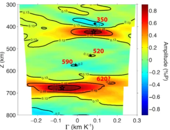
178
therefore look for the ratio Γ06/Γ4 that minimizes the quantity: 179
χ2 =< δh2 > (9)
We can show that an analytical solution to ∂χ/∂(Γ06/Γ4) = 0 is: 180 Γ06 Γ4 = < δZ6· (δZ6− δZ4) > < δZ4· (δZ6− δZ4) > (10)
The expression (10) can also be understood from a different standpoint.
181
The shallow corrections and the temperature in the transition zone are likely
182
uncorrelated on average. The shallow corrections are mostly due to crustal
183
anomalies and fossil structure of the lithosphere. Their correlation with the
184
thermal TZ structure is very low in global tomography models (see e.g.,
185
Becker and Boschi, 2002). We may therefore assume that the correlation
186
between δh and δT is zero, i.e < δT · δh >= 0. We discuss further the
187
validity of this assumption in the section 3.5. In this case, one has simply
188 from (7) 189 < δZ4· δZ4 >= Γ24 < δT · δT > + < δh · δh > < δZ6· δZ6 >= Γ 02 6 < δT · δT > + < δh · δh > < δZ6· δZ4 >= Γ4Γ06 < δT · δT > + < δh · δh > (11)
Subtracting the last equation to the first two and removing the term <
190
δT ·δT > by division, leads again to the relation (10). In conclusion, choosing
191
the Clapeyron slope ratio according to (10) simultaneously minimizes the
192
overall shallow corrections and their correlations with the TZ structure.
−108 −5 0 8.5 9 9.5 χ (km) Γ’6 / Γ4
Figure 4: The minimization of the shallow corrections (see (9)) occurs for Γ06/Γ4= −0.56.
The minimization process allows us to compute the ratio of the apparent
194
Clapeyron slopes, Γ06/Γ4 but not the two mineralogical Clapeyron slopes γ6 195
and γ4, independently. If one of the Clapeyron slope is known, e.g. at the 196
‘410’, then the Clapeyron slope of the ‘660’ is obtained from
197 γ6 = ρ6 ρ4 Γ06 Γ4 γ4− ρ6ga6 (12)
where ρ4 and ρ6 are the reference densities above the ‘410’ and ‘660’. 198
From δZ4− δZ6 (see (7)), we obtain the TZ temperature as: 199 δT = 1 Γ4 1 (1 − Γ06/Γ4) (δZ4− δZ6) (13)
The temperature field within the TZ is thus linearly related to the
vari-200
ations in TZ thickness. The thermal contributions to the ‘410’ topography,
201
i.e., Γ4δT , is obtained by our method but we must assume the independent 202
knowledge of one of the Clapeyron slope (e.g. Γ4) to obtain δT . 203
3.4. Application to western US
204
In the following, we use our observations of apparent topographies of TZ
205
discontinuities below western US to estimate the ratio of the ‘410’ and ‘660’
Clapeyron slopes. We plot in Fig. 4 the root mean square function χ(Γ06/Γ4) 207
(9) which goes through a minimum at (Γ06/Γ4) = −0.56, given, as expected, 208
by (10). We find no minima for positive values of (Γ06/Γ4). According to (12), 209
we therefore predict a relation between the mineralogical Clapeyron slopes
210
γ6 = −0.64 γ4− 1.17 (14)
where we used a6 = 0.030 km K−1, ρ4 = 3542 kg m−3, and ρ6 = 3991 kg m−3. 211
For γ4 = +3.0 MPa K−1, we obtain γ6 = −3.1 MPa K−1 and γ4/γ6 = −1.03. 212
We show in Fig. 5 the result of applying (13) with Γ06/Γ4 = −0.56 and 213
taking γ4 = +3.0 MPa K−1, close to the average of experimental values in 214
table S.1. As expected from equation (13), the pattern of thermal anomalies
215
is proportional to the TZ thickness (Tauzin et al., 2013). The choice of γ4 216
determines the range of thermal variations δT , from -259 K below northeast
217
Oregon to +216 K below Yellowstone, with a 65 K RMS (Fig. 5). This
218
temperature is weakly but positively correlated with what can be estimated
219
from tomography in the TZ (correlation of +0.23 with Burdick et al. (2010)’s
220
model at mid TZ).
221
In Fig. 6a, we plot a map of the depth corrections δh computed from
222
(8) and Γ06/Γ4 = −0.56. These corrections should represent the contribution 223
of shallow velocity heterogeneities to the interface topographies. A clear
224
NE-SW dichotomy is observed with δh values ranging from -25 km below
225
northern Idaho to +17 km in the southwest of Utah, with a RMS of 8.5 km.
226
This dichotomy dominates the initial maps of topographies (Fig. 2b,c).
227
The corrections δh can be compared with those, δhtomocomputed with the 228
P-wave model of Burdick et al. (2010) (Fig. 6b). To estimate δhtomo, a shear-229
wave model δvsis required (5). We scale δvsfrom δvp using δ log vs/δ log vp = 230
125° W 120° W 115° W 110° W 105° W 35° N 40° N 45° N 50° N −200 −100 0 100 200 δ T δT (K)
Figure 5: Map of temperature anomalies δT within the TZ obtained from (13) and γ4=
+3.0 MPa K−1.
2 (e.g., Romanowicz and Cara, 1980; Schmandt and Humphreys, 2010). This
231
value of δ log vs/δ log vp has no impact on the high correlation between δh and 232
δhtomo, +0.65. The amplitudes of δhtomo are generally lower than predicted 233
with our method (Fig. 6a) but the NE-SW dichotomy is well recovered. This
234
confirms the dominant effect of shallow velocities on the apparent
topogra-235
phies of TZ discontinuities.
236
The corrections δh and δh + a6δT must be removed from the observed to-237
pographies δZ4 and δZ6 to obtain the “true” topographies (7), perfectly anti-238
correlated by construction and due to temperature variations alone (Fig. 6c
239
and d). The estimated Clapeyron slope ratio γ6/γ4 being ∼-1.0, the relative 240
amplitudes of thermal topographies are similar. In term of RMS amplitudes
241
the initial topographies for the ‘410’ and ‘660’ are of 9.8 and 8.8 km, from
242
which we removed a shallow correction related to δh of 8.5 km, a temperature
243
correction at ‘660’ related to a6δT of 1.9 km, leaving thermal topographies 244
of 5.3 and 4.9 km respectively.
125° W 120° W 115° W 110° W 105° W 35° N 40° N 45° N 50° N −20 −10 0 10 20 δ h (km) 125° W 120° W 115° W 110° W 105° W 35° N 40° N 45° N 50° N −20 −10 0 10 20
(a)
δ h (km) δ htomo(b)
δ hobs depth (km) 125° W 120° W 115° W 110° W 105° W 35° N 40° N 45° N 50° N −20 −10 0 10 20(c)
`410’ depth (km)(d)
`660’Figure 6: (a) Map of the depth corrections δh obtained with the apparent Clapeyron slope ratio (Γ06/Γ4) = −0.56. (b) Map of the corrections δhtomo (5) computed with the
δvp model of Burdick et al. (2010) and R = ∂ ln vp/∂ ln vs = 2. (c) Map of the ‘410’
thermal topography Γ4δT . (d) Map of the ‘660’ thermal topography Γ6δT . The thermal
3.5. Critical assessment
246
Our method makes use of two hypotheses: a low correlation between the
247
shallow corrections and the temperature in the TZ and a TZ temperature
248
varying only laterally. These hypotheses allow us to correct the direct
obser-249
vations of interface topographies without using a tomographic model.
250
Our assumption of a weak correlation between the shallow correction and
251
the temperature in the TZ is in relative agreement with Burdick et al. (2010)’s
252
model where the shallowest 400 km (a proxy for shallow corrections) are
253
weakly correlated (-0.17) with the tomographic anomalies at 500 km (a proxy
254
for the TZ structure). In Supplement S.1, we discuss how this correlation
255
C(δh, δT ) may affect our results. When C(δh, δT ) varies from -0.2 to +0.2,
256
we show that the ratio Γ06/Γ4 derived from the data changes from -0.19 to 257
-1.23. The assumption of an uncorrelation between shallow corrections and
258
the TZ temperature is therefore crucial. Using the correlation value suggested
259
by Burdick’s mantle model would change our estimate for Γ06/Γ4from -0.56 to 260
-0.23, or using (14), our estimate of γ6 from -3.1 to -2.0 MPa K−1. Note that 261
crustal heterogeneities, which are not explicitly given in the mantle model of
262
Burdick et al. (2010) should rather decrease than increase |C(δh, δT )|. With
263
C(δh, δT ) = −0.17 the RMS thermal topography at ‘410’ slightly increases
264
from 5.3 to 6.2 km, that at ‘660’ decreases from 4.9 to 4.3 km, and the RMS
265
of the corrections δh does not change much with C(δh, δT ).
266
In Supplement S.2, we also discuss the assumption of a uniform
tem-267
perature in the TZ. We show that as soon as the RMS of the difference of
268
temperature between the two interfaces is lower than that of the lateral
vari-269
ations, the retrieved Γ06/Γ4 is not significantly affected. The fact that the 270
vertical difference of temperature in the 250 km thick TZ is not larger than
271
the horizontal temperature differences below western US seems reasonable.
272
Therefore, the accuracy of our method is mostly affected by the
assump-273
tion of an uncorrelation between surface corrections and the TZ temperature
274
and not much by the sampling of our dataset (we checked by bootstrap
re-275
sampling that similar results are obtained by using only subsets of our data)
276
or by the assumption of a vertically uniform TZ. Of course, if tomographic
277
models were extremely precise they could be used to correct the observations
278
or to check our hypotheses. Unfortunately, we consider that this appears
279
difficult even with high quality models like that of Burdick et al. (2010).
280
First, tomographic inversions involve smoothing and regularization that
281
limit their accuracy at the short length-scale at which interface topographies
282
are mapped by receiver functions. Second, velocity variations close to an
283
interface, can be interpreted as due to temperature variations in a medium
284
with flat interfaces or as due to interface undulations in a medium without
285
other velocity anomalies. In the first case we would assume that δvp/vp = 286
(∂ log vp/∂T ) δT ≈ −3.5 10−5δT . In the second case, an interface topography 287
δZ = ΓδT seen with a resolution λ would appear as an anomaly δvp/vp = 288
−(∆vp/vp)(Γ/λ) δT where ∆vp/vp is the velocity jump across the interface 289
(∆vp/vp ≈ 4% and 6% at the ‘410’ and ‘660’). We would obtain δvp/vp ≈ 290
− 5 10−5 δT near the ‘410’ and δv
p/vp ≈ +10 10−5 δT near the ‘660’ for 291
a resolution length of λ = 40 km. Of course a combination of the two
292
effects is likely. The above numerical applications imply that we may not
293
even know the sign of the temperature anomaly near the ‘660’ and that
294
accurate temperature estimate at ‘410’ is unlikely. It seems to us that unless
tomographic models are obtained by simultaneous inversion of both velocities
296
and interfaces (like e.g. in Gu et al., 2003; Houser et al., 2008; Lawrence and
297
Shearer, 2008, but with a better regional resolution), the estimate of TZ
298
temperatures from tomographic models with flat interfaces will introduce
299
more, or at least as much uncertainties as our simpler approach.
300
4. Phase changes in the transition zone
301
4.1. Seismically deduced phase diagrams
302
Now that we have estimated the velocity corrections and the TZ
temper-303
ature we can directly use the waveforms to construct a representation of the
304
thermodynamic phase diagram seen from seismology and to search for other
305
potential phase changes.
306
In Fig. 7a, we stack all the seismic signals si(Z) within intervals of appar-307
ent depths δZ4 of the ‘410’. The ‘410’ and the ‘660’ appear as well-resolved 308
streaks. The slopes of δZ4 and δZ6, both positive in this diagram, are con-309
trolled by shallow heterogeneities δh (see (7)). Their slight difference is due
310
to the weak expression of temperature.
311
A more meaningful observation of the interfaces is obtained by correcting
312
the traces from the shallow heterogeneities, hence by considering si(Z − δhi) 313
where δhi is given by (8) and (10). This is done in Fig. 7b, here as a function 314
of the thermal topography of the ‘410’, Γ4δT . The effect of the corrections 315
is drastic on the ‘660’, straightening it up to an opposite direction to that of
316
the ‘410’.
317
All the interfaces in the TZ are also displaced by a(Z) δT (see (6)). The
318
best representation of the effects of the temperature on phase changes is
−200 0 200 300 400 500 600 700 800 temperature anomaly (K) depth (km) ol wd rw pv+fp LVL olivine-wadsleyite transition ringwoodite-perovskite transition Mg-pv-in mj-out ak-in fp-in rw-out ak-Pv (a) (b) (c) (d) si(Z) si(Z- δhi) si(Z- δhi - a δTi)
Figure 7: (a) Diagram of the seismic signals si(Z) stacked within 2 km intervals of the
apparent depth of the ‘410’, δZ4. Positive amplitudes (in red) mark velocity increases with
depth whereas negative amplitudes (in blue) are associated with velocity reductions. The black line is the relation Z =< Z4 > +δZ4. (b) Diagram of si(Z − δhi), corrected from
shallow heterogeneities. The black line is the relation Z =< Z4 > +δZ4− δh =< Z4 >
+Γ4δT . (c) Seismic phase diagram F (Z, δT ) (using γ4= +3 MPa K−1 and stacking the
seismic signal by intervals of 20 K). (d) Our interpretation. ol: olivine; wd: wadsleyite; rw: ringwoodite; fp: ferropericlase; pv: perovskite; mj: majorite; ak: akimotoite. LVL: Low velocity layer atop the ‘410’. The phase diagram for transformations at the bottom of the transition zone is taken from Hirose (2002) for pyrolite. The dashed ellipse locates
obtained by plotting the function F (Z, δT ) (see Fig 7c) obtained by stacking
320
si(Z − hi− a(Z) δTi) as a function of δTi 321
F (Z, δT ) =< si(Z − hi− a(Z) δTi, δTi) > for δTi ≈ δT. (15)
The function F (Z, δT ) represents our best estimate of the position of the
322
interfaces as a function of temperature, what we call a “seismic phase
dia-323
gram”. Note that the construction of this diagram requires the choice of the
324
‘410’ Clapeyron slope to properly scale δT . Here we choose γ4 = +3.0 MPa 325
K−1. In this “seismic phase diagram” the phase changes at ’410’ and ’660’
326
are straight lines with slopes Γ4 and Γ6. Any other phase transformation ap-327
pears as a line of slope Γ. The ol→wd and rw→fp+pv are clearly visible but
328
the wd→rw transition is very faint (encircled by a dashed ellipse in Fig 7d).
329
Other signals in the diagram can either be associated with phase transitions
330
if they align on linear trends, or with “noise” if they do not, due for instance
331
to compositional effects.
332
This approach can also be used to correct seismic sections for the mantle
333
(see Fig. S.2). As an example, the initial section for a profile at 41◦N
334
is corrected from the shallow heterogeneity and the temperature induced
335
velocity changes and leads to a profile where the signal should be only due
336
to the true interface undulations.
337
Tauzin et al. (2013) reported the presence of seismic discontinuities around
338
350, 590 and 620 km depths in the mantle below western US. These features
339
are more local than the ‘410’ and ‘660’ but appear anyway in the diagram
340
of Fig 7c. For cold regions of the mantle (< −150 K of thermal anomaly), a
341
negative signal is observed atop the ‘410’ around 380 km depth (the ‘350’).
342
This same temperature domain is characterized by multiple positive peaks
above the ‘660’ and by what we can associate with a positive ‘620’
disconti-344
nuity. The negative signal of the ‘590’ is diffuse: it can be found across the
345
whole temperature range with higher amplitudes in the hottest environments
346
(dotted contour in Fig 7d). We checked by making seismic phase diagrams
347
restricted to the eastern or western regions relative to the Nevada/Utah
bor-348
ders, that the characteristics of our observations in Tauzin et al. (2013) are
349
preserved. We observe the ‘350’ in both eastern and western regions with
350
stronger amplitudes in the west, the negative ‘590’ mostly in the east, and
351
the positive ‘620’ in both areas. This confirms that these minor interfaces
352
are robust in their seismological observation.
353
The minor interfaces seem also consistent with our model of phase changes
354
and vertically coherent temperature in the TZ. They are not noise or
ran-355
dom scatterers because they are seen coherently in quite specific domains of
356
temperature in the diagram. Indeed, they do not appear as coherent as we
357
stack the data as a function of the apparent ‘410’ topography (see Fig 7a).
358
Their origin is thus likely related to the temperature in the TZ.
359
4.2. Z-Γ stacking for the Clapeyron slope of unknown phase transitions
360
This seismic phase diagram suggests a simple way to interrogate the data
361
for the presence of phase transitions in the mantle. We simply stack all
362
the observations, corrected from the velocity perturbations, along the lines
363
of slopes Γ. This method is akin to the slant stack τ -p method (Rost and
364
Thomas, 2002) or the more general Radon transform (Gu and Sacchi, 2009)
365
that sum up signals, not at constant depth (or time) but along a specific
integration path. We thus build a Z-Γ diagram G(Z, Γ),
367
G(Z, Γ) = Z
F (Z − ΓδT, δT ) dT (16)
This function (see Fig 8) presents two maxima at Z = 424 km and Γ =
368
+0.081 km K−1 for the ‘410’ and at Z = 677 km and Γ = −0.079 km K−1
369
for the ‘660’. Their Clapeyron slope ratio is close to the estimate of section
370
3.4 (here we compute the maximum of an average signal while in section 3.4
371
we compute the average of the positions of maxima: this explains the small
372
difference). As reported in Tauzin et al. (2013) the amplitudes of the signals
373
converted at the ‘410’ and ‘660’ are comparable (∼1% of the P signal) while
374
radial models (PREM or IASP91) would predict a 50% larger signal for the
375
conversion at the ‘660’ which suggests that radial models overestimate the
376
velocity jump at the ‘660’. Other maxima in the G(Z, Γ) diagram potentially
377
indicate the presence of additional phase transitions in the mantle near the
378
depth Z and with a Clapeyron slope Γ.
379
The additional minor seismic discontinuities reported in Tauzin et al.
380
(2013) and in Fig 7c are also present as weak local extrema in the Z-Γ domain
381
(small stars). The ‘350’ is recovered at 387 km depth with an apparent
382
Clapeyron slope Γ = +0.092 km K−1 and the ‘590’ at 573 km with Γ =
383
−0.010 km K−1. The two discontinuities have absolute amplitudes within 20 384
to 30% of the ‘410’ or ‘660’ amplitudes (i.e. ∼0.3% the P-wave amplitude).
385
A peak at Z = 530 km and Γ = +0.064 km K−1 could correspond to the
386
wd→rw transition but the signal is weak with an amplitude of only 0.1%
387
the P-wave (i.e. 14% the conversion at the ‘660’). The ‘620’ appearing
388
as a conspicuous feature in Fig 7c is not reliably constrained with our Z-Γ
389
stacking approach because it is close to the strong signal from the ‘660’.
Amplitude (%P) 350 520 590 620? Γ (km K-1)
Figure 8: Z-Γ diagram. The amplitudes are red (positive) for velocity increases and blue (negative) for velocity reductions. The stars correspond to the couples (< Z >, Γ) expected for the ‘410’ and ‘660’ and inferred for minor extrema that are found around 350, 520, 590 and 620 km depths.
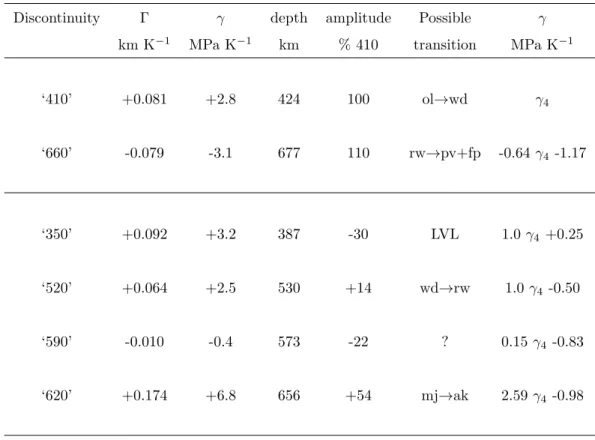
A summary of our results is given in table 1. In the second and third
391
columns Γ and γ assume γ4 = +3 MPa K−1. The depths reported in the 392
fourth column correspond to the potential depth of the interface in a
refer-393
ence mantle with zero thermal anomalies. For instance the ‘620’ which only
394
appears for δT ≈ −200 K is mentioned at a depth of 656 km in table 1
be-395
cause of its large Clapeyron slope, +0.174 km K−1 (‘620’ ≈ 656 − 0.174 × 200
396
km). For simplicity we mostly discussed our results assuming γ4 = +3.0 397
MPa K−1 but as explained in section 3 we can only derive linear relations
398
between Clapeyron slopes. In the last column of table 1 we report these
re-399
lations with respect to γ4 (the third column is in agreement with the last one 400
when γ4 = +3 MPa K−1). Ascribing uncertainties to these slopes is difficult. 401
However from the horizontal sizes of the extrema in Fig 8 the uncertainties
402
are probably as large as 0.02 km K−1 (≈0.7 MPa K−1).
Table 1: Summary of potential phase transitions observed in the TZ.
Discontinuity Γ γ depth amplitude Possible γ km K−1 MPa K−1 km % 410 transition MPa K−1
‘410’ +0.081 +2.8 424 100 ol→wd γ4 ‘660’ -0.079 -3.1 677 110 rw→pv+fp -0.64 γ4-1.17 ‘350’ +0.092 +3.2 387 -30 LVL 1.0 γ4 +0.25 ‘520’ +0.064 +2.5 530 +14 wd→rw 1.0 γ4 -0.50 ‘590’ -0.010 -0.4 573 -22 ? 0.15 γ4 -0.83 ‘620’ +0.174 +6.8 656 +54 mj→ak 2.59 γ4 -0.98 5. Conclusion 404
In this study, we used the competing actions of temperature and velocities
405
on the apparent topography of TZ discontinuities to quantify their respective
406
effects neglecting the possible presence of compositional variations. The
ex-407
pected anti-correlation of the ’410’ and ’660’ is largely hidden by the effects
408
of shallow velocity anomalies and the RMS thermal topographies (5.3 and
409
4.9 km) are lower than that of the corrections (8.5 km).
410
We suggest that the Clapeyron slope ratios of the two major interfaces of
the TZ can be obtained by minimizing the sallow corrections or by assuming
412
the absence of correlation between these corrections and the TZ
tempera-413
ture. The knowledge of the correlation between the TZ temperature and the
414
shallow corrections derived from tomography may be used to improve this
415
estimate (see Supplement S.1) but the exercise is not easy. This correlation
416
is an important parameter that impacts our ability to measure the exact
417
Clapeyron slopes of the ‘410’ and ‘660’. By comparison the other sources
418
of uncertainty, e.g., the lateral averaging in the migration process or the
419
assumption that the TZ temperature only varies laterally, seem to be less
420
crucial.
421
The presence of minor seismic discontinuities have been reported below
422
western US by e.g., Simmons and Gurrola (2000), Song et al. (2004), Vinnik
423
et al. (2010) Schmandt et al. (2011), and more recently Tauzin et al. (2013).
424
These interfaces are very weak and more visible at low temperatures. Two
425
interfaces seem to correspond to a velocity reduction, two interfaces to a
426
velocity increase. We suggest a new method to construct the phase diagram
427
directly from the seismic observations and, through a Z-Γ transform, we
428
estimate the Clapeyron slopes of the potential minor phase changes.
429
The sharp reduction of velocity at 350 km depth can hardly be explained
430
in term of a transition toward a higher pressure assemblage as it is associated
431
with a shear-wave velocity drop (∼-30% of the conversion amplitude at the
432
’410’). It has been proposed to mark the onset of a low-velocity layer atop
433
the ‘410’ due to dehydration-induced partial melting (Revenaugh and Sipkin,
434
1994). We preferentially find this layer in cold environments. It may be
435
induced by water rather released from subduction than upwelling from the
deeper mantle like in the transition zone water filter model of Bercovici and
437
Karato (2003). We find for this discontinuity a Clapeyron slope γ = +3.2
438
MPa K−1close to γ4 = +2.8 MPa K−1, which suggests that the two interfaces 439
may be intimately related.
440
The weak interface at ‘590’ (Tauzin et al., 2013) does not seem to vary
441
much with temperature, with a small Clapeyron slope of -0.4 MPa K−1. It
442
is also associated with a velocity reduction (-20% of the reflection amplitude
443
at the ’410’). Its origin remains mysterious.
444
The interfaces at 520 and 620 km depth being associated with increases of
445
velocity can be more easily related to pressure-induced phase changes. The
446
‘520’ is likely associated with the wadsleyite-ringwoodite transformation. Its
447
Clapeyron slope is negative and in agreement with laboratory experiments
448
(Suzuki et al., 2000). This signal is however very weak, only 10% of the
449
conversion amplitude at the ‘410’, and its detection is not very reliable. The
450
wd→rw transition is expected to be broader and with a smaller velocity jump
451
than that of the ol→wd transition so is less likely visible to converted phases
452
(Bina, 2003).
453
The ‘620’ discontinuity is found above the ‘660’ in the coldest part of
454
the seismic phase diagram. Due to its close proximity to the ‘660’ signal
455
we cannot reliably constrain its Clapeyron slope though it appears positive
456
and greater than that of the ‘410’ in Figs 7 and 8. Tauzin et al. (2013)
457
tentatively associated this discontinuity with the onset of stability field of
458
akimotoite MgSiO3 below the triple border between Washington, Oregon and 459
Idaho. The presence of akimotoite owing to cold slabs was also suggested by
460
Schmandt et al. (2012) on the basis of a positive vs gradient above the ‘660’. 461
The akimotoite is the product of a phase change of majorite in the garnet
462
component occurring for low temperatures at similar pressure ranges as the
463
rw→pv+mw transition (Hirose, 2002; Akaogi et al., 2002; Ishii et al., 2011).
464
The phase diagrams that we construct from seismic observations assume
465
that the effects of metastability (see e.g., Kirby et al., 1996) or compositional
466
variations (see e.g., Ricard et al., 2005) are negligible. Water, for instance,
467
would promote the uplift of the ‘410’ and the thickening of the TZ (Wood,
468
1995; Smyth and Jacobsen, 2006) and may bias our temperature estimates.
469
Other factors have also been suggested to add complexity to the temperature
470
response of the TZ. The Clapeyron slopes γ for any phase transition may
471
vary slightly with pressure and temperature. The ‘410’ broadens at low
472
temperature and eventually bifurcates into two different transitions at lowest
473
temperature when olivine transforms to ringwoodite rather than wadsleyite
474
(Bina, 2003). These complexities do not seem to affect our seismic phase
475
diagram where the ‘410’ transition remains simple (albeit preceded by the
476
sharp ‘350’ velocity reduction at low temperature). The ‘660’ seems to be
477
thicker both at low and high temperature. This behavior is in agreement
478
with experimental phase diagrams (Hirose, 2002; Bina, 2003) where in cold
479
situation the akimotoite phase may form before the ringwoodite while at high
480
temperature the garnet phase transforms after the ringwoodite.
481
In conclusion, our method for computing the seismic phase diagrams and
482
estimating the Clapeyron slopes through the “Z-γ stacking” approach, is
483
easy to implement. It can be applied at a much larger scale, e.g, on global
484
datasets of P-to-S conversions (Tauzin et al., 2008), or on other global seismic
485
data such as precursors of S waves reflected halfway between sources and
receivers. We also plan to develop the same approach in different frequency
487
bands which should help to further refine the gradients of velocities in the
488
TZ and our knowledge of the phase transitions in the mantle.
489
490
Acknowledgments
491
492
We thank Jean-Philippe Perillat, two anonymous reviewers, and the
ed-493
itor, for the suggestions to improve the method and the manuscript. This
494
work was supported by a Chaire d’Excellence Fellowship from CNRS. We
495
thank the IRIS data center for providing seismological data.
496
References
497
Akaogi, M., Ito, E., 1993. Refinement of enthalpy measurement of MgSiO3 498
perovskite and negative pressure-temperature slopes for
perovskite-499
forming reactions. Geophys. Res. Lett. 20, 1839–1842.
500
Akaogi, M., Ito, E., Navrotsky, A., 1989. Olivine-modified spinel-spinel
tran-501
sitions in the system Mg2SiO4-Fe2SiO4: Calorimetric measurements, ther-502
mochemical calculation, and geophysical application. J. Geophys. Res. 94.
503
Akaogi, M., Ross, N., Mc Millan, P., Navrotsky, A., 1984. The Mg2SiO4 504
polymorphs (olivine, modified spinel an spinel). Thermodynamic
proper-505
ties from oxyde melt solution calorimetry, phase relations and models of
506
lattice vibrations. Am. Mineral. 69, 499.
507
Akaogi, M., Tanaka, A., Ito, E., 2002. Garnet-ilmenite-perovskite transitions
508
in the system Mg4Si4O12-Mg3Al2Si3O12at high pressures and high temper-509
atures: phase equilibria, calorimetry and implications for mantle structure.
510
Phys. Earth Planet. Inter. 132, 303–324.
511
Akaogi, M., Tanaka, A., Ito, E., 2007. Low-temperature heat capacities,
512
entropies and enthalpies of Mg2SiO4 polymorphs, and αβγ and post-spinel 513
phase relations at high pressure. Phys Chem Minerals 34, 169–183.
514
Becker, T., 2011. On recent seismic tomography for the western united states.
515
Geochem. Geophy. Geosys. 13, 1–11.
516
Becker, T., Boschi, L., 2002. A comparison of tomographic and geodynamic
517
mantle models. Geochem. Geophy. Geosys. 3, 1–48.
518
Bercovici, D., Karato, S., 2003. Whole mantle convection and transition-zone
519
water filter. Nature 425, 39–44.
520
Bina, C., 2003. Seismological constraints upon mantle composition. In:
Carl-521
son, R. (Ed.), Treatise on Geochemistry, vol. 2. Elsevier Science Publishing,
522
pp. 39–59.
523
Bina, C., Helffrich, G., 1994. Phase transition Clapeyron slopes and
transi-524
tion zone seismic discontinuity topography. J. Geophys. Res. 99, 15,853–
525
15,860.
526
Burdick, S., Hilst, R., Vernon, F., Martynov, V., Cox, T., Eakins, J., Karasu,
527
G., Tylell, J., Astiz, J., Pavlis, G., 2010. Model update january 2010:
Up-528
per mantle heterogeneity beneath north america from traveltime
tomogra-529
phy with global and usarray transportable array data. Seis. Res. Lett. 81,
530
689–693.
Chevrot, S., Vinnik, L., Montagner, J., 1999. Global-scale analysis of the
532
mantle Pds phases. J. Geophys. Res. 101, 20,203–20,219.
533
Chopelas, A., 1991. Thermal properties of β-Mg2SiO4 at mantle pressures 534
and pressures derived from vibrational spectroscopy: Implications for the
535
mantle at 400 km depth. J. Geophys. Res. 96, 11817–11829.
536
Chopelas, A., Boehler, R., Ko, T., 1994. Thermodynamics of γ-Mg2SiO4 537
from Raman spectroscopy at high pressure: the Mg2SiO4 phase diagram. 538
Phys. Chemistry of Minerals 21, 351–359.
539
Deuss, A., 2007. Seismic observations of transition zone discontinuities
be-540
neath hotspot locations. In: Foulger, G., Jurdy, D. (Eds.), Plates, Plumes,
541
and Planetary Processes. Geological Society of America.
542
Dueker, K., Sheehan, A., 1997. Mantle discontinuity structure from
mid-543
point stacks of converted P to S waves across the Yellowstone Hotspot
544
Track. J. Geophys. Res. 102, 8313–8327.
545
Fei, Y., Van Orman, J., Li, J., van Westrenen, W., Sanloup, C., Minarik,
546
W., Hirose, K., Komabayashi, T., Walter, M., Funakoshi, K., 2004.
Ex-547
perimentally determined postspinel transformation boundary in Mg2SiO4 548
using MgO as an internal pressure standard and its geophysical
implica-549
tions. J. Geophys. Res. 109.
550
Gu, Y., Dziewonski, A., Agee, C., 1998. Global de-correlation of the
topogra-551
phy of transition zone discontinuities. Earth Planet. Sci. Lett. 157, 57–67.
Gu, Y., Dziewonski, A., Ekstrom, G., 2003. Simultaneous inversion for
man-553
tle shear velocity and topography of transition zone discontinuities.
Geo-554
phys. J. Int. 154, 559–583.
555
Gu, Y., Sacchi, G., 2009. Radon transform methods and their applications
556
in mapping mantle reflectivity structure. Surv. Geophys. 30, 327–354.
557
Helffrich, G., 2000. Topography of the transition zone seismic discontinuities.
558
Rev. Geoph. 38, 141–158.
559
Helffrich, G., Bina, C., 1994. Frequency dependence of the visibility and
560
depths of the mantle discontinuities. Geophys. Res. Lett. 21, 2613–2616.
561
Hirose, K., 2002. Phase transitions in pyrolitic mantle around 670-km depth:
562
Implications for upwelling of plumes from the lower mantle. J. Geophys.
563
Res. 107.
564
Houser, C., Masters, G., Flanagan, M., Shearer, P., 2008. Determination and
565
analysis of long-wavelength transition zone structure using SS precursors.
566
Geophys. J. Int. 174, 178–194.
567
Houser, C., Quentin, W., 2010. Reconciling Pacific 410 and 660 km
discon-568
tinuity topography, transition zone shear velocity patterns, and mantle
569
phase transitions. Earth Planet. Sci. Lett. 296, 255–266.
570
Irifune, T., Kubo, N., Isshiki, M., Yamasaki, Y., 1998. Phase transformations
571
in serpentine and transportation of water into the lower mantle. Geophys.
572
Res. Lett. 25, 203–206.
Ishii, T., Kojitani, H., Akaogi, M., 2011. Post-spinel transitions in
pyro-574
lite and Mg2Sio4 and akimotoite-perovskite transition in MgSiO3: Precise
575
comparison by high-pressure high-temperature experiments with
multi-576
sample cell technique. Earth Planet. Sci. Lett. 309, 185–197.
577
Ito, E., Akaogi, M., Topor, L., Navrotsky, A., 1990. Negative
pressure-578
temperature slopes for reactions forming MgSiO3perovskite from calorime-579
try. Science 249, 1275.
580
Ito, E., Takahashi, E., 1989. Postspinel transformations in the system
581
Mg2SiO4-Fe2SiO4 and some geophysical implications. J. Geophys. Res. 94, 582
10,637–10,646.
583
Ito, E., Yamada, H., 1982. Stability relations of silicate spinels, ilmenite
584
and perovskites. In: Akimoto, S., Manghnanni, M. (Eds.), High-pressure
585
research in mineral physics. Center for Academic Publishing, Tokyo, pp.
586
405–419.
587
Katsura, T., Ito, E., 1989. The system Mg2SiO4-Fe2SiO4 at high pressures 588
and temperatures: precise determination of stabilities of olivine, modified
589
spinel and spinel. J. Geophys. Res. 94, 15,663–15,670.
590
Katsura, T., Yamada, H., Nishikawa, O., Song, M., Kubo, A., Shinmei,
591
T., Yokoshi, S., Aizawa, Y., Yoshino, T., Walter, M., Ito, E., Funakoshi,
592
K., 2004. Olivine-wadsleyite transition in the system (Mg,Fe)2SiO4. J.
593
Geophys. Res. 109, 1–12.
594
Katsura, T., Yamada, H., Shinmei, T., Kubo, A., Ono, S., Kanzaki, M.,
595
Yoneda, A., Walter, M., Ito, E., Urakawa, S., Funakosji, K., Utsumi, W.,
2003. Post-spinel transition in Mg2SiO4 determined by high P-T in situ 597
X-ray diffractometry. Phys. Earth Planet. Inter. 136, 11–24.
598
Kennett, B., Engdahl, E., 1991. Travel times for global earthquake location
599
and phase identification. Geophys. J. Int. 105, 429–465.
600
Kirby, S., Stein, S., Okal, E., Rubie, D., 1996. Metastable mantle phase
601
transformations and deep earthquakes in subducting oceanic lithosphere.
602
Rev. Geoph. 34, 261–306.
603
Lawrence, J., Shearer, P., 2006. A global study of transition zone thickness
604
using receiver functions. J. Geophys. Res. 111.
605
Lawrence, J., Shearer, P., 2008. Imaging mantle transition zone thickness
606
with SdS-SS finite-frequency sensitvity kernels. Geophys. J. Int. 174, 143–
607
158.
608
Lebedev, S., Chevrot, S., van der Hilst, R., 2002. Seismic evidence for olivine
609
phase changes at the 410- and the 660-kilometers discontinuities. Science
610
296, 1300–1302.
611
Li, X., Kind, R., Yuan, X., Sobolev, S., Hanka, W., Ramesh, D., Gu, Y.,
612
Dziewonski, A., 2003. Seismic observation of narrow plumes in the oceanic
613
upper mantle. Geophys. Res. Lett. 30, 1334.
614
Litasov, K., Ohtani, E., Sano, A., Suzuki, A., 2005a. Wet subduction versus
615
cold subduction. Geophys. Res. Lett. 32, 1–5.
616
Litasov, K., Ohtani, E., Sano, A., Suzuki, A., Funakoshi, A., 2005b. In situ
617
x-ray diffraction study of post-spinel transformation in a peridotite mantle:
Implication for the 660-km discontinuity. Earth Planet. Sci. Lett. 238, 311–
619
328.
620
Revenaugh, J., Sipkin, S., 1994. Seismic evidence for silicate melt atop the
621
410-km mantle discontinuity. Nature 369, 474–476.
622
Ricard, Y., Mattern, E., Matas, J., 2005. Synthetic Tomographic Images of
623
Slabs from Mineral Physics. In: van der Hilst, R., Bass, J., Matas, J.,
624
Trampert, J. (Eds.), Earth’s Deep Interior: Structure, Composition, and
625
Evolution. Vol. 160. American Geophysical Union, Washington, D.C., pp.
626
283–300.
627
Romanowicz, A., Cara, M., 1980. Reconsideration of the relation between S
628
and P station anomalies in North America. Geophys. Res. Lett. 7, 417–420.
629
Rondenay, S., 2009. Upper mantle imaging with array recordings of converted
630
and scattered teleseismic waves. Surv. Geophys. 30, 377–405.
631
Rost, S., Thomas, C., 2002. Array seismology: Methods and applications.
632
Rev. Geoph. 40, 1–27.
633
Schmandt, B., Dueker, K., Hansen, S., Jasbinsek, J., Zhang, Z., 2011. A
spo-634
radic low-velocity layer atop the western U.S. mantle transition zone and
635
short-wavelength variations in transition zone discontinuities. Geochem.
636
Geophy. Geosys. 12, 1–26.
637
Schmandt, B., Dueker, K., Humphreys, E., Hansen, S., 2012. Hot mantle
638
upwelling across the 660 beneath Yellowstone. Earth Planet. Sci. Lett.
639
331-332, 224–236.
Schmandt, B., Humphreys, E., 2010. Complex subduction and small-scale
641
convection revealed by body-wave tomography of the western united states
642
upper mantle. Earth Planet. Sci. Lett. 297, 435–445.
643
Shearer, P., 1991. Constraints on Upper Mantle Discontinuities From
Obser-644
vations of Long-Period Reflected and Converted Phases. J. Geophys. Res.
645
96, 18,147–18,182.
646
Shearer, P., 2000. Upper mantle seismic discontinuities. In: et al., S. K. (Ed.),
647
Earth’s Deep Interior: Mineral Physics and Tomography From the Atomic
648
to the Global Scale, Geophys. Monogr. Ser. Vol. 117. AGU, Washington,
649
D.C., pp. 115–131.
650
Simmons, N. A., Gurrola, H., 2000. Multiple seismic discontinuities near the
651
base of the transition zone in the Earth’s mantle. Nature 405, 559–562.
652
Smyth, J., Jacobsen, S., 2006. Nominally anhydrous minerals and Earth’s
653
deep water cycle. In: Jacobsen, S., van der Lee, S. (Eds.), Earth’s deep
654
water cycle. Vol. 167. AGU monograph, pp. 1–9.
655
Song, T., Helmberger, D., Grand, S., 2004. Low-velocity zone atop the
410-656
km seismic discontinuity in the northwestern United States. Nature 427,
657
530–533.
658
Stammler, K., Kind, R., 1992. Comment on “Mantle Layering from ScS
659
Reverberations, 2, the Mantle Transition Zone” by Justin Revenaugh and
660
Thomas H. Jordan. J. Geophys. Res. 97, 17,547–17,548.
661
Stixrude, L., Lithgow-Bertelloni, C., 2005. Mineralogy and elasticity of the
oceanic upper mantle: Origin of the low-velocity zone. J. Geophys. Res.
663
110.
664
Suito, K., 1977. High Pressure Research. Academic. N. Manghani and S.
Aki-665
moto.
666
Suzuki, A., Ohtani, E., Morishima, H., Kubo, T., Kanbe, Y., T., K., Okada,
667
T., Terasaki, H., Kato, T., Kikegawa, T., 2000. In situ determination of
668
the phase boundary between Wadsleyite and Ringwoodite in Mg2SiO4. 669
Geophys. Res. Lett. 27, 803–806.
670
Tauzin, B., Debayle, E., Wittlinger, G., 2008. The mantle transition zone as
671
seen by global pds phases : no clear evidence for a thin transition zone
672
beneath hotspots. J. Geophys. Res. 113.
673
Tauzin, B., van der Hilst, R., Wittlinger, G., Ricard, Y., 2013. Multiple
674
transition zone seismic discontinuities and low velocity layers below
west-675
ern United States. J. Geophys. Res.
676
Vinnik, L., Ren, Y., Stutzmann, E., Farra, V., Kiselev, S., 2010.
Observa-677
tions of S410p and S350p phases at seismograph stations in california. J.
678
Geophys. Res. 115, 1–12.
679
Wittlinger, G., Vergne, J., Tapponnier, P., Farra, V., Poupinet, G., Jiang,
680
M., Su, H., Herquel, G., Paul, A., 2004. Teleseismic imaging of subducting
681
lithosphere and moho offsets beneath western Tibet. Earth Planet. Sci.
682
Lett. 221, 117–130.
683
Wood, B., 1995. The effect of H2O on the 410-kilometer seismic discontinuity. 684
Science 268, 74–76.
S. Supplements
686
S.1. Effect of a correlation between δh and δT
687
Contrary to the situation in section 3.3, we assume here that there is a
688
correlation C between the temperature in the TZ, δT , and the corrections
689
due to shallow velocity anomalies, δh. Thus C =< δT · δh > /(∆T ∆h) is
690
non zero (where ∆T and ∆h are the RMS of δT and δh). The equations (11)
691 become 692 < δZ4· δZ4 >= Γ24∆T 2+ ∆h2+ 2Γ 4C∆T ∆h < δZ6· δZ6 >= Γ 02 6∆T 2+ ∆h2+ 2Γ0 6C∆T ∆h < δZ6· δZ4 >= Γ4Γ06∆T 2+ ∆h2+ (Γ 4+ Γ06)C∆T ∆h (S.1)
These three equations can be solved for the three unknowns ∆T , ∆h and
693
Γ06 when Γ4and C are given. The algebra is cumbersome but straightforward. 694
The solution Γ06/Γ4 as a function of C is plotted in Fig. S.1a. The solution 695
discussed in the main text corresponds to the case C = 0 (black star). Our
696
estimate remains correct when the correlation between the shallow correction
697
and the TZ temperature is weak (Fig. S.1a). We found also that the RMS
698
of the shallow correction δh (not shown here) is minimum when C = 0 and
699
vary only by ≈ 2% for −0.2 < C < 0.2. Also, the thermal topography at
700
‘410’ decreases rather linearly with C.
701
S.2. Effect of a vertical temperature gradient in the TZ
702
We assume now that the temperatures at the top and bottom of the TZ
703
differ by θ so that the temperature at the ‘660’ is δT + δθ/2 and at the ‘410’
704
is δT − δθ/2. Assuming that δh, δT and δθ (of RMS ∆θ) are uncorrelated,
−0.2 −0.1 0 0.1 0.2 −2.5 −2 −1.5 −1 −0.5 0 C(δ h, δ T) Γ’6 / Γ4 0 50 100 −2.5 −2 −1.5 −1 −0.5 0 θ (K) Γ’6 / Γ4 (a) (b)
Figure S.1: (a) Recovery of the Clapeyron slope ratio when varying the correlation C between δh and δT . The solution discussed in the main text is Γ06/Γ4= −0.56 for C = 0
(black star). (b) Sensitivity of the Clapeyron slope ratio when varying the RMS of the difference in temperature at the ‘410’ and ‘660’. The solution discussed in the text is Γ06/Γ4= −0.56 for θ = 0 K (black star).
the equations (11) become
706 < δZ4· δZ4 >= Γ24∆T 2+ ∆h2+ Γ2 4∆θ 2/4 < δZ6· δZ6 >= Γ 02 6∆T 2+ ∆h2+ Γ02 6∆θ 2/4 < δZ6· δZ4 >= Γ4Γ06∆T 2+ ∆h2− Γ 4Γ06∆θ 2/4 (S.2)
Again, these three equations can be solved for the three unknowns ∆T ,
707
∆h and Γ06 when Γ4 and ∆θ are given. The solution Γ06/Γ4 as a function of 708
∆θ is plotted in Fig. S.1a where we see that Γ06/Γ4 is not drastically affected 709
by the assumption used in the main text of ∆θ = 0.