Doppler shifts in the KATRIN experiment

Doppler Shifts in the KATRIN Experiment

by

Matthew K. Heine

Submitted to the Department of Physics

in partial fulfillment of the requirements for the degree of

Bachelor of Science in Physics

at the

MASSACHUSETTS INSTITUTE OF TECHNOLOGY

June 2008

@Matthew K. Heine All Rights Reserved

Author ...-

....

.

Department of Physics

May 9, 2008

Certified by...

Joseph Formaggio

kssistant Professor

Thesis Supervisor

A A

Accepted by. ...

David Pritchard

Chairman, Department Thesis Committee

MASSACHUSETTS INSTITUTE OF TECHNOLOGy

JUN 1R3 2008

A.

LIBRARIES

Doppler Shifts in the KATRIN Experiment

by

Matthew K. Heine

Submitted to the Department of Physics on May 9, 2008, in partial fulfillment of the

requirements for the degree of Bachelor of Science in Physics

Abstract

In the past few decades, neutrinos, which are predicted to be massless particles by the Standard Model of Particle Physics, have been shown to have non-zero mass. The absolute scale of this neutrino mass has significant implications in particle physics, astrophysics, and cosmology. The KATRIN experiment is designed to measure this absolute scale by examining the beta decay spectrum of molecular, gaseous tritium source. In this thesis, the beta decay of this molecular tritium is simulated to study the effects of "Doppler shifts" in the energy of the emitted electrons due to the random thermal motion and fluid flow velocity of the differentially pumped tritium gas. Simulated spectra are presented for three different neutrino masses and the relative effects of the thermal and flow velocities are discussed.

Thesis Supervisor: Joseph Formaggio Title: Assistant Professor

Acknowledgments

I would like to thank Asher Kaboth for allowing me to use his fitter, and for all the time and effort he invested into adapting his fitter for my purposes and getting it running. I would also like to thank him for his generous help throughout the project. I would like to thank Sarah Trowbridge for her efforts and assistance during this project. Furthermore, I would like to thank Professor Felix Sharipov for his very helpful and timely correspondences and for sending me data. And last, but not least, I would like to thank Professor Joseph Formaggio for giving me the opportunity to work on this project and to see the experiment in person.

Contents

1 Massive Neutrinos

1.1 The Discovery of the Neutrino ...

1.2 Motivation for a Non-Zero Neutrino Mass: Neutrino Oscillations . ..

1.3 The Impact of the Neutrino Mass Scale ...

2 The KATRIN Experiment

2.1 The Theory ...

2.2 The Status of Neutrino Mass Determination . 2.3 Advantages of KATRIN ...

2.4 The KATRIN Setup ... 2.4.1 Experimental Overview ... 2.4.2 The WGTS in Detail ...

3 Beta Decay

3.1 Fermi's Golden Rule ... 3.2 Tritium Beta Decay ... 3.3 The Fermi Function ... 3.4 The Kurie Plot ...

3.5 Molecular Decay and Final State Distribution

4 Thermal Motion and Doppler Shifts 5 Velocity Profile Due to Pumping

5.1 The Density/Pressure Profile ...

21 . . . .. .. . . . .. 21 . . .. . .. . . .. . 23 . .. . . .. . . .. . 24 . .. . .. . . .. . . 25 . .. . . .. . . .. . 26 . .. . .. . . .. . . 29 31 . . . .. . .. . . .. 31 . . .. . . .. . .. . 32 . . .. . .. . . .. . 33 . .. . . .. . . .. . 35 . .. . . .. . .. . . 37

5.2 The Viscosity of Tritium . . . ... 5.3 The Velocity Profile ...

5.3.1 The Navier-Stokes Equation . . . . 5.3.2 The Boltzmann Transport Equation .. 5.3.3 Boundary Conditions . . . .

6 Results & Analysis

6.1 The Density and Velocity Profiles . . . . 6.2 The Beta Spectra ...

6.2.1 Inclusion of the Final State Distribution 6.2.2 Interpretation of These Results . . . . . 6.3 The Integrated Spectra and Fit Results . . . . .

7 Conclusions A Simulation Code 57 . . . . . . 57 . . . . .. . .. . . . 57 . . . . . 59 . . . . . 66 . . . . . 68

List of Figures

1-1 The Beta Decay Spectrum of molecular tritium, T2. Note that this inuous energy spectrum is inconsistent with momentum/energy con-servation in a 2-body decay. This histogram was constructed from the stationary decay data in Fig. 6.2.1 and so, corresponds to a electron antineutrino mass of leV/c2 . . . .. . . ₁₄ 1-2 The impact of the neutrino mass scale on the question of hierarchical or

degenerate neutrino masses. Plotted are the neutrino mass eigenvalues (ml<m2<m3) as a function of the value of the lightest eigenvalue, ml. One can see that a positive identification of a neutrino mass above - 0.1eV would clearly indicate a quasi-degenerate mass scheme, whereas a positive identification of a neutrino mass below - 0.1eV would clearly indicate a hierarchical mass scheme. [6] . . . . 19

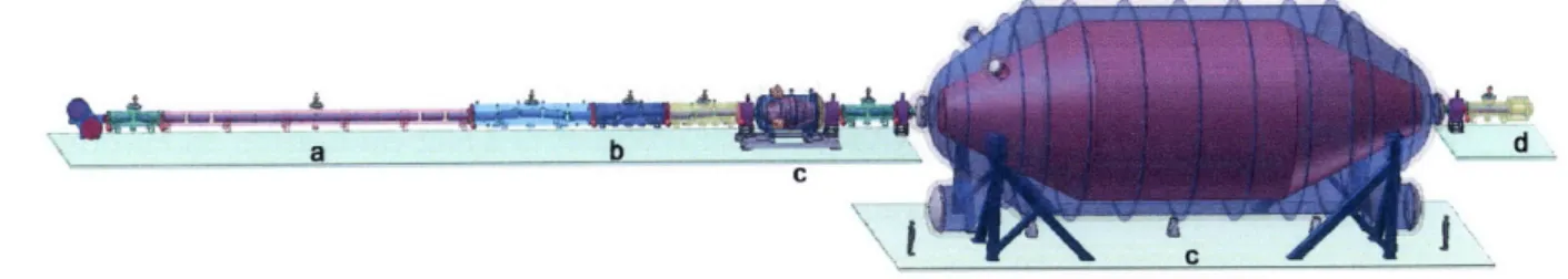
2-1 KATRIN Experimental Setup. a) the WGTS, b) the transport system, c) the spectrometers, d) the beta detector. Printed from [6] . . . . . 25 2-2 The Windowless Gaseous Tritium Source (WGTS) and Pumping

Sec-tions. Printed from [6] ... 28 2-3 The WGTS coordinate system used in this thesis . . . . 30

3-1 Beta Decay Spectra and corresponding Kurie Plots for stationary (in the rest frame of the decay) T2 decay for m,, = 1 and 0 eV/c2. Note

that, for m,, = 0, the Kurie plot is a straight line, whereas the Kurie plot for mi, = 1 eV/c2 dips near the endpoint. This figure is constructed from the same stationary decay data sets as in Figs. 6.2.1-6.2.1. . . . 36

3-2 The distribution of final states of the (3HeT)+, constructed from Eq.

3.13 and the data given in 3.12 . ... .. 39 5-1 Scaled Density/Pressure profile. This plot was constructed from the

data from Ref. [10, 21] .. ... .. 49

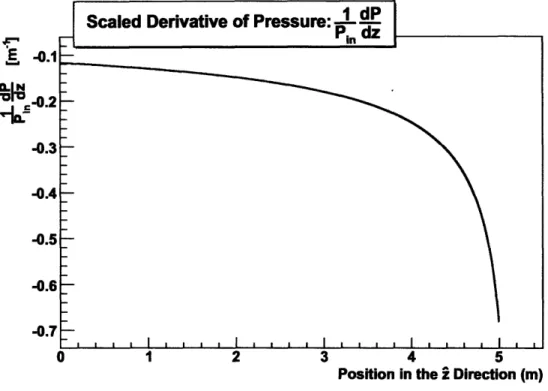
6-1 Scaled z derivative of Pressure. This plot was constructed by using a

spline interpolator tool with the data corresponding to Fig. 5.1. . .. 58 6-2 The flow velocity for tritium gas in the WGTS given by Eq. 5.28,

evaluated at z = L/4, where L is the length of the WGTS . . . . 58 6-3 A scatter plot of the distribution of particles within our 2D slice of the

W GTS. ... ... ... 59

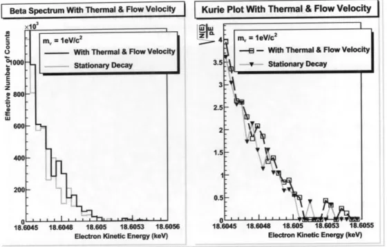
6-4 For a neutrino mass of leV/c2_{, the distortion of the beta spectrum,} and corresponding Kurie plot, due to the influenced of thermal motion, flow velocity, and the final state distribution. These beta specra were constructed with 5 - 109 decay events. . ... ... 60 6-5 For a neutrino mass of 0eV/c 2_{, the distortion of the beta spectrum,}

and corresponding Kurie plot, due to the influenced of thermal motion, flow velocity, and the final state distribution. These beta specra were constructed with 5 109 decay events . ... ... . 61 6-6 For a neutrino mass of leV/c2_{, the distortion of the beta spectrum,}

and corresponding Kurie plot, due to the influenced of thermal motion only. These beta specra were constructed via 7 - 109 _{decay events. . . 61}

6-7 For a neutrino mass of leV/c2_{, the distortion of the beta spectrum,} and corresponding Kurie plot, due to the influenced of the flow velocity only. Note that the scale of the energy axis of this figure is an order of magnitude less than the other figures considered in this section. These beta specra were constructed via 7 - 109 _{decay events . . . . 62}

6-8 For a neutrino mass of leV/c2_{, the distortion of the beta spectrum,} and corresponding Kurie plot, due to the influenced of both thermal motion and the flow velocity. This is the result of direct simulations of the two simultaneous effects, and was not obtained by simply adding Fig. 6.2.1 and Fig. 6.2.1. These beta specra were constructed via

7.-10 decay events ... 62 6-9 For a neutrino mass of 0.25eV/c 2_{, the distortion of the beta spectrum,}

and corresponding Kurie plot, due to the influenced of thermal motion only. These beta specra were constructed via 7. 109 decay events. . . 63 6-10 For a neutrino mass of 0.25eV/c2_{, the distortion of the beta spectrum,}

and corresponding Kurie plot, due to the influenced of the flow velocity only. Note that the scale of the energy axis of this figure is an order of magnitude less than the other figures considered in this section. These beta specra were constructed via 7 -10' decay events . . . . 63

6-11 For a neutrino mass of 0.25eV/c 2_{, the distortion of the beta spectrum,}

and corresponding Kurie plot, due to the influenced of both thermal motion and the flow velocity. Again, this is the result of direct simula-tions of the two simultaneous effects, and was not obtained by simply adding Fig. 6.2.1 and Fig. 6.2.1. These beta specra were constructed via 7.-109 _{decay events...}

64

6-12 For a neutrino mass of 0eV/c2_{, the distortion of the beta spectrum,}

and corresponding Kurie plot, due to the influenced of thermal motion only. These beta specra were constructed via 7. 109 decay events. . . 64 6-13 For a neutrino mass of 0eV/c2_{, the distortion of the beta spectrum,}

and corresponding Kurie plot, due to the influenced of the flow velocity only. Note that the scale of the energy axis of this figure is an order of magnitude less than the other figures considered in this section. These beta specra were constructed via 7 -109 _{decay events . . . . 65}

6-14 For a neutrino mass of 0eV/c2, the distortion of the beta spectrum, and corresponding Kurie plot, due to the influenced of both thermal motion and the flow velocity. Again, this is the result of direct simulations of the two simultaneous effects, and was not obtained by simply adding Fig. 6.2.1 and Fig. 6.2.1. These beta specra were constructed via

7. -109 decay events .. ... . 65

6-15 The integrated spectra for a neutrino mass of 0.25eV/c2. This figure is simply given as a representative example of the spectra over the entire range that KATRIN will measure; the individual spectra are difficult to distinguish on this scale . ... .. 68

6-16 The integrated spectra for a neutrino mass of leV/c2. . . . .. . . 69

6-17 The integrated spectra for a neutrino mass of leV/c2 . . . . . 69

Chapter 1

Massive Neutrinos

1.1

The Discovery of the Neutrino

In 1930, the understanding of nuclear beta decay was that a parent nucleus, P, decayed into a daughter nucleus, D, and an electron:

P - D + e- (1.1)

This decay must obey both relativistic energy and momentum conservation laws, so for a given initial momentum of A, there are a total of two constraint equations on the momenta of the products, P and e-. (Recall that energy is a function of momentum). Therefore, there are two unknowns (the momenta of P and e-) and two constraint equations, so the system in completely determined and has no degrees of freedom. This means that, for a given initial momentum of A, there is one and only one allowed energy that the electron may possess. Thus, if we measure the electron energy spectrum (known as the beta spectrum) of Eq. 1.1 where A is at rest, we should find a single sharp peak at the energy determined by the conservation laws. Experiments, however, revealed a continuous beta spectrum (Fig. 1-1). If we believe that Eq. 1.1 truly describes the decay process, then this continuous spectrum, Fig.

1-1, violates energy/momentum conservation. [1, 2]

Beta Decay Spectrum of T,

o 0 0 E z V0 2 4 6 8 10 12 14 16 18 Electron Kinetic Energy (keV) Figure 1-1: The Beta Decay Spectrum of molecular tritium, T2. Note that this

coninuous energy spectrum is inconsistent with momentum/energy conservation in a 2-body decay. This histogram was constructed from the stationary decay data in Fig. 6.2.1 and so, corresponds to a electron antineutrino mass of leV/c2

energy conservation was not actually a law of nature. Wolfgang Pauli, on the other hand, proposed that perhaps there was a third particle created in the decay. This would make the continuous energy spectrum possible, because it would introduce a third unknown (the momentum of this particle), giving the system an extra degree of freedom, so the electron energy would no longer be completely determined. This particle would have to be very light (perhaps massless) and carry no electric charge, to explain why it had not been observed. While it was greeted with skepticism at the time, this notion is now the standard model of beta decay, and the mysterious, elusive third particle is the electron antineutrino, z7.[1] The correct version of Eq. 1.1 is then

P -4 D + e- + 1 (1.2)

1.2

Motivation for a Non-Zero Neutrino Mass:

Neu-trino Oscillations

Neutrinos are created and interact via weak interactions, which is why they are so difficult to detect directly. There are three flavors of neutrinos that can participate in such reactions: the electron neutrino v1_{e, the muon neutrino v,, and the tau neutrino}

v,. The Standard Solar Model, for example, predicts that the fusion reactions that take place in the Sun produce electron neutrinos. In the 1970's, the Homestake experiment, led by Dr. Raymond Davis, Jr., measured the flux of electron neutrinos received from the Sun and found this flux to be one third the flux predicted by the Standard Solar Model. Subsequent experiments designed to test these results also measured neutrino fluxes lower than the flux predicted by the Standard Solar Model. [3]

The question that naturally arises is whether the problem lies within the Standard Solar Model, the experiments themselves, or our understanding of neutrinos. Subse-quent theoretic and experimental work isolates our understanding of neutrinos as the cause of this inconsistency. It was proposed that the flavor states, u3, , ii,, discussed

above, are not actually the energy eigenstates of neutrinos. These theories state that neutrinos are not actually massless particles, but instead may exist in a number of different mass eigenstates, and these mass eigenstates are the true energy eigenstates of the neutrino.[3, 4] Thus, for a mass eigenstate, Lvj), with energy eigenvalue Ej and mass eigenvalue my, we have

HI |v) = EI |vi) (1.3)

In quantum mechanics, it is always possible to express a state as a superposition of energy eigenstates, so we can view a flavor eigenstate as a superposition of mass eigenstates.

[5]

ivf) = Ufj Vj) (1.4)

J

Here, f denotes the flavor eigenstate, f C {e, p, 7}, and

j

again denotes the mass eigen-state, as in Eq. 1.3. The time evolution of a wavefunction is governed by Schr6dinger's Equation. For a time-independent Hamiltonian, the Schr6dinger Equation has the solution: [5]

i~t

i1(t))

= eJ |(0))

(1.5)

Combining this together with Eq. 1.4 and 1.3, an expression for the time evolution of the wavefunction, JV(t)), of a neutrino that begins in a flavor eigenstate iVf) is obtained:

i~t _ifI iE t

|()= |)= , (1.6)

Note that the exponential factor within the sum parameterizes the contribution of each mass eigenvalue to the neutrino's wavefunction at time t. These exponential factors can be represented as vectors rotating in the complex plane, like clock hands, each rotating at a rate determined by the energy Ej. Thus, these vectors are rotating at different rates, so their sum will vary as a function of time, changing the neutrino's wavefunction as a function of time. One can take the magnitude squared of the inner product of Eq. 1.6 with a different flavor eigenstate, vg), to calculate the probability that the neutrino be found in the flavor state Juvg) at time t. Due to this varying sum of the mass eigenvalues, this probability will change as a function of time. This

means that the flavor of a neutrino is not constant in time, and a neutrino that is created in one flavor eigenstate may be found to be in another flavor eigenstate at a later time. This phenomenon is known as neutrino oscillations. [3, 4]

To summarize, when neutrinos participate in weak interactions, they do so in a flavor eigenstate. This means that neutrinos are created in a flavor eigenstate and are detected in flavor eigenstates. However, since these flavor states are not also energy eigenstates, a neutrino's wavefunction changes in time between different mixtures of these flavor eigenstates. This means that a neutrino created as an electron neutrino in the Sun may be detected as a different flavor of neutrino on Earth, due to these flavor mixing oscillations on its journey. Neutrino oscillations could thereby explain the experimental observations; reduced fluxes were observed simply because the experiments were not detecting all three flavors of neutrinos.

A number of experiments have been performed to test this neutrino oscillation the-ory by detecting the different flavors of neutrinos. The first of these experiments to definitively verify neutrino oscillations, and thereby save the Standard Solar Model, was the Sudbury Neutrino Observatory (SNO) experiment. This experiment mea-sured the fluxes of all three flavors, reconstructing a total flux that is consistent with the flux predicted by the Standard Solar Model. The results also agreed with neu-trino oscillation models that consider the effects of the passage of neuneu-trinos through matter, which the simplified version presented above does not. [3]

These neutrino oscillation experiments, however, only measure the differences of the squared neutrino masses and cannot measure scales of the actual neutrino masses themselves. This mass difference arises from Taylor expanding the relativistic

expres-2 mn

sion for energy, E = + rn p, + 12 , under the assumption that the momentum of the neutrino is much larger than any of the mass eigenvalues. When taking the inner product with Eq. 1.6 to calculate probabilities, plugging in this approximated energy expression yields a term that is the difference between the squared mass eigen-values, [4]

Amk m k7 (1.7)

Since they are only sensitive to this mass difference, oscillation experiments shed no light on issues such as, whether the neutrino masses are hierarchical or nearly degenerate, for example (see next section). Despite this limitation, the oscillation experiments are not completely silent on the question of the absolute neutrino mass scale; it is known that the inequality

(mi or ink) Amk (1.8)

should be satisfied by at least one neutrino mass eigenvalue. [6] Therefore neutrino oscillation experiments can give a lower bound on the scale of the neutrino mass. The results of Super-Kamiokande's analysis of atmospheric neutrinos gives a lower bound of (0.04 - 0.07) eV [6].

1.3

The Impact of the Neutrino Mass Scale

So, these neutrino oscillation experiments have confirmed (with a no-oscillation prob-ability of 0.5%) neutrino oscillations, and in so doing, confirmed that neutrinos do not have zero mass, as predicted by the Standard Model.[6] Now that all this is es-tablished, what motivation have we for measuring the absolute scale of these neutrino masses? Is it only to neatly round out a textbook chapter on neutrinos with a nice little chart of neutrino masses? The answer, of course, is that there are still many open questions upon which the absolute neutrino mass can shed light. In fact, there are too many to list here in full detail, so we will only examine a handful, superficially. As one would expect, this observed violation of the Standard Model has motivated the birth of many new theories that extend beyond the Standard Model to explain the origin of this non-zero neutrino mass. These theories generally fall into one of two categories: a hierarchical neutrino mass scheme (ml < m2 < m3), or a nearly

degenerate neutrino mass scheme (ml m2 n m3).[6] Figure 1-2 demonstrates the dependencies of these two scenarios on the absolute scale of the neutrino mass. As shown, the dividing line between these two theories is a neutrino mass scale of

5;? E

m, [eV]

Figure 1-2: The impact of the neutrino mass scale on the question of hierarchical or degenerate neutrino masses. Plotted are the neutrino mass eigenvalues (ml<m2<m3) as a function of the value of the lightest eigenvalue, ml. One can see that a posi-tive identification of a neutrino mass above - 0.1eV would clearly indicate a quasi-degenerate mass scheme, whereas a positive identification of a neutrino mass below S0.1eV would clearly indicate a hierarchical mass scheme. [6]

- 0.1eV.

Another general division between theoretical models of neutrinos concerns the relationship between neutrinos and their anti-particles. Some models predict that a neutrino is its own antiparticle; these types of neutrinos are called Majorana type neutrinos. Others say that the neutrino and its antiparticle are actually distinct particles with different lepton numbers; these types of neutrinos are called Dirac type neutrinos. [6]

An example of a group of theories that make distinctions between such details are "Seesaw" models. These models are designed to explain the masses of Majorana type neutrinos. The Seesaw I mechanism predicts a hierarchical mass scheme and calls for heavy right-handed neutrinos in addition to light left-handed neutrinos. The name, "seesaw", arises due to the fact that, the lighter the left-handed neutrinos are,

the heavier the right-handed ones will be. The Seesaw II mechanism, however, calls for the quasi-degenerate mass scheme and a Higgs triplet to which the neutrinos are coupled. [6]

The scale of the neutrino mass is also an important parameter in cosmology. As pointed out in Refs. [6], [7], cosmological models are currently plagued by "parameter degeneracy." This means that experimental results can be adequately explained by different sets of combinations of cosmological parameters. In other words, the data cannot distinguish between many possible descriptions of the Universe. Since the neutrino mass enters into these sets of cosmological parameters, knowledge of the neutrino mass could help lift some of this degeneracy by eliminating the neutrino mass as a floating unknown parameter in these fits.

The neutrino mass is also important in determining the relationship between neu-trinos and dark matter. As quoted in Ref. [8], the Tremaine-Gunn bound claims that, for neutrinos to make up the dark matter in the Milky Way Galaxy, they would have to be larger than about 25eV. The results of the Mainz and Troitsk experiments therefore already rule out the possibility that Standard Model neutrinos make up the dominant fraction of dark matter. However, the specific role of neutrino hot dark matter on the formation of large scale structures is still to be determined, and is very closely related to the total neutrino density of the universe Q.

Hannestad [8, 7] also discusses the possible relationship between cosmic rays and neutrinos. In the Z-burst model of cosmic rays, neutrinos annihilate with other neu-trinos in the cosmic background, producing protons. In order for ultra high energy cosmic rays to be explained by this Z-burst model, a neutrino mass of 0.2620eV is

0.required.14 required.

Chapter 2

The KATRIN Experiment

As discussed in the previous section, the absolute scale of the neutrino mass has many implications in particle and astrophysics. A great deal of the implications lie in distin-guishing between competing theories. Therefore, if one were to determine the scale of the neutrino mass in a way that is independent of such theories (a so-called "model-independent determination"), then the result would have twofold advantages over model-dependent determinations. First, one could argue that the model-independent determination would be more satisfy or convincing, for it is not based on a controver-sial new theory. Second, and most importantly, a model-independent determination could help place a constraint on these new theories and help determine which may be correct and which cannot be correct. The fact that the neutrino has a non-zero mass points to new physics beyond the Standard Model, and a model-independent determination of that mass can help us understand what this new physics may be.

2.1

The Theory

Nuclear beta decay is a process whereby a parent nucleus decays into a daughter nucleus, an electron, e-, and an electron antineutrino z. The relevant details of the beta decay considered in the KATRIN experiment will be discussed in more detail in Chapter 3. For now we are interested only in the fact that beta decay produces an

electron with an energy spectrum with a shape described by:

d2N

d2 N= KF(E, Z)p(E + mec2_)(Eo

-E) (Eo -E) 2 _{- M2C}4 _(2.1) dtdE .

Here, E is the kinetic energy of the electron, while p and me and are the momentum and rest mass of the electron. m2 is the neutrino mass observable, K is the matrix element associated with the decay, and Eo0 is the endpoint energy. _dtdEd2N is the count

rate of electrons within an energy width of dE.[9]

Since the neutrino mass appears in this expression, the value of the neutrino mass affects the shape of this electron energy spectrum. Since the other parameters in this equation are known, a careful examination of the energy spectrum of electrons produced in beta decay would reveal the value of this neutrino mass observable. Furthermore, determining the neutrino mass in this fashion would be classified as model-independent, because it is based on the generally non-controversial and ac-cepted theory of nuclear beta decay. This, in a nutshell, is how KATRIN aims to glean the neutrino mass, by examining the electron energy spectrum in nuclear beta decay. [6]

A closer examination of Eq. 2.1 reveals that the effect of the neutrino mass is most prominent when the electron energy is near the endpoint energy, E0. However, as the electron energy approaches this high energy region, the count rate (Eq. 2.1) correspondingly drops very quickly. Therefore, the fraction of electrons produced which are relevant to the neutrino mass determination is extremely small. This fact imposes special constraints on experimental design. Maximizing the count rate of electrons in this endpoint region is crucial to the success of an experiment of this type.

As will be discussed in the beta decay chapter, one way to maximize the relevant count rate is to examine the beta decay of an isotope with a low endpoint. 1 87_Re, with an endpoint of 2.5keV, and 3

H (also known as "tritium" and denoted as T),

with an endpoint of 18.6keV, are the two isotopes with the lowest known endpoints in nature, so they are the prime candidates for such an experiment. Even though tritium

possesses the higher of these two endpoints, it also possesses additional qualities that make it the more attractive candidate for experiment. First of all, tritium has a half-life of 12.3 years compared to the 1" 7_{Re half life of 4.5 -1010 years, which greatly}

increases the count rate. Also, tritium is the simpler of the two isotopes; the structures of the atoms and molecules involved in the beta decay of tritium are simpler than those for 1"'Re. This is an advantage because calculations involving the final states of these molecules in the decay and scattering with these molecules must be included in the analysis of spectrometer experiments. Another advantage of tritium is that the beta decay is super-allowed, which means that the matrix elements involved in Eq. 2.1 is relatively simple. Therefore, using tritium as a source for beta decay provides the most favorable balance of count rate and computational simplicity for a spectrometer experiment.

2.2

The Status of Neutrino Mass Determination

This idea of examining the beta decay spectrum of tritium to determine the neutrino mass is not what is new about KATRIN. There have been other such beta decay experiments, two of which will be discussed here. An experiment in Mainz, Germany and one in Troitsk, Russia both examined the beta spectrum of tritium using MAC-E filter type spectrometers (see Section 2.4.1). However, the Troitsk experiment used a windowless gaseous tritium source while the Mainz tritium source was a thin film of molecular tritium quench-condensed onto a graphite substrate (at temperatures

below 2K).[6]

At first, the Troitsk group observed an anomaly that resembled a step in the count rate a few eV below the endpoint energy. After reducing background and compar-ing measurements to those taken at Mainz, it was decided that this anomaly was merely an experimental artifact. Assuming that this effect was, in fact, an anomaly, the Troitsk group's analysis of data taken 1994-2001 yields a bound on the electron

antineutrino mass of[6]

2 eV2 eV

2 = (-2.3 + 2.5 + 2.0) ; m < 2.05 (95%C.L.) (2.2) Analysis of the Mainz data from the years 1998, 1999, and 2001 yield a bound of[6]

SeV 2 eV

m = (-0.6 + 2.2 + 2.1)--; m, < 2.3 c2 (95%C.L.) (2.3) Thus, the current upper bound on the electron antineutrino mass is about 2eV/c2_. The KATRIN experiment is designed to reduce this bound by an order of magnitude by yielding a mass sensitivity of 0.2eV/c2_.

2.3

Advantages of KATRIN

In the previous section, various implication and questions surrounding the absolute scale of the neutrino mass were discussed. The natural question that arises is, "What impact will the results of the KATRIN experiment have on these questions?" To revisit the list, on the topic of hierarchical vs. quasi-degenerate mass schemes, the sensitivity of KATRIN lies on the dividing line between these two schemes. If the result of KATRIN is a positive mass identification, then this will fall in the region of quasi-degenerate masses. If KATRIN results in no positive mass identification and only an upper bound, then its sensitivity is such that this bound will rule out the quasi-degenerate mass scheme, implying a hierarchical scheme. Thus, KATRIN will be able to settle the debate between hierarchical and quasi-degenerate mass schemes. This will, for instance, help weed out certain Seesaw theories. [6]

KATRIN makes no assumptions as to whether neutrinos are of the Majorana or Dirac type, so KATRIN's mass determination therefore holds independent of which of these models, if either, is true. Similarly, impact of KATRIN's results on cosmology largely relies on the fact that this result will be a "direct," or model-independent, measurement of the neutrino mass. Thus, KATRIN's results will lead to either fully determined or at least more constrained input parameters for the various

cosmolog-C

Figure 2-1: KATRIN Experimental Setup. a) the WGTS, b) the transport system, c) the spectrometers, d) the beta detector. Printed from [6].

ical models. This will help alleviate the problem of parameter degeneracy. Also, if KATRIN results in a positive identification of a neutrino mass (and not just an upper bound), this will determine the neutrino hot dark matter contribution to the matter density. KATRIN may also demonstrate definitively that primordial neutrinos do not contribute substantially to the Universe mass and energy densities. With respect to astrophysics, the KATRIN results could test the Z-burst model described in the previous chapter. [6]

2.4

The KATRIN Setup

The Karlsruhe Tritium Neutrino (KATRIN) experiment, located in Karlsruhe, Ger-many, is designed to measure the neutrino mass, via examining the beta decay of tritium, to a sensitivity of 0.2eV/c 2. The considerations of this thesis deal mostly with the tritium source (WGTS), so the WGTS will necessarily be discussed here in more technical detail. However, it is difficult to understand the function and purpose of just one piece of a machine in isolation. Therefore, we will also briefly examine the other components of the KATRIN experiment to give a sense of the scale and interplay between these parts. These components would be of great importance if one were to extend my simulation to include the passage of electrons through the entire apparatus. [6]

2.4.1

Experimental Overview

As can be seen in Fig. 2-1, the KATRIN setup consists of a rear calibration/monitoring section, the tritium source, a transport/pumping section, a pre-spectrometer, a main spectrometer, and, finally, the electron detector. The rear section, Control and Mon-itor Section (CMS), will house electron guns and detectors. The electron guns will be used to investigate the transmission of electrons through the KATRIN apparatus. In this way a response function can be determined, characterizing the energy losses of electrons, which can be used for calibration and the determination of systematic uncertainties. Detectors will also be placed in this system to monitor the activity of the source. [6]

After the rear section is the Windowless Gaseous Tritium Source (WGTS), which maintains a high density of high purity tritium gas. It is this tritium that undergoes beta decay to produce the electrons that will be measured. To maintain a high level of pure tritium in this source, the tritium gas is pumped in a closed loop system. The WGTS is described in greater detail in the next section. [6]

Electrons created in the WGTS are guided through the transport system to the spectrometers. However, tritium can also travel out of the WGTS and find its way to the spectrometers. Tritium inside the spectrometers would result in an undesirable background rate, so the amount of tritium that enters the spectrometers must be severely limited. The pumps within the WGTS already reduce the tritium flow by a factor of 103_{, but further reduction is necessary, and this is the job of the}

trans-port system. The first section of the transtrans-port system consists of another differential pumping system to pump the tritium out of the transport system. The portions of this pumping system that are adjacent to the WGTS are matched up carefully with the conditions (magnetic field and temperature) within the WGTS to ensure stable oper-ating conditions of the WGTS. After the pumping systems have significantly reduced the tritium flow, a passive cryotrapping system, maintained at a temperature of 4.5K, absorbs much of the remainder of the tritium. All together, the transport system re-duces the tritium flow rate, between the WGTS output and the pre-spectrometer

entrance, by a total factor of about 1011. This results in a background count rate, due to tritium decay inside the spectrometers, of less than 10- 3 counts per second. In addition to these pumps downstream of the WGTS, there is also a set of pumps between the WGTS and the rear system. These pumps help prevent tritium from entering the rear system and, more important to this thesis, make the pressure profile within the WGTS symmetric about the injection point. Besides reducing the flow of tritium to the spectrometers, the transport system also adiabatically guides the electrons towards the pre-spectrometer. [6]

After the transport system is the pre-spectrometer, followed by the main spec-trometer. The spectrometers are MAC-E Filters (Magnetic Adiabatic Collimation combined with an Electrostatic Filter), which act as integrating high-energy pass filters. In such filters, the electrons emitted from the source, with isotropic direction-ality, are channeled into a beam by the use of magnetic fields. (In this broad beam, the electron velocities are nearly parallel to the magnetic field lines). This beam of electrons then passes through an electrostatic retarding potential. Electrons without a high enough energy to overcome this potential are reflected back, while electrons with energies above the retarding threshold are transmitted and then re-accelerated and collimated via magnetic fields. Thus, only electrons with energy above a certain threshold (set by the retarding potential) are transmitted through the spectrometer.

[6]

The KATRIN spectrometers have the additional design feature that the retarding high voltage is connected directly to the hull of the spectrometer. Inside the spec-trometer, attached at a distance all along the inner surface of the specspec-trometer, are sets of thin wire electrodes that are maintained at a potential slightly more negative than that of the hull. This acts to suppress low-energy electrons that are ejected from the hull walls and to prevent the formation of Penning traps near the corners of the hull. [6]

The pre-spectrometer filters out all electrons with energies below 18.3keV. As dis-cussed above, only the high-energy portion of the electron spectrum near the endpoint contains information about the neutrino mass. By filtering out these unnecessary

elec-___

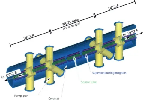
Pump port

Cryostat

Figure 2-2: The Windowless Gaseous Tritium Source (WGTS) and Pumping Sections. Printed from [6].

trons before the main spectrometer, a background due to ionization of residual gas in the main spectrometer is reduced. The remaining high-energy electrons then pass through a 2m transport system of two superconducting solenoids and then into the main spectrometer. This spectrometer measures this last approximately 300eV of the beta spectrum with an energy resolution of 0.93eV. The rate of electrons entering into the main spectrometer will be approximately 103 _{per second.[9] The pre-spectrometer}

has an outer diameter of 1.7m and is 3.38m long. The main spectrometer has an outer diameter of 10m and a length of 23m. Both spectrometers are maintained at a pres-sure of less than 10- 11_{imbar. [6]}

The electrons that leave the main spectrometer will then travel through another short transport system and finally impinge upon a multi-pixel, ultra-high energy res-olution silicon semiconductor detector. In this way, the energy spectrum of the elec-trons created via beta decay in the WGTS can be examined by dialing the retarding voltage of the spectrometer. [6]

AI

2.4.2

The WGTS in Detail

As discussed, a very small fraction of the beta spectrum is relevant to the determina-tion of the neutrino mass, so a very high count rate of beta decays is needed to obtain the statistics necessary for experimental observation. This high decay rate is accom-plished in the WGTS, which yields a beta decay rate of approximately 1011 decays per second. The WGTS consists of a tube, 10m long and 90mm in diameter. Molecular tritium gas, T2, maintained at a high isotopic purity of greater than 95%, monitored

by Raman spectroscopy, is injected into the center of the WGTS through over 250 holes of 2mm diameter (to avoid gas jets) at a rate of 40g/day (with stability level 0.1%). From the injection point, the tritium travels the length of 5m via diffusion to either end of the tube, spending a time of ls in the WGTS. As a result, each single tritium molecule has a probability of about 10-' to decay within the WGTS. [6]

The tritium within the WGTS is maintained at a temperature of 27K with a stability to 0.1%. A low temperature is desirable because it decreases the random thermal motion of the tritium and allows this high density of tritium to be maintained at a relatively low pressure, and so, relatively low flow rate. This is important because it helps to reduce the Doppler broadening of the spectrometer measurements, which is the topic of this thesis. A temperature much lower than this, while it would fur-ther reduce this Doppler broadening, is not possible. This is due to the fact that, at lower temperatures, the tritium molecules may begin to cluster together. Since these clusters have different final electronic states than the molecular tritium, their for-mation would introduce new and uncontrollable statistical uncertainties. Therefore, the Doppler broadening at 27K represents the optimal balance between statistical uncertainties and cannot be removed by lowering the temperature further. [6]

The WGTS in encircled by superconducting solenoids that maintain the entire source at a magnetic field of 3.6T. This magnetic field serves to adiabatically guide the electrons produced in the source by beta decay to the ends of the WGTS. To maintain the high tritium concentration within the WGTS, the tritium is circulated within a nearly closed loop. This is accomplished by a differential pumping system of

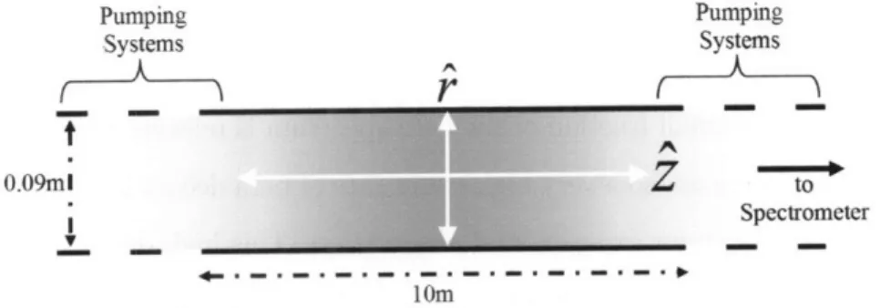
Pumping Pumping Systems Systems O.09mi V A to Spectrometer lOm

Figure 2-3: The WGTS coordinate system used in this thesis.

turbomolecular pumps located on either end of the WGTS. This differential pumping leads to a density/pressure profile within the WGTS that will be discussed in detail later. [6]

In our analysis, we will assume that the WGTS is axially symmetric, and thus, analysis of the system can be reduced to a two-dimensional analysis (we partially lift the one-dimensional assumption in Ref. [10]). Let us establish the coordinate system that z is the coordinate along the axis of the WGTS, and that the positive z direction points toward the main spectrometer. The other relevant coordinate is then r, the radial distance from the axis of the WGTS. Because of the rotational symmetry about the axis, we will consider only a two-dimensional plane described by r and z.

Chapter 3

Beta Decay

3.1

Fermi's Golden Rule

Fermi's Golden Rule is the rule that governs the transition rate of a system into a continuum of states. It can be derived, in quantum mechanics, from time-dependent perturbation theory, where the dependent Hamiltonian is expanded into a time-dependent and a time-intime-dependent portion:[5]

H(t) = Ho + H1(t) (3.1)

And Hi(t) is assumed to be expressible in the form

H'(t) = Hle-wt (3.2)

The final result is

RP-+ = -7 (fojH1Iji0) 2 _{6(Ef - E -_ ) (3.3)}

Ri-,f is the transition rate from state i to state f, and the superscripts denote to what order of the Hamiltonian the quantities correspond. This equation applies to many systems that undergo transitions, including nuclear decay. [5]

3.2

Tritium Beta Decay

Nuclear decays are governed by Fermi's Golden Rule (Eq. 3.3), where the "transi-tion" that occurs is the actual decay, where the parent nucleus decays into a daughter nucleus and possibly various other products. For nuclear decays, the golden rule sepa-rates into a matrix element and a phase-space factor. [1] The matrix element encodes the dynamical information about the decay, and the phase-space factor describes the kinematic information. Loosely speaking, the phase-space factor adds a weighting based on the relative number of different possible states and configurations available in a decay. One can think of the phase-space factor as characterizing the number of ways one can distribute the available energy of the decay among the momenta of the various products. The beta decay of the neutron has a relatively small amount of phase space available due to the relatively small difference between the rest energy of the parent and the sum of the rest energies of the products. This difference in rest energies, by relativistic energy conservation, is equal to the total kinetic energy available to the products in the decay, and is referred to as the decay's endpoint, (mentioned earlier) and is denoted by E0. Since the phase-space element describes the possible ways to distribute this kinetic energy between the particles (while con-serving momentum), the small size of this kinetic energy is a constraint that translates into a smaller phase-space factor. This is why the rest masses of the products have such a significant effect on the shape of the energy spectra in neutron beta decay; the rest-energies of the electron and perhaps the neutrino are non-negligible fractions of the total energy released in the decay. This is a reason why the low endpoint of tritium is so attractive in performing neutrino mass experiments that examine the shape of the beta spectrum. In decays with larger phase-space factors, one may be able to neglect the rest energies of certain products. [1] The beta decay of atomic tritium (3H, or T) is described by the equation:

So, for the specific case of atomic tritium decay, Fermi's Golden Rule takes the form:

[1]

d- = _ - CdpH± cd Pe (22r)4_6(pT

- - PHe+ - Pe)

2hmT (21r)32E,, (27)32EHie+

1

(21r)32EeJ

(3.5) Here, the subscript He+ denotes the 3He+ daughter. The matrix element can be

evaluated various ways. Ref. [1] expands the matrix element by using Feynman diagrams, while Ref. [11] performs a full relativistic treatment by expanding the matrix element in a sort of a Taylor series. The relativistic argument is that IM12 is a Lorentz invariant term, and so, can be expanded as a sum over Lorentz invariant quantities. The most general form, up to two powers of momenta is then[11]

M 2 = A - Bp - P- - CPHe+ Piniti al + ... (3.6)

In general, A, B, and C are arbitrary constants, but Ref [11] argues that, for the tritium decay, A = C = 0, and B

$

0. Thus, combining Eq. 3.5 and Eq. 3.6, the total weighting factor for a given set of four-momenta of the three products is simply the phase-space factor multiplied by the dot product of the four-momenta of the electron and the neutrino. This is relevant to the simulations performed for this thesis, because the simulation package that is used produces four-momenta of products weighted solely by the phase-space factor. In order to transform these results into products specifically of tritium beta decay, this extra dot-product weighting is added. Eq. 3.5 and Eq. 3.6 can further be manipulated algebraically, momenta can be integrated over, and a final Fermi correction (see next section) can be added to produce the final electron energy spectrum given in Eq. 2.1.[2, 1, 11]

3.3

The Fermi Function

The above considerations, however, do not take electromagnetic forces into account. The electron that is being ejected carries a negative charge, and, as a result of loosing this electron, the daughter nucleus has a net positive charge. Therefore, we expect

Coulombic forces between these two charged products to affect the kinematics de-scribed above. Since the force is attractive, the actual speed of the electron (and so, its energy) is smaller than that predicted purely by kinematics. Because the full derivation of the Fermi function is beyond the scope of this thesis, let us try to un-derstand the effect and its dependencies qualitatively. First, we expect this effect to depend upon the charge of the daughter nucleus, Z, because this will affect the overall strength of the Coulombic force. Second, electrons ejected with low energies move at slower speeds than electrons ejected with higher energies. Consequently, lower energy electrons spend more time close to the daughter nucleus (i.e. in regions of strongest Coulombic attraction) than higher energy electrons. Therefore, the effect of Coulom-bic interactions will be larger for low energy electrons, so we expect this CoulomCoulom-bic effect to also be a function of the electron energy. This energy-dependent Coulombic effect therefore changes the weighting of electron energies in our spectrum, and its distortion should be largest in the lower energy region. We can characterize this effect then by multiplying the energy spectrum by a correction factor, F(Z, E). This factor, F(Z, E) is known as the Fermi function, and is quite complicated. However, in the non-relativistic limit, it can be approximated as[2]

F(Z, E) = x (1 - e- (3.7)

Where

21rZa

x = (3.8)

Where a is the fine structure constant, E is the total energy of the electron, and / is the velocity of the electron divided by c. An improved version of this approximation is presented by Ref. [12]

F(Z, E) = x (1 - e-x)- 1 [ao + al/3] (3.9)

Here, the constants ao and a, are determined empirically to be ao = 1.002037 and a, = _{-0.001427. Eq. 3.9 agrees with the relativistic calculations of Ref. [13] over the}

energy range involved in the determination of the neutrino mass. Thus, this is the expression for the Fermi function that is used in the calculations in this thesis.

3.4 The Kurie Plot

The effect of the neutrino mass upon the beta spectrum is not very visibly apparent unless different spectra corresponding to different neutrino masses are superimposed. An alternative representation of the beta spectrum, called the Kurie plot, makes the effect of a non-zero neutrino mass quite vivid. When comparing different beta spectra, Kurie plots are often used, due to their relatively simple, mostly linear nature. [2]

The beta energy spectrum, Eq. 2.1, reduces to the following expression in the case of a zero neutrino mass:

d

2

_N

dtdE = KF(E, Z)p(Etot)(Eo - E)2 (3.10)

where Etot is the total energy of the electron (E + mec2). If we define N(E) to be the number of electrons with kinetic energy within a range of [E, E + dE] in a time interval dt, then we can rearrange Eq. 3.10 as follows

[

N(E)

No(E), 1/21/2= _{C(Eo - E)}

(3.11)

pEti t N(E Z)

Thus, if we plot the quantity EtoF(E,Z) against the electron energy, the plot will be linear (for the case of zero neutrino mass) and will intercept the E-axis at the endpoint energy, Eo0.[2, 9] However, due to the difference between Eq. 2.1 and Eq. 3.10, the Kurie plot for a beta spectrum corresponding to a non-zero neutrino mass will be mostly linear but will contain a slight dip near the endpoint. (See Fig. 3.4).

I Effect of m, on the Beta Spectrum of T2 i E

Electron Kinetic Energy (keV)

;07

Electron Kinetic Energy (keV)

Figure 3-1: Beta Decay Spectra and corresponding Kurie Plots for stationary (in the rest frame of the decay) T2 decay for m, = 1 and 0 eV/c2. Note that, for m, - 0,

the Kurie plot is a straight line, whereas the Kurie plot for m, = 1 eV/c2 dips near the endpoint. This figure is constructed from the same stationary decay data sets as in Figs. 6.2.1-6.2.1.

Effect of rm on the Kurie Plot I

3.5

Molecular Decay and Final State Distribution

The tritium source that will be producing the beta decays in the KATRIN experiment is tritium gas. This tritium gas consists primarily of tritium molecules, T2. This

molecular tritium gas is inherently more complicated than the pure, atomic tritium

considered in Eq. 2.1. Molecules can possess certain vibrational and rotational states that pure atoms do not. For instance, if we consider a classical toy model of a diatomic molecule, such as T2, we model the molecule as two hard spheres (the atoms) connected by a spring (the bond between the atoms). Let us consider the states of a molecule at rest in this model. One state consists of the two spheres remaining at rest with respect to one another, with the spring remaining at its rest length. This is analogous to the state of just one single sphere. However, the spheres may also oscillate towards and away from each other symmetrically about the center of the spring. This latter state has a higher energy associated with it than the former, however in both cases, the molecule is at rest, so this energy is not associated with the motion of the molecule's center of mass. Thus, this second state possess a certain

internal energy, due to the vibrations of the constituent atoms. A single hard sphere

does not possess such a vibrational state. Furthermore, rotations of the "molecule" about different axes now have different energies because the molecule is not spherically symmetric, as the atom is. Of course the true rotational and vibrational states of a molecule is much more complicated and is governed by quantum mechanics, but this model serves to lend an intuitive picture to the notion of vibrational and rotational states.[14, 15] The decay of molecular tritium (3

H2, or T2) is described by[6]

T2 (3HeT)+ + e- + Pe (3.12) Since the (3HeT)+ ion is a molecule, it can exist in a number of rotational-vibrational

states. Thus, when T2 decays, a certain amount of the energy released by the decay goes into exciting a rotational-vibrational state of the (3_{HeT)+ ion. We will} hence-forth refer to the state of the (3_{HeT)+ ion in Eq. 3.12 as the "final state." Energy} conservation then dictates that the total kinetic energy of the decay (the endpoint)

is decreased by an amount equal to this final state energy. Thus, the endpoint of the molecular tritium decay, Eq. 3.12, is actually a function of the final state of the

(3 HeT)+ molecular ion. The distribution of these final states therefore influences the

shape of the observed beta spectrum near the endpoint. Since the determination of the neutrino mass is dependent upon this very shape, simulations of the tritium de-cay in KATRIN must include this final state distribution in order to be accurate. In addition to the rotational-vibrational states mentioned above, the daughter (3HeT)+ could also exist in a number of electronic excited states, which would also affect this final state distribution. However, analysis has shown that these excited states are negligible compared to these rotational-vibrational states. [6] Therefore a distribu-tion of final states due to rotadistribu-tional-vibradistribu-tional states is sufficient for the purposes of KATRIN. The distribution of such states is, again, determined by Fermi's Golden Rule, Eq. 3.3. Here, the two wavefunctions considered are that of the parent T2 and

that of the daughter (3HeT)+. The H1 is an expression that includes the recoil of the emitted electron. From this starting point, simulations are performed under the sudden approximation to produce the final state distribution. The sudden approxi-mation is the assumption that the interaction between the electron and the (3_HeT)+

ion is negligible. [15] The distribution produced consists of a discrete, low-energy dis-tribution, and a high-energy tail. The tail is described by[14]

(

8e- 4_arc• _an(K)/ _{2 dE (313)} P(E) 14.7 1-e47r (1 + 2)2 eV(3.13)

where the probability P(E) is given as a percent, and r = (E - 45eV)/13.606eV.

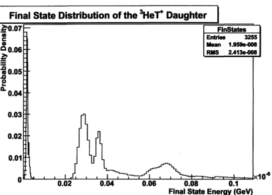
For the purposes of my simulation, I discretized the tail in intervals of 0.1eV, to match the smallest resolution given for the discrete portion, and combined both together into a histogram (Fig. 3.5). The final state energies thrown from this histogram were added to the rest mass of the (3_HeT)+.

U.UL U.Uq U.UU U.UO U. 1

Final State Energy (GeV)

Figure 3-2: The distribution of final states of the (3HeT)+, constructed from Eq. 3.13 and the data given in 3.12.

Chapter 4

Thermal Motion and Doppler

Shifts

The equation describing the beta spectrum of tritium decay, Eq. 2.1, is valid in the rest frame of the parent tritium. When the parent tritium is moving, it possesses more energy due to its kinetic energy, so the products of the decay must also have more energy in total. As discussed in Chapter 2, the tritium in the WGTS is moving for two reasons: random thermal motion, and the velocity profile due to pumping. Here we will consider the former. Because the source molecules are at a finite temper-ature, they possess a finite amount of thermal energy in the form of random motion. This random distribution of initial velocities translates into random shifts in the en-ergy of the decay products, and so, tends to smear out the observed beta spectrum. This phenomenon is known as "Doppler broadening" of the spectrum. The name comes from the fact that, spectrometry is often performed to measure the spectrum of light, and so, the velocity of the light source causes a frequency shift (Doppler shift) in the frequency of the observed light. Even though the term "Doppler shift," strictly speaking, correspond to frequency shifts, the terminology is also used to de-scribe spectrometry experiments in general; even those that measure energy spectra of particles, like KATRIN.

Therefore, because the initial velocity of the tritium gas molecule affects the en-ergy of the emitted electron, a simulation of the electron enen-ergy spectrum requires a

probability distribution for the initial velocities of the T2 molecules. To this end, we

can use the famous Maxwell velocity distribution. Because the T2 gas in the WGTS

consists of diatomic molecules, let us consider the significantly general treatment of the Maxwell velocity distribution performed in Ref. [16]. This treatment considers the effects of the internal energy states (see Chapter 3) of the T2 molecule.

Even though the gas in the WGTS is of very high purity, this purity is not 100%. Therefore let us consider a general dilute gas, which consists of a mixture of different types of molecules. Let us then consider a polyatomic molecule of mass m (a T2

molecule in our case) within this gas, with center of mass position and momentum r' and 'respectively. If this gas is sufficiently dilute such that it can be treated as ideal, then we may neglect intermolecular interactions. If we also neglect external forces, such as gravity, the energy of our particle is given by

E -2m+ Eint

_2m

(4.1)

where Eint represents the internal energy due to the rotational-vibrational state of the molecule. This internal state must be treated quantum mechanically, and is indepen-dent of position, due to the neglect of intermolecular interactions. However, due to the diluteness of the gas, the translational component of the molecule's state can be approximated to be classical, and the particle itself can be treated as a distinguishable particle.

The gas in the WGTS is maintained at a constant temperature, so the molecule is in contact with a heat reservoir, and therefore follows the canonical distribution. The canonical distribution states that a particle in contact with a heat reservoir of temperature T, has a probability to be in a state, a of

P, oc e- 0E. (4.2)

where 3 = ~ kb is Boltzmann's constant, and E, is the energy of state a. Applied to the T2 molecule in the gas, this means that the probability of the molecule being in

space volume d3' centered about 7, and being in an internal quantum state denoted

by the quantum number s is given by

PS (_,p- oP e- e-OEjnt(s)dj 3d3- (4.3)

2m e (43

In theory, the internal states of the T2 molecule before it decays should affect the beta spectrum to some degree. However, the value of the rest mass of T2 that is currently used in KATRIN analysis is simply twice the rest mass of atomic tritium, T.[17, 18, 10] This is only approximately correct as it neglects the binding energy of

T2, which is estimated to be negligible compared to uncertainties in other quantities used in the calculations. [18] Therefore, the effects of the initial internal states of T2

would be beyond the precision of the rest energy of T2, and so the inclusion of these effects at this stage would be artificial and require a more detailed knowledge of

T2. Therefore, in the simulations in this thesis, the initial internal states of T2 are neglected.

Therefore, to get the probability for a certain position and momentum range only, we sum over all states s in Eq. 4.3. The result is simply an overall constant which is irrelevant, for the final probability density will be normalized. We may also integrate over F since we are interested in obtaining the velocity distribution, which is a function of = - only. The result is simply the product of three identical Gaussian

distributions, one for each component of the velocity. Normalization results in the Maxwell velocity distribution: the probability for a molecule to have a velocity in a range d3J about a value of I is[16]

(

3/2

m 2

-fmv(U)dd 3 2kT) e 2d3V (4.4)

27rkbT

If we are only interested in the speed of the particle, then we can change from Carte-sian to spherical coordinates (d3& = v2 _{sin OdvdOdq) and integrate over all directions}

(over 0 and q) to obtain the Maxwell speed distribution[16]

(M

3/2 m2 2

fms(v)dv = (2kbT) 41rv e 2kbT dv (4.5)

Which gives the probability for the particle to have a speed between v and v + dv. These are the velocity distributions used in this thesis to determine the random thermal velocities. This will also be used in the next chapter in the analysis of the fluid velocity profile. Note that we are able to use these standard forms of the Maxwell distributions because we neglected the initial states and the effect of gravity. To correct for gravity, one could include a term of the form e-Omgz, where g is the

acceleration due to gravity. However, this is unnecessary, because the change in gravitational potential over the diameter of 0.09m is negligible and inclusion of this factor would just add fruitless computation time to the simulation. Also, if one were to include the initial states of T2, one would have to return to Eq. 4.3, or include an