HAL Id: hal-00399698
https://hal.archives-ouvertes.fr/hal-00399698
Submitted on 28 Jun 2009
HAL is a multi-disciplinary open access
archive for the deposit and dissemination of
sci-entific research documents, whether they are
pub-lished or not. The documents may come from
teaching and research institutions in France or
abroad, or from public or private research centers.
L’archive ouverte pluridisciplinaire HAL, est
destinée au dépôt et à la diffusion de documents
scientifiques de niveau recherche, publiés ou non,
émanant des établissements d’enseignement et de
recherche français ou étrangers, des laboratoires
publics ou privés.
in satellite imagery
Amandine Robin, Lionel Moisan, Sylvie Le Hégarat-Mascle
To cite this version:
Amandine Robin, Lionel Moisan, Sylvie Le Hégarat-Mascle.
An a-contrario approach for
sub-pixel change detection in satellite imagery.
IEEE Transactions on Pattern Analysis and
Ma-chine Intelligence, Institute of Electrical and Electronics Engineers, 2010, 32 (11), pp. 1977-1993.
�10.1109/TPAMI.2010.37�. �hal-00399698�
An a-contrario approach for sub-pixel change
detection in satellite imagery
Amandine Robin, Lionel Moisan, and Sylvie Le H´egarat-Mascle
Abstract—This paper presents a new method for unsupervised
sub-pixel change detection using image series. The method is based on the definition of a probabilistic criterion capable of assessing the level of coherence of an image series relatively to a reference classification with a finer resolution. In opposition to approaches based on an a priori model of the data, the model developed here is based on the rejection of a non-structured model — called a-contrario model — by the observation of structured data. This coherence measure is the core of a stochastic algorithm which selects automatically the image subdomain representing the most likely changes. A theoretical analysis of this model is led to predict its performances, in particular regarding the contrast level of the image as well as the number of change pixels in the image. Numerical simulations are also presented, that confirm the high robustness of the method and its capacity to detect changes impacting more than 25% of a considered pixel under average conditions. An application to land-cover change detection is then provided using time series of satellite images.
Index Terms—change detection, a-contrario modeling,
signifi-cance test, sub-pixel, mixture model, image series
I. INTRODUCTION
T
HE detection of change areas using an image series is an important issue in image processing due to the large number of impacted applications, including in particular remote sensing [1]–[3], medical diagnosis [4], [5] and video surveillance [6], [7]. Even though more and more sensors are specialized in order to provide fine information dedicated to a specific range of applications, the intrinsic sensors charac-teristics generally result in a trade off between fine spatial resolution and fine spectral resolution or high time frequency. Therefore when a fine spectrum or a high time frequency is required to discriminate the target of interest (and prefered to a fine spatial resolution), this latter may be smaller than the pixel size. In such cases, providing efficient solutions for sub-pixel change detection is of crucial interest.This work has been initially motivated by the detection of land cover changes using remote sensed images. In this context and in particular for emergency applications such as floods or fires, the use of data acquired with a high time frequency is mandatory but the changes of interest may impact only a fraction of the observed pixel. Apart from emergency
A. Robin is now with the department of Computational and Applied Mathematics, University of the Witwatersrand, Johannesburg, South Africa. The main part of this research has been done when she was with the Laboratory of Applied Mathematics (MAP5), University of Paris Descartes e-mail:[email protected].
L. Moisan is with the Laboratory of Applied Mathematics (MAP5), University of Paris Descartes, Paris, France e-mail: [email protected].
S. Le H´egarat-Mascle is with the Fundamental Electronic Institute (IEF), University Paris Sud XI, 91405 Orsay, France e-mail:[email protected].
applications, changes can typically consist in natural land-cover transformations (intra or inter-annual variability) or human-induced changes (e.g. forest cuts, crop rotation). The approach presented here applies as well to multitemporal change detection using image time series as to bi-date change detection using single or multi-spectral images.
In the literature, a wide range of change detection methods has been proposed to analyze image series (with all images to the same spatial resolution). Most of them are based either on classification processes (post-classification comparison, joint classification [8] or fusion of classifications [9]), on change vector analysis and thresholding [10]–[12], or on predictive models [13], [14]. Some methods use Markov Random Fields in order to take into account the spatial neighborhood in the difference image [15], [16] and, more recently, a Hopfield-type neural network was proposed to model spatial correla-tions [17]. For more details, good overviews are given by [18], [19]. All these methods generally lead to limited results due to misregistration errors or illumination variations, which introduce some alterations of the signal that should not be detected as true changes (e.g. camera motion, sensor noise, shadows, atmospheric absorption, etc.). Even if pre-processing (e.g. geometric or radiometric corrections) are generally per-formed in order to avoid such limiting factors, they are only partly weakened and hence need to be taken into account. Moreover, some typical issues such as the definition of an a priori model or the choice of a detection threshold remain. In addition, very few works focused directly on the sub-pixel change detection problem. An early reference is [20], restricted to edge detection using zero-crossings of the Laplacian. More recently, [21] provided a supervised method restricted to change detection in pairs of images, [22] used an unmixing model for target detection in hyperspectral images and [23] estimated alternately class means and proportions in order to determine changes by comparing a CR time series to a HR classification.
Here, given the methodological concerns previously pointed out, we propose a novel, efficient and fully unsupervised approach to perform sub-pixel change detection by comparing a coarse resolution (CR) time series to a former high resolution (HR) reference classification. Such a comparison let us follow objects which are observable in the HR classification but often impossible to distinguish at a coarse resolution, meanwhile avoiding the frequent inter-calibration problems encountered in the literature. Compared to existing methods, this choice also highly improves robustness in terms of noise and lightning conditions, as the comparison refers to a minimal description of the initial state. Moreover, taking a classification
for reference rather than an image or an image series enables us to reduce prior hypotheses on the expected evolution.
The theoretical framework of the approach we propose is the so-called a-contrario detection, that was first proposed in [24] for the detection of alignments in images, and then developped for various tasks such as the analysis of histogram modes [25], the recovery of stereo point matches [26], motion detec-tion [27], the detecdetec-tion of spots in textured background [28], etc. The main principle driving a-contrario detection is a perception principle due to Helmholtz, first formulated in the context of image analysis by Lowe [29]. It basically says that we perceive a structure in a set of objects (say, an alignment in a set of black dots drawn on a white sheet of paper) when their configuration is too unlikely to happen by chance. This principle is formalized in the a-contrario framework using two ingredients: first, a naive (non-stuctured) model, which describe the random distribution we expect in case no structure is present (the classical H0 hypothesis in statistical decision
theory); second, one or several measurements related to the stucture we want to detect. With these two ingredients, the a-contrario framework allows to combine all measurements into a single real-valued function (called NFA, for Number of False Alarms), that can be thresholded to select saliant structures. Compared to the classical statistical decision theory, the a-contrario framework has several advantages:
1) No H1 hypothesis has to be formulated, which make
a-contrario models easier to build and less sensitive to questionable modeling choices;
2) The NFA function is easy to compute, because it does not aim at the control of the probability of a false alarm (which is often impossible to compute in the case of non-independent tests), but at the control of the expectation of the number of false alarms, whose computation can be performed by considering each test independently; 3) It guarantees that the number of (wrongly) detected
structures under H0 by threshloding the NFA function
to ε is, in average, less than ε.
The last property is responsible for the name “NFA”, which can be defined in a general setting [28]:
Definition 1.1 (Number of false alarms): Let (Xi)1≤i≤N
be a set of random variables. A function F (i, x) is a NFA (Number of False Alarms) for the random variables (Xi)if
∀ε > 0, E [|{i, F (i, Xi)≤ ε}|] ≤ ε. (1)
Assume that the Xi random variables represent the
measure-ments that characterize the structures we want to detect (that is, the measurement xi of Xi will be all the higher than the
i-th structure is saliant). Then, according to [28] (Proposition 2 p. 318), the function N F A(i, xi) = ni· P(Xi≥ xi) (2) is a NFA as soon as X i 1 ni ≤ 1 (3) (and in particular if ni= N for all i).
One important property of the a-contrario framework is that it reduces all detection parameters to one unique parameter:
the expectation of the number of false alarms ε. This is a key point dealing with unsupervised detection as, in practice, fixing the number of false alarms (e.g. to 1) makes the detection fully automatic. Moreover, this criterion used jointly with a random sampling algorithm leads to a very robust change detection method, in particular with regard to the proportion of change pixels in the image (which is a common limiting factor in the literature).
This paper is organized as follows. Section II describes the residual error on which the change detection is based. Section III details the a-contrario detection model. Section IV provides a theoretical analysis of the model performances when the main image parameters vary. In Section V, we propose an algorithm based on a random sampling strategy, in order to provide a robust estimation without considering all image subdomains. Section VI presents particular issues occuring in the multitemporal case and the solution adopted. Section VII provides experimental results and illustrates the performance of the approach in the case of land-cover change detection using remote sensing data. We end with concluding remarks in Section VIII.
II. RESIDUAL ERROR
The first step in building a change detection method is to define a relevant error measure regarding the application. Here, we assume that a HR label map is available and describes the reference state. The label map is considered as an application that assigns a label l ∈ L to each pixel of the HR image domain DHR. We aim at localizing the changes as areas where
the HR label map no longer corresponds to the CR image time series. Hence, the HR label map acts like a mask through which the spatial coherence of the image time series can be studied, and the detected changes will consist in parts of the time series that are not coherent with the reference label map. Such formulation a priori enables the detection of sub-pixel changes. Moreover, using a classification as a reference rather than an image time series is interesting as it puts a weaker prior on the expected evolution. It also enables to overcome typical intercalibration problems between dates. In Section VIII, we also show how a radiometric image, after quantization, can be considered as a reference in an application to video surveillance.
Denote DCRthe CR image domain, T the set of acquisition
dates and assume that all images of the time series are well co-registered. The observed CR time series is denoted v = (v1,· · · , v|T |) where for each date t ∈ T , the grey-level
image vt is a real-valued function defined on DCR. In order
to establish the link between the HR label map and the CR time series, let us assume that each CR image corresponds to the block average of a HR image of the same scene. Let N = |DHR|/|DCR| be the number of HR pixels that
are contained in a CR pixel and, for any pixel y ∈ DCR,
Nl(y) be the number of HR pixels with label l represented
within pixel y. The proportion of label l within pixel y is then αl(y) = Nl(y)/N and by definition, Pl∈Lαl(y) = 1. For
sake of simplicity, the model will be from now on considered in the monotemporal case, and the multitemporal case will be
discussed in section VI. If µ = (µ(l))l∈L stands for the mean
intensity characterizing labels l, then the intensity of a pixel y∈ DCR is estimated by
ˆ
v(y, µ) =X
l∈L
αl(y)µ(l). (4)
Practically, this block-average hypothesis may be only roughly satisfied. In general, CR values are obtained by a modulation transfer function which is not an indicator function as sup-posed by the block-average hypothesis. However, Equation 4 boils down to the linear mixture model [30] which is com-monly used in the remote sensing community since numbers of applications showed its relevance even when the hypothesis of block-average is not valid (see [31], [32]).
Then, knowing the label proportions, an optimal HR re-construction ˆvD may be obtained by using the label map and
choosing label means (µ(l))l∈Lthat minimize the
reconstruc-tion error, equal to δ(vD) = r min µ∈RL||vD− ˆvD|| 2 2, (5)
where vDis the CR time series restricted to the subdomain D
of DCR.
At this stage, the main detection issue is the definition of an a priori threshold on the residual error δD, in order to
decide between changes and no-changes. This threshold should be an appropriate combination of the residual error δD and
the size of the subdomain D. Indeed, even without changes, larger subdomains are expected to yield larger residual errors since they involve more pixels. The method we present here estimates jointly the label means and the change pixels using a random sampling strategy (see [33]), thus ensuring a high robustness to the amount of change pixels or outliers in the image.
In section III, we build an a-contrario detection model that enables to combine these parameters into a single proba-bilistic criterion allowing the detection of the most coherent subdomain with a given classification (namely a given high-resolution label map) meanwhile controlling the expected number of false alarms. The complementary of this subdomain is then considered as the set of pixels presenting some changes.
III. A-CONTRARIO CHANGE DETECTION MODEL
A. Definition of a coherence measure
In the framework of a-contrario modeling, the idea is to detect an image subdomain as a large deviation from a naive model. To that aim, we introduce a measurement of the coherence between the HR label map describing the state of reference at a given date t0 and the observed CR image at
date t based on the degree of contradiction which it implies refering to a non-structured model (the naive model).
Definition 3.1 (A-contrario (naive) model for CR): The a-contrario model (H0(m)) for the CR image is a random
Gaussian vector V ∼ N (m, σ2I
|DCR|), where m ∈ R
|DCR|and
σ > 0are fixed, and I|DCR|is the identity matrix in dimension
|DCR|.
The choice of the parameters of the naive model is discussed in Section III-B.
Following Helmholtz principle, we focus on image sub-domains for which the quadratic error measured between the image and its estimation is too small to be reasonnably explained by randomness. Actually, we consider the level of surprise of observing an intensity map vD on a subdomain D
of DCR which, for a given choice of µ, is particularly close
to the intensity estimated from µ and label proportions within pixels. A detection threshold δDon the error δ(VD)could then
be chosen such as ensuring that
P(∃D, δ(VD)≤ δD)≤ ε, (6) where ε is a fixed parameter (e.g. 10−3) and δ(V
D) is the
quadratic error obtained considering the random field V de-scribed by the a-contrario model (Gaussian white noise image). The parameter ε enables us to supervise the test reliability. Indeed, the smaller ε is, the more demanding and reliable the test. Now, dependences between the random variables (δ(VD))D∈DCR are very difficult to estimate, which makes the
explicit calculation of P(∃D, δ(VD)≤ δD)impossible.
Following the framework introduced in [24], we suggest to measure the expectation of the number of false detections rather than controlling the probability of having at least one false detection. This measure is defined in order to guarantee a number of false detections on random data as low as desired, using a quantization of the number of tested subdomains (through a weighting coefficient called “number of tests”).
Proposition 3.1 (Number of Falses Alarms): Consider a function η : N → (0, +∞) and, for any subdomain D ⊂ DCR,
the quantity
N F A(D, δ(vD), σ, m) = η(|D|) · PH0[δ(VD)≤ δ(vD)], (7)
where PH0[δ(VD) ≤ δ(vD)] stands for the probability of
observing a minimal error δ(VD) less than δ(vD) under
Hypothesis H0(m). Then, the NF A function is a number of
falses alarms provided that X
D∈DCR
1
η(|D|) ≤ 1. (8) For any ε > 0, we shall say that a subdomain D of DCR is
ε-meaningful if NF A(D, δ(vD), σ, m)≤ ε.
Proof — Let us set N = 2|DCR| and define, for i ∈ {1, ..N},
Xi = −δ(VDi), where (Di)1≤i≤N represents all subsets of
DCR. Taking ni = η(|Di|), we then have
N F A(Di, δ(vDi), σ, m) = N F A(i, xi)
(the right term being defined in Equation (2)), hence we know thanks to [28] (Proposition 2 p. 318) that (7) defines a Number of False Alarms as soon as Equation (3) — or equivalently, Equation (8) — holds. ¤ Choosing a function η that satisfies (8) is then sufficient to guarantee a number of false alarms less than ε. In this study, the first natural choice for the η function is a uniform weight on all subdomains of DCR, i.e. η(|D|) = |{D, D ⊂ DCR}| =
2|DCR|. This choice ensures less than ε false detections (on
the average) as PD⊂DCR 1
2|DCR| = 1. It distributes the risk
and even if they overlap) as, for all subdomain D ∈ DCR, the
probability of mistakenly detecting D is
PH
0(δ(VD)≤ δ(vD)) =
ε
2|DCR|, (9)
where the right term does not depend on D. With such a choice, a subdomain with medium size is more likely to be detected by chance, as such subdomains are more numerous. Now, notice that choosing η is an opportunity to introduce some a priori for the detection. In practice, changes generally affect a minor part of the image (≤ 50%) but in order to maintain the genericity of the method, we suggest an alternate function η that equally considers subdomains with any given size.
More precisely, we suggest to distribute the risk uniformly with respect to the subdomain size, by taking for any D ⊂ DCR, η(|D|) = |DCR| µ |DCR| |D| ¶ . (10)
This is a valid choice for the weight function η, since it satisfies Equation (8) : X D∈DCR 1 η(|D|) = X D∈DCR 1 |DCR|¡|D|D|CR| ¢ = |DCR| X k=1 X |D|=k 1 |DCR|¡|D|D|CR| ¢ = |DCR| X k=1 µ |DCR| k ¶ 1 |DCR|¡|DkCR| ¢ = |DCR| 1 |DCR| = 1.
In the following sections, this choice of η will be considered and we will set ε = 1 in order to ensure less than one false detection on average while making the method fully automatic. Using the a-contrario hypothesis given by Definition 3.1, the NF A can be computed explicitly.
Theorem 3.1: Using the a-contrario hypothesis denoted by H0(m), for all m ∈ R|DCR|, the number of false alarms
associated to a subdomain D of an image v is determined by
N F A(D, δ(vD), σ, m) = η(|D|) · f(q, δ(vD), σ, m), (11)
where η(|D|) = |DCR|¡|D|D|CR|
¢
, q = |D| − |L| (|L| being the number of labels) and, for all q ∈ N+
f (q, δ, σ, m) = 1 σq(2π)q2 Z Bq(δ) e−12 Pq i=1( xi−mi σ ) 2 dx1...dxq,
Bq(δ)being the ball of Rq with center 0 and radius δ.
Proof — The proof is detailed in Appendix A, it is a conse-quence of Proposition 3.1 and the explicit computation of the NFA function for the chosen hypotheses. ¤
B. Discussion on the parameters
The naive model H0 (see begining of Section III) used for
the definition of this criterion depends on two parameters: the mean m and the variance σ2. In this section, the choice
of these parameters is discussed. It is mainly guided by the condition of no detection in a noise image (i.e. following the naive model) but also by the fact that the NF A needs to be minimized.
First, we consider the naive model according to which the mean CR image is a constant image.
Hypothesis Ha
0: The mean vector m of the naive model
H0(m)is (θ, θ, · · · , θ)T (for a given θ ∈ R) and the standard
deviation σ is a priori fixed.
Corollary 3.1: Under hypothesis Ha
0, the number of false
alarms is N F Aa(D, δ(vD), σ) =|DCR| µ |DCR| |D| ¶ · f(q, δ(vD), σ, 0), (12) with q = |D| − |L|.
Proof — Let AD = (αl(y))y∈D,l∈L be the matrix of label
proportions restricted to the subdomain D. The proof comes from Theorem 3.1, remarking that as the sum per line of ADis
1, the vector space R(1, 1, · · · , 1)T is included in the image
space of AD, denoted ImAD. In particular, since the mean
vector m belongs to this set, it satisfies ADm = m. Hence, if
the matrix P denotes the orthogonal projection onto the space (ImAD)⊥, the mean vector projected by P boils down to the
null vector (P m = 0) and PHa
0[δ(VD)≤ δ(vD)] = f (|D| − |L|, δ(vD), σ, 0)
thanks to (27) (see Appendix A, proof of Theorem 3.1). ¤ An alternate hypothesis for the parameters of the H0model
is to assume any mean CR image and a fixed variance for each pixel.
Hypothesis Hb
0: The mean vector m of the naive model
H0(m) is any unknown vector of R|DCR| and the
standard-deviation σ is a priori fixed.
As m is an unknown parameter of the NF A model, we are looking for the model which best enables to control the number of false alarms for all H0(m) models, where m ∈
R|D|. Hence, we need to consider the most pessimistic NFA given by
arg max
m∈R|D|N F A(D, δ(vD), σ, m).
This maximum happens to be reached when the mean of the H0 model is null, which leads to the following result.
Proposition 3.2: Under Ha 0 or H0b hypotheses, N F A(|D|, δ(vD), σ) =|DCR| µ |DCR| |D| ¶ ¯ f (q, δ(vD), σ), (13) where, ¯ f (q, δ, σ) ≡ f(q, δ, σ, 0) = 1 σq(2π)q2 Z x1,q∈Bq(δ) e−12 Pq i=1( xi σ) 2 dx1...dxq, and q = |D| − |L|.
Proof — The proof relies on the Lemma B.1 (see appendix B) as its application to f implies directly
N F Ab(|D|, δ(vD), σ) = max m |DCR| µ |DCR| |D| ¶ · f(|D| − |L|, δ(vD), σ, m) = |DCR| µ |DCR| |D| ¶ · f(|D| − |L|, δ(vD), σ, 0) = N F Aa(|D|, δ(vD), σ). (14) Hypotheses Ha
0 and H0b lead to the same number of false
alarms, denoted NF A, which proves Proposition 3.2. ¤ According to this result, the naive model H0(0) is the most
contrary model in the family of models H0(m), where m ∈
R|DCR|. Then, considering the mean vector m = 0, rejecting
H0(0)implies the reject of all the naive models of the family
H0(m)and it enables to free from the mean parameter.
Finally, note that numerically speaking the number of false alarms is easier to compute from the following form.
Corollary 3.2: Under Ha 0 or H0b hypotheses, N F A(|D|, δ(vD), σ) =|DCR| µ |DCR| |D| ¶ Γinc µ q 2, δ(vD)2 2σ2 ¶ , (15) where q = |D| − |L| and, for all x ≥ 0 and a > 0,
Γinc(a, x) = 1 Γ(a) Z x 0 e−tta−1dt.
The obtained criterion hence depends only on the size of the subdomain, on the error which is computed on this subdomain and on the standard deviation of the naive model H0. As these
first two parameters are directly determined from the studied images for a given sub-domain, the standard deviation of the naive model σ is the only parameter to set a priori. Here, we suggest to set it to the empirical variance of the observed image. Such choice is motivated by the fact that it ensures the absence of any detection in a white noise image on average.
C. Comparison with Multiple testing procedures
The calculation of the number of false alarms is related to the statistical problem of multiple testing [34] as it takes the number of performed tests into account in its definition. Multiple testing procedures have been developped in order to process large amounts of data without increasing the av-erage number of erroneous detections. A classical statistical approach for testing N random variables while controlling the number of false alarms (also called false positives) would be to threshold the N p-values individually to a level α, thus ensuring an average number of false positives less than αN, i.e. non-decreasing according to the number of tests. Assuming that the N tests are independent, the probability of occurence of one error of the first order is then 1 − (1 − α)N, which is
e.g. 40% for 10 tests with a level 5%.
As far as the change detection issue is concerned, it could be considered as an adequacy test, assuming a theoretical model for the CR image. For instance, a model such as those where the random variables corresponding to each pixel are assumed to be Gaussian, with parameters related to the occupation
rate of each class represented within the pixel and to class characteristics, can be considered as an a priori model. The 2|DCR|tests of all subdomains of DCRare then considered with
the following hypotheses:
• H0(D): “the CR image restricted to the subdomain D is
not structured according to the reference classification.”
• H1(D): “the CR image restricted to the subdomain D is
structured according to the reference classification.” Hence, pixels that are detected as changes are those which satisfy the null hypothesis H0(D). This test can be performed,
for instance, with a χ2statistic [35]. Using previous notations,
the decision rule consists in rejecting H0(D) when δ(VD)≤
δ(vD). If each test of H0(D) against H1(D) is to the level
αD, then by definition the thresholds δ(vD) ensure that the
probability of mistakenly rejecting H0(D)satisfies
P(δ(VD)≤ δ(vD)| H0(D))≤ αD. (16) After performing N tests of hypothesis H0=∪D⊂DCRH0(D)
against H1 = H0c (so as to consider all sub-domains D), it
seems natural to reject H0 for H1 if there exist a subdomain
D∈ DCRsuch as the hypothesis H0(D)is rejected for H1(D),
i.e. such as δ(VD)≤ δ(vD). Let us remark that the probability
of mistakenly rejecting H0 then satisfies
P(∃D ∈ DCR; δ(VD)≤ δ(vD)| H0) ≤ X D∈DCR P(δ(VD)≤ δ(vD)| H0D) ≤ X D∈DCR αD. (17)
The naive approach previously mentionned would be to con-sider that each test is performed to the level αD = α,
independently from the tested subdomain and, consequently, that the probability of mistakenly rejecting H0is less than Nα
(e.g. 210 000
× 0.05 for a 100 × 100 image and a significance level α = 0.05). To avoid such an increase of first type errors, the Bonferroni procedure [36] aims at maintaining the probability of false alarms less than α > 0 while testing, for instance, all subdomains to a level αD≤ Nα. the H0hypothesis
is then rejected if αD≤Nα for all D ∈ DCR. This strategy is
very restrictive as each individual test is then maintained to a demanding threshold so as to control the rate of false alarms, even though errors of type 2 then increase. Hence, some detections tend to be missed by such procedure. Formally, the calculation of the number of false alarms (defined for N = 2|DCR| tests) is equivalent to Bonferroni procedure as it
simply boils down to test if NαD≤ α. However, their concept
is different and, in particular, the NF A enables to directly control the number of false alarms (false positives). Indeed, in opposition to Bonferroni procedure, it has an intrinsic meaning allowing, for instance, to decide the acceptation of exactly 10 errors out of 1 million tests on average (while a “test of level 10” has no meaning). The NF A definition that we use in practice is a variant of this procedure as the number of tests (N = |DCR|¡|D|D|CR|
¢
) considered for the NF A penalizes the tested subdomain according to their size, favouring those with large and with small size. Formally, it means testing all subdomains D with the level αD such as αD ≤ α
This choice enables to ensure an error of type 1 less than α as X D∈DCR αD≤ X D∈DCR α |DCR|¡|D|D|CR| ¢ ≤ α. (18) Numerous procedures have been proposed in the literature as alternatives to Bonferroni procedure [37], [38]. They are based on controlling the different error types such as, for in-stance, the FWER (Family Wise Error Rate) which controls the probability of obtaining at least one false positive, the PCER (Per Comparision Error Rate) which controls the expectation of the proportion of false positives among all tests or the FDR (False Discovery Rate) to control the expected proportion of mistakenly rejected hypotheses. In particular, the widely used Benjamini-Hochberg procedure [38] enables to controlling the FDR meanwhile considering all tests. Then, decision is taken by considering a significant test set instead of using each test individually. More precisely, as a first step, this procedure consist of sorting the p-values
p(1)≤ · · · ≤ p(i)≤ · · · ≤ p(N )
then, if k = max{i : p(i) ≤ Ni α} exists, of rejecting
H0(i) for i = 1 . . . k and thus ensuring a false discovery
rate F DR ≤ α. This procedure is less conservative than Bonferroni’s as it accepts all subdomains which p-values are less than pk whereas Bonferroni correction does not allow
the acceptation of subdomains which p-value is less than the threshold α/N. Finally, the Benjamini-Hochberg procedure globally detects a set of subdomains that do not contain any change meanwhile accepting some percentage of errors, but no subdomain is detected individually. In our context, considering the union of significant subdomains seems difficult as the detection of a collection of significant subdomains is hard to interpret. Hence, such procedure does not really seem to fit the considered problem. Moreover, the NFA values correspond typically to very weak probabilities (about 10−1000). Hence,
a threshold such as α/N on the NFA value would not be restrictive.
The relevance of the NFA definition relies on the fact that the expected number of false alarms of ε-meaningful events is less than ε. This property enables to automatically set the decision thresholds in order to ensure an a priori fixed number of false alarms (e.g. ε = 1). Generally, the most meaningful domain is retained, that is the one which minimizes the NFA (as the most coherent subdomain with the label map).
IV. THEORETICAL PERFORMANCES
A. Image model
The simple image model described here is used in order to consider separately the main detection parameters and, then, to study the sensitivity of the theoretical model according to each parameter. As a first step, let us consider an image u of the same size and resolution than the label map. Assume that any image u can be written as u = I + b, where I is a piecewise constant image and b a Gaussian noise image. Given a label map with |L| labels, the image I is assumed to be perfectly superimposable to the label map, with the corresponding label characteristic value mapped to each pixel (i.e. typically, a mean
label value image). The empiric image variance σ2 of u can
then be obtained directly from σ2 = σ2
I + σb2. Moreover, the
estimation of the label characteristics familly µ is assumed to be accurate in order to analyse the sensitivity of the number of false alarms. The quadratic residual error measured on average for each pixel is then σ2
b, which implies an average cumulative
quadratic error on a subdomain D of E£δ2
D¤ = |D| × σ 2 b.
Let us consider that the mean square error obtained on a subdomain of size |D| is δ2
|D| = |D| σ2b. Refering to
Equation (15), the number of false alarms associated to a subdomain of cardinal |D| which is part of a domain of cardinal |DCR| can be written as
N F A(|D|, δ|D|, σ) = |DCR| µ |DCR| |D| ¶ Γinc à |D| − |L| 2 , |D| 2((σI σb) 2+ 1) ! . (19)
This expression highlights the fact that the number of false alarms mainly depends on the following parameters : the considered subdomain size, the number of labels represented in the label map and the variances ratio σI/σb. As this ratio
can be interpreted as an image contrast measure, let us denote the image contrast by c = σI
σb (with c ≥ 0) and introduce
the parameter γ = 1
c2+1, γ ∈ (0, 1]. Moreover, the considered
subdomain cardinal can be expressed as a proportion p ∈ [0, 1] of the whole domain cardinal: p = |D|/|DCR|. The number
of false alarms of an image with contrast c, associated to a subdomain concerning a proportion p of the image, can then be expressed as F(p, |DCR|, γ) = |DCR| µ |DCR| p|DCR| ¶ Γinc µ p|DCR| − |L| 2 , γ p|DCR| 2 ¶ (20) for p ∈ ( |L| |DCR|, 1]and γ = 1
c2+1 ∈ (0, 1]. This new expression
is used for the performance and sensitivity analysis which is developped in the three next sections.
B. Sensitivity to the contrast level
In general, image comparison is improved when images have the same dynamic. As satellite image intensity values vary a lot with luminance conditions, the robustness to the contrast level is an important criterion for a change detection method relevancy.
First, let us focus on the particular case of an image with a null contrast (c = 0, i.e. σI/σb = 0). Such a case would
occur if the image is so noisy that its geometrical structure is swallowed up in the noise (i.e. any σI and σb = +∞)
or with any level of noise, if the image is not geometrically structured (σI = 0). As mentionned in Section III-B, the
a-contrario model has been chosen so as to ensure the absence of any detection in such images. Proposition 4.1 formally verifies this property as, when the image contrast is null, γ = 1.
Proposition 4.1: If γ = 1, for any fixed |DCR| > 1 and for
all p ∈ ( L
|DCR|, 1], F(p, |DCR|, 1) ≥ 1.
More generally, let us focus on the evolution of the number of false alarms when the image contrast varies (Proposi-tion 4.2) or when it reaches limit values (Proposi(Proposi-tion 4.3).
Proposition 4.2: For all fixed |DCR| ∈ N∗ and p ∈
(|D|L|CR|, 1], the function γ 7→ F(p, |DCR|, γ) is non-decreasing.
Proof — For all fixed |DCR| > 0 and p ∈ (|D|L|CR|, 1], the
derivative of F with respect to γ is ∂F ∂γ(p,|DCR|, γ) = |DCR| 2p¡|DCR| p|DCR| ¢ 2Γ(p|DCR|−|L| 2 ) e−γp|DCR|2 µ γp|DCR| 2 ¶ p|DCR|−|L| 2 −1 , which is non-negative. ¤ As the parameter γ = 1
c2+1 is inversely proportional to the
image contrast, this result can be interpreted for the NF A by the fact that any subdomain representing a proportion p of the image domain is all the more meaningful that the image is contrasted. An image subdomain is hence all the better validated by the NF A that its contrast level is high.
Conversely, let us study the behavior of the NF A when the image noise is very low or when the geometrical structure of the image widely prevail upon its noise. In such case, the image constrast c tends to infinity and γ tends to 0.
Proposition 4.3: For all fixed |DCR| > 0 and p ∈ (|D|L|CR|, 1],
lim
γ→0F(p, |DCR|, γ) = 0.
Proof — As the function γ 7→ F(p, |DCR|, γ) is C∞,
lim
γ→0F(p, |DCR|, γ) = F(p, |DCR|, 0) = 0. ¤
From the point of view of the NF A, this property points out that any subdomain is detectable as soon as the image constrast is high enough. Even though intuitive, this result proves in particular that images containing a large proportion of changes can be analyzed as soon as their contrast is high enough.
C. Impact of the image size
Here, the image constrast level is assumed fixed and the behavior of the NF A is analysed with respect to the image size.
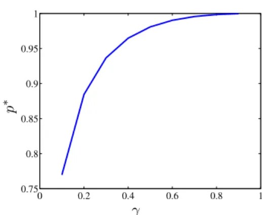
Proposition 4.4: For all fixed γ within the interval (0, 1), there exist p∗(γ) such that, for all p ∈ [p∗(γ), 1),
lim
|DCR|→+∞F(p, |DCR|, γ) = 0.
The proof is given in Appendix D.
This result can be interpreted as follows: for a given contrast level (any fixed γ), the a-contrario method enables to detect all change pixels when they represent a proportion of the image domain which is smaller than 1 − p∗(γ), provided that the
image is large enough. Figure 1 shows how this value p∗
evolves when γ is increasing (that is, when the contrast level is decreasing). Even though this result is asymptotic, practically it suggests to use as much data as possible when dealing with weak contrast images, rather than restricting to an extract of the area of interest.
0 0.2 0.4 0.6 0.8 1 0.75 0.8 0.85 0.9 0.95 1 PSfrag replacements γ p ∗
Fig. 1. Plot of the p∗ values obtained numerically for various values of
γ ∈(0, 1[.
V. ALGORITHM
From the definition of the NF A (Equation (11)), a subdo-main is detected as coherent with a given label map if it has a small NFA (and the smaller the NFA, the more coherent the subdomain). This latter depends on the size of the CR image domain, the number of labels, the size of the considered subdomain D, the standard-deviation of the naive model and the quadratic residue cumulated on this subdomain. Note that all NF A parameters are obtained directly from the data except the cumulated quadratic residue δ2(v
D) which depends on
the class means (a priori unknown). It is hence necessary to estimate the mean of each class before being able to compute the quadratic residues considered subdomain and then the corresponding NFA. The mean estimation and the detection itself are two linked problems as the quality of the estimation has a strong impact on the performance of the detection.
In general, the goal of usual estimation methods such as the mean square method is to maximize, for a given measure, the adequacy between a defined model and the data. Such methods are very sensitive to outliers as they aim at getting as close as possible to the whole sample. While dealing with change detection, change pixels play the role of outliers and, when numerous, they may dramatically bias the mean estimation. Robust methods such as M-estimators, LMedS or RANSAC have been introduced in order to face this problem. For instance, the M-estimators [39] enable a good estimation even when 50% of the pixels are outliers, by weighting the considered distance. However, the choice of the weight function is delicate.
The RANSAC (Random Sampling Consensus) method, pro-posed by [33], is based on the idea of using a sub-sample as small as possible and to fill it out with consistent data when possible, rather than using as many data as possible. More precisely, let us assume that a subsample of data is selected randomly and that parameters are estimated from this subsample. By chance, the considered subsample might happen not to contain any outlier, the parameter estimation is then correct and classifies the whole sample between correct and incorrect pixels. The RANSAC strategy is based on the idea that repeating this random sampling process a large amount of times must lead to a satisfactory solution. This approach, introduced in image analysis by [33], enables a
good parameter estimation even when outliers are numerous (about 50%). However, it is limited by the arbitrary choice of a threshold from which deciding that a subsample is in adequacy with the considered model.
In addition, minimizing the NFA ideally requires a combi-natory exploration of all image subdomains. However, such a thorough research is not conceivable in practice as, even for a very small image of 256 pixels, 2256
' 1.15·1077subdomains
should be analyzed. By noting that the best subdomains for the mean estimation are those minimizing the residues, we suggest to limit the exploration to the subdomains selected using a RANSAC-like strategy.
Hence, the detection algorithm we propose is based both on the random sampling strategy (cf. [33]) and on the NFA probabilistic criterion defined in Section III in order to free from the choice of an arbitrary decision threshold during the parameter estimation step meanwhile reducing the number of test subdomains. Such a collaboration has already been performed in [26] for rigidity detection and estimation of the fundamental matrix in stereoscopic vision.
The research of the minimum NF A can be accelerated using the following result.
Proposition 5.1: Given a fixed vector µ ∈ RL, define for
any D ⊂ DCR the square error δ2µ(vD) = Py∈Dr(y), with
r(y) = ¡v(y) − Pl∈Lαl(y)µ(l)
¢2
. If DCR = {yi}i=1...|DCR|
and the function i 7→ r(yi)is nondecreasing, then
arg min
D⊂DCR |D|=q
N F A(|D|, δµ(vD), σ) ={y1,· · · , yq}. (21)
Proof — Since r is sorted, for all D ∈ DCR such that |D| = q
we have δ2
µ(vD)≥ δµ2(v{y1,y2,··· ,yq}). As the NF A function
is non-decreasing with respect to δ, its minimum value is obtained for the subdomain {y1,· · · , yq}. ¤
Hence, if the quadratic residues are sorted with a non-decreasing order, considering each subdomain following the order of its residues is sufficient to minimize the NF A over all subdomains, for a given vector µ of label means.
Finally, in the case where a single CR image v is used, the algorithm is:
• Compute σ2, the CR image variance.
• Initialize δmin2 [], NF A[] and NF Amin to +∞. • Repeat N times
1) draw randomly |L| CR pixels, denoted by I = (x1,· · · , x|L|);
2) estimate the label mean vector µ from equations v(x) =X
l
αl(x)µl,
defined for x ∈ I;
3) compute r(x) = (v(x) − Plαl(y)µl)2, for x ∈
DCR;
4) sort DCR into a vector (xi)1≤i≤|DCR| by increasing
error r(xi);
5) initialize δ2=P|L|
i=0r(xi);
6) for each index i ∈ {|L| + 1, . . . , |DCR|}, – set δ2= δ2+ r(x
i);
– if δ2< δ2
min[i] then
∗ set δ2
min[i] = δ2;
∗ compute the corresponding NF A[i] value; ∗ if NF A[i] ≤ NF Amin, then
· set NF Amin= N F A[i];
· set D = {xk}k=1..i;
∗ end if
– end if
7) end for
• end repeat
This algorithm uses a HR label map and a CR image as inputs and returns the subdomain minimizing the NF A and the corresponding class means. The only parameter of the algorithm is the number of iterations (N). Due to RANSAC strategy, convergence requires a very high number of iterations (N = 100 000 in our experiments). However, this is not really a limiting factor as the computation time of each iteration is very fast (for instance, 100 000 iterations for change detection considering a HR classification of size 256 × 256 and a CR image of size 16 × 16 takes about 10s on a laptop).
VI. THE MULTITEMPORAL CASE
In the multitemporal case, different approaches may be cho-sen depending whether the application requires the detection of a spatio-temporal subdomain or a spatial subdomain. For instance, a sequential approach can be considered, comparing the minimum NF A values obtained for each image separately. Such an approach can be used in order to find the image of a time series which is the most coherent with the classification but it does not permit to detect a spatio-temporal subdomain. In practice, time series are rather used to analyse the temporal evolution of intensities and to enable the detection of spatio-temporal domains, which may be useful for applications where changes can occur at some dates without impacting other ones. Here, a vectorial approach is considered for the detection of a spatio-temporal subdomain of changes, assuming that all images of the time series are accurately registered. Denote T the set of acquisition dates of a time series. The a-contrario detection model presented Section III can be easily extended to time series, considering a spatio-temporal subdomain ω ∈ DCR× T . As a naive model, the CR time series is assumed
to be a random field of |DCR| × |T | independent Gaussian
random variables of zero-mean and variance σ2. From there,
the NF A is defined as in the monotemporal case by
N F A(|ω|, δ(vω), σ) = η(|ω|) · Γinc µ q 2, δ(vω)2 2σ2 ¶ , (22) where η(|ω|) = |DCR|·|T |·¡|DCR|ω||×|T | ¢ and q = |ω|−|L|×|T | Concerning the choice of the variance of the naive model, let us recall that, in the monotemporal case, taking the CR image variance as the variance of the naive model was justified by the fact that nothing should be detected in a white noise image. In the multitemporal case, setting the variance of the naive model to the variance of the CR time series does not ensure this property anymore as, in the case of high variance differences between dates within the time series, such a naive
model could detect noisy pixels as coherent. To avoid the detection of irrelevant subdomains, the intensity values are normalized by the image variance within each image and the variance of the naive model is set to 1. The multitemporal algorithm is very close to the monotemporal one but the fact that time series may contain missing data at different locations for each date must be taken into account in the research of the subdomain of changes. A simple possibility is to restrict the study to the set of pixels that are validated for all dates but this might considerably reduce the analysed domain. Instead, we propose to consider a restriction of DCR× T to the set of
valid pixels. More precisely, each pixel of the spatial domain is considered as a vector whose coordinates correspond to each of its valid dates. If a pixel is impacted by some changes at a given date, it will then be rejected for the whole series. In order to allow the comparison of subdomains of different size for each date, the cumulated residues are normalized by the number of valid dates, leading to a mean cumulated residue. Notice that with such an exploration, for a given pixel, the mean residue value is duplicated as many times as there are valid dates for this pixel thus enabling the detection of a spatial subdomain for which all valid dates are meaningfully coherent with the reference classification. From there, the same algorithm as in Section V can be used.
VII. RESULTS
In this section, the unique parameter of the a-contrario change detection method, ε, was set to 1 for all experiments so as to ensure less than 1 false alarms on average.
A. Experimental performances
Some experiments have been conducted in order to evaluate the performance and the limits of the method when the amount of change pixels varies in the image and when the objects of interest are small relative to the CR pixel size (i.e. when the resolution ratio is important). Simulated data have been used in order to enable a quantitative estimation of the performance while controling various impacting parameters.
First, let us focus on the robustness of the method when the amount of change pixels (or outliers) varies in the CR image. To that aim, a fixed resolution ratio of 16 × 16 has been considered and CR images containing 256 pixels have been simulated with an average contrast level. Change pixels have been introduced by corrupting the CR images with an impulse noise (random intensity values assigned to random pixels) impacting 0 to 100% of the image. The method has then been run for each image of the data set (500 tests) and the different types or detection error have been counted:
• the set oftrue positives is the set of all pixels which are
rightly detected as coherent with the reference classifica-tion. Conversely, the set of false positives is the set of all pixels which are wrongly detected as coherent with the reference classification (errors of type 1).
• the set of true negatives is the set of all pixels which
are rightly not detected as coherent with the reference classification (i.e. considered as changes). Conversely, the set of false negatives is the set of all pixels which are not
detected as coherent but should have been (errors of type 2).
Figure 2 shows the different types of errors obtained versus the number of change pixels. On both plots, each dot represents a test. Figure 2(a) represents the number of true positives (in green), the number of false negatives (in blue) and the number of pixels that effectively correspond to no change (in red, plotted just to increase the readibility) versus the actual number of change pixels in the image (the line y = 1 − x). Thus, the closer the true positives dots are to the no-change pixels dots, the more competitive is the detection.
(a) 0 50 100 150 200 250 0 50 100 150 200 250 no. of change pixels
# no-change # true positive # false negative (b) 0 50 100 150 200 250 0 50 100 150 200 250 no. of change pixels
# change # true negative # false positive
Fig. 2. Evolution of the performances versus the number of change pixels in an image with 256 pixels. On the left, the red dots on the diagonal stand for the actual no-change pixels in the test image, the number of pixels detected erroneously as changes (false negatives) is represented in blue, and the number of pixels accurately detected as no-change (true positives) is represented in green. On the right, the red dots on the diagonal stand for the change pixels, the number of pixels erroneously detected as no-change is represented in blue cross and, in green, the number of pixels detected as changes. The quality of the detection is thus shown as the closer the set of true positives gets to the set of no change pixels, the better is the detection performance.
Figure 2(b) represents the number of true negatives (in green), of false positives (in blue) and of actual change pixels (in red) versus the number of actual change pixels. It appears that the closer the true negatives dots are to the x = y line, the better are the detection performances. Besides, these two plots show the absence of detection only when the number of change pixels in the image represents more than about 80% of the CR image. Such performance is particularly high compared to the usual limitation threshold of 25% or 30% of change pixels found in the literature (cf. [23]). This result confirms the asymptotic theoretical result mentioned Section IV. Besides, the fact that the method is based on the control of the average number of false alarms (false positives) appears comparing
Figures 2(a) and 2(b) (plots in blue). Indeed, the number of false positives (Figure 2(b)) barely increases when the number of change pixels increases, whereas the number of false negatives (Figure 2(a)) increases more clearly with the number of change pixels.
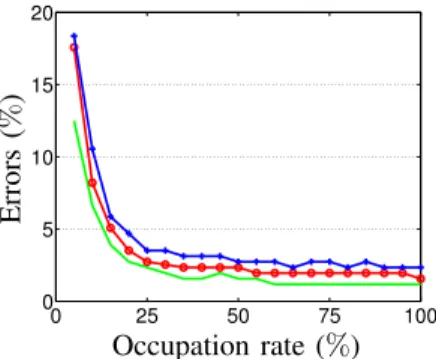
Finally, the performance of the method has been studied when the change areas only partially impact a CR pixel. Such case occurs whenever the change object of interest is smaller than the CR pixel. It is one of the main challenge addressed by the method. To that aim, a fixed average contrast level and a fixed global amount of change pixels of 20% are considered for the data set, and changes are simulated with a size varying from 0 to 100% of the CR pixel. Figure 3 presents the global error percentage obtained as a function of the percentage of changes within the CR pixel. It appears that the method is capable of detecting changes with less than 5% errors (median) as soon as their impacted surface represents less than 13% of the CR pixel, and with less than 3% errors when changes represents more than 25% of the CR pixel. The performance of the detection is barely increasing after this threshold.
0 25 50 75 100 0 5 10 15 20 PSfrag replacements Occupation rate (%) Errors (% )
Fig. 3. Errors of detection (% of the number of pixels in the image) obtained versus the occupation rate of changes within a CR pixel : 25, 50 and 75 percentiles (respectively in green, red and blue). Performances obtained for images simulated with 20% of change pixels and a resolution ratio of 16×16, showing that changes impacting more than 13% of a CR pixel are detected with less than 5% of error (in median).
B. Application to land cover change detection
In this section, a case of application to remotely sensed imagery is presented. Using Earth observation data, changes of interest are, typically, natural phenomena such as vegetation growth, flooding or fires and phenomena related to human ac-tivities such as urbanism, forest cuts, crop rotation or pollution. Here, a real time series of HR (SPOT 4) images of an area of intensive agricultural practice in the Danubian plain (Rumania, ADAM database1) has been considered. As no groundtruth on
changes was available, a HR classification has been derived from the HR time series and changes have been simulated either on the HR classification or on the CR image (obtained by averaging the real HR time series by blocks 16 × 16).
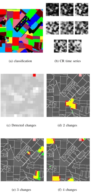
Figure 4 (a) shows the HR classification derived from the 8 HR real images (Fig. 4 (b)) and containing 10 labels
1The ADAM database (http://kalideos.cnes.fr) has been constituted in the
context of the ADAM project in order to assess the potential of spatial data assimilation techniques with agronomic models.
(using [40]). The change detection method applied to this classification and the corresponding CR time series with 8 dates enabled to validate the whole domain except the pixel in red Figure 4 (c). However this latter pixel shall not be considered as a false detection as it involves the quality of the classification rather than the change detection method in itself. We then artificially introduced different changes in the HR classification. First, in Figure 4, changes were introduced in the reference classification by replacing a random selection of segments label with another existing label. Figure 4(d) to (f) present several cases of such simulated changes and pixels detected as changes are presented in red in the CR domain. On the same image, the boundary of each segment is plotted in black, pixels corresponding to simulated changes are represented in green and those that were already detected in (c) are in pink. The small number of segments enables to visualize the impact area of segments of interest within CR pixels. Changes are well detected by the method, even when they impact a very small area of a CR pixel (Figure 4(d) and (f)).
We now aim at evaluating the interest of our approach relatively to state of the art methods. In the literature, most change detection methods apply to images having the same spatial resolution (see [18], [19]). In general, they assume a Markov Random Field model for the change detection image (as in [15], [16]), which is adapted only to the detection of ob-jects with a size greater than the pixel size (typically the field surface in our remote sensing application), or they boil down to an automatic thresholding of the difference image (e.g. [41]– [43]). As the spatial resolution we consider in this paper is generally too coarse relatively to the objects of interest, we focused on the sub-pixel change detection problem which cannot be compared directly to the previously mentionned methods. Alternately, few works are dedicated to the sub-pixel problem. We choose to compare our method to the IE method described in [23] as it considers a very similar problem (comparison of a CR series with a HR reference label map). In [23], change detection is performed through an alternate estimation of class means (pixel disaggregation problem) and pixel composition (supervised subpixel classification problem) removing pixels causing largest errors (assumed to correspond to changes). The weak points of such an approach are as follows. First, during the pixel disaggregation step, the number of considered pixels should be greater than the number of classes (in a ratio greater than two in order to get good estimations). Then, during the pixel composition estimation, the number of considered bands (e.g. the number of dates times the number of spectral bands) should be greater than the number of classes (also in a ratio greater than two if possible). Lastly, the number of change pixels should not be too important since they are present at the beginning of the iterative process (practically no more than 30% of the total number of pixels). Figure 5 shows the obtained results in the case of changes introduced the reference classification 5(a), as for Fig. 4. More precisely, our aim is to detect changes occuring in the CR 8-dates time series 4(c) referring to the HR 5-classes classification Fig. 5(a). Indeed, as the iterative estimation (IE) method needs more dates in the time series
(a) classification (b) CR time series
(c) Detected changes (d) 2 changes
(e) 3 changes (f) 4 changes
Fig. 4. Results obtained for changes introduced in the classification by a random choice of 3, 4 or 5 segments, to which are assigned random labels between 1 and L. Changes that have been simulated in the classification are represented in yellow when they are detected, green otherwise. Detected pixels that do not correspond to changes are represented in pink if they were already detected before the simulation of changes (cf. (c)) and in red otherwise. Globally, remark that simulated changes are well detected even when they impact a weak proportion of a CR pixel. On Figure (e), missed detections can be observed (to the right, in green).
than the number of classes in the classification, we had to reduce the number of classes to 5 so that the IE method performs well. The colour code for change and/or detected pixels is the same as in Fig. 4. This time, no pixel has been detected running our method (refered as NFA) for the CR time series Fig. 4(b) and the corresponding classification Fig. 5(a) before introducing some changes, showing that all CR pixels are coherent with the reference classification. Con-versely, Fig. 5(b) shows in red the pixels which are detected using IE for the same experiment. Hence, these four pixels
(a) classification (b) Detected changes
(c) 2 changes (NFA) (d) 2 changes (IE)
(e) 3 changes (NFA) (f) 3 changes (IE)
Fig. 5. Comparison of NFA and IE methods for changes introduced in the classification by a random choice of 2 and 3 segments, and a new label between 1 and L assigned to each chosen segment. Almost all changes are detected and almost no false alarm is obtained using the NFA whereas missed detections and false alarms are obtained with IE, thus confirming the high performance of the NFA.
are considered as not valid for the next change detection experiments using IE. Figures 5(c) and (d) present the results obtained respectively using the NFA and the IE methods when 2 changes have been introduced in the classification (in green) : using the NFA method, we obtain 7 true alarms (in yellow), 0 false alarm and 8 missed alarms (only one of which impacts the whole pixel) ; using the IE method, 3 true detections, 12 missed alarms have been obtained. Note that the two pixels in pink are not considered as false alarms as they were already detected in Fig.5(b). Figures 5(e) and (f) show the results of the NFA and IE for 3 other changes: 10 true detections, 1 false alarm and 3 missed detections can be observed using the NFA whereas only 3 true detections can be observed using the IE (and 6 false alarms, 10 missed detections). Through these
results, the better performance of the NFA compared to the IE appears clearly. In addition, as mentioned before, the case of application of the IE is much more limited than the NFA. Besides, the good control of the number of false alarms using the NFA is again proven.
Next, changes are simulated on the CR image, standing for wide area changes, whereas the previous experiments validated sub-pixel land cover change detection. To that aim, the HR classification Figure 6 (a) is considered as a reference and changes are simulated on the CR image Figure 6 (b) replacing the pixel values within two rectangular areas (see in the white areas Figure 6(c)) by the pixel values obtained on another part of the image, for another date. The method applied to Fig. 6 (a) and (b) enabled us to detect all red pixels Figure (c). The pixels in pink correspond to pixels that were already detected before the simulation of changes in Fig. 6 (b).
(a) classification
(b) Modified CR
im-age (c) Detected changes
Fig. 6. Detection of changes introduced in the CR image (b) corresponding to the HR classification (a) : detected changes are represented in red Figure (c) and the boundary of introduced changes is represented in white in the same image. Changes concern 5.46% of the CR pixels and 96.2% of the image had been validated before introducing changes. Detected pixels concerns 89.3% of the pixels, which is close to the expected 90.7%.
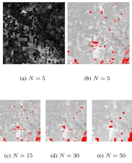
An important aspect of this method is the resolution ratio between HR and CR. The comparison of the results presented Figure 7 shows the robustness of the method with respect to the resolution ratio. Indeed, in a monotemporal context, the change detection method has been applied to the classification
shown on Figure 6 (a) and a corresponding HR image averaged by blocks of size 5 × 5 (Figure 7(b)), 15 × 15 (Figure 7(c)), 30× 30 (Figure 7(d)) and 50 × 50 (Figure 7(e)). Even though we cannot discuss the accuracy of the detected changes (as no groundtruth were available), notice that in these four cases, about 4.5% of the pixels are detected and that the spatial lo-cation of the detected pixels as non-coherent (in red) is stable, showing the good robustness of the method with respect to the resolution ratio. Moreover, as most methods in the literature are based on the analysis of the difference image, Figure 7(a) presents the difference image between the radiometric images acquired at the two dates which are considered for change detection Figure 7(b) to (e) thus illustrating the interest of using a classification instead of a radiometric image as a reference : the difference grey levels are very spread (difficult choice of a threshold) and many areas are characterized by large difference values but do not necessarily correspond to changes of interest.
(a) N = 5 (b) N = 5
(c) N = 15 (d) N = 30 (e) N = 50
Fig. 7. Change detection using the HR classification of Figure 6 (a) and a CR image with a resolution ratio (N) of 5×5, 15×15, 30×30 and 50×50. Detected pixels are presented in red, superimposed on the CR image used : the same areas are detected when the resolution ratio increases.
VIII. CONCLUSION
In this paper, a fully unsupervised method has been provided for sub-pixel change detection. The change detection problem has been considered comparing a CR time series to a HR clas-sification at a reference date. This formulation minimizes the required prior on the expected evolution, taking into account a reference classification rather than an image. Moreover, it allows the detection of sub-pixel changes.
The method we proposed is based on the definition of a coherence measure between a CR time series and the HR classification, using an a-contrario framework which does not require any a priori information. Indeed, rather than providing an a priori model for the data, the method is based on the
reject of a naive model (non-structured) by the observation of structured data. A theoretical analysis of this model underlined properties announcing its performances as functions of the image contrast level or of the amount of change pixels in the image.
In practice, utilizing this model requires the estimation of class means and the research of the spatio-temporal subdomain minimizing the NF A. To that aim, a stochastic algorithm using a RANSAC strategy has been used. It enables a robust estimation even when numerous pixels are outliers. Indeed, whereas existing methods are generally limited to less than 20% outliers in the image, this approach enables to override these limits showing good performances with up to 70% out-liers. Besides, simulations enabled an experimental assessment of the performances. In particular, it appeared that for an average contrast level, changes impacting more than 25% of a CR pixel are accurately detected as soon as less than 65% of the image is impacted.
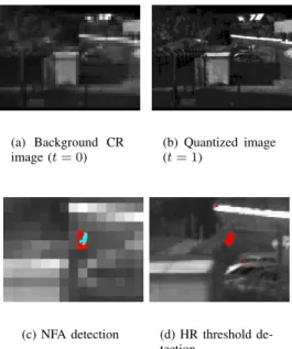
The multitemporal case has been discussed in particular as it implies to deal with the chronic issue of missing data. An adapted extension of the algorihm has been proposed, taking into account the fact that a time series often shows high variabilities between two dates. However, recall that this approach theoretically applies to any type of image series. Further studies and experiments will concern other cases of application using hyperspectral images or video sequences. As an instance, Fig. 8 shows some results obtained by testing our approach on an Infra-Red sequence acquired in the framework of video surveillance application (Safearound project). In this application, the CR image is the background image both for memory save and low-pass filtering of noise, and the HR image is the radiometric image just acquired. First, this latter HR image is quantized (in 10 grey levels Fig. 8(b)). Then the proposed algorithm can be applied directly. In Fig. 8(c), the intruder clambering up the wire fence is well detected (no missed alarm, no false detection) even if he impacts only partly two CR pixels. As a comparison, Fig. 8(d) corresponds to the result finding the best threshold on the difference image (between HR images) : the intruder is correctly detected but several false alarms (cars and hut roof) can also be observed, thus illustrating the interest of our method.
Lastly, the results obtained using pseudo-real data showed very good performance and robustness to the resolution ratio used. However, further validation on real time series with known changes are still to be performed, in order to analyse in particular the sensitivity of the model to other departures from the block average hypothesis. Moreover, this approach is based on the assumption of perfect image registration. Further work should focus on a registration sensitivity analysis as, in reality, registration is not perfect and the use of misregistred time series would lead to cumulated errors.
APPENDIXA THEOREM3.1
Using the a-contrario hypothesis denoted by H0(m), for
all m ∈ R|DCR|, the number of false alarms associated to a
(a) Background CR
image (t = 0) (b) Quantized image(t = 1)
(c) NFA detection (d) HR threshold de-tection
Fig. 8. Video surveillance using Infra-Red images. The background CR image (a) is an image of the sequence without any event of interest. In image (b), an intruder appears (quantized into 10 grey levels). The result of the NFA method (Image (c)) using (a) and (b) shows in (c) in red the CR detected pixels and in blue the track of the intruder (no false alarm, no missed detection). Image (d) presents in red the detected pixels using a thresholding method with HR images : the intruder is well detected but several false alarms can also be observed.
subdomain D of an image v is determined by
N F A(D, δ(vD), σ, m) = η(|D|) · f(q, δ(vD), σ, m), (23)
where η(|D|) = |DCR|¡|D|D|CR|
¢
, q = |D| − |L| (|L| being the number of labels) and, for all q ∈ N+
f (q, δ, σ, m) = 1 σq(2π)q2 Z Bq(δ) e−12 Pq i=1( xi−mi σ ) 2 dx1...dxq,
Bq(δ)being the ball of Rq with center 0 and radius δ.
Proof — From Proposition 3.1, specifying explicitly the NF A requires the calculation, for a given δ(vD), of the probability
PH
0[δ(VD)≤ δ(vD)]. (24)
Let AD = (αl(y))y∈D,l∈L be the matrix of label proportion
restricted to the subdomain D (matrix of size |D| × |L|). The residual error δ(VD) = min µ∈RL v u u t X y∈D Ã V (y)−X l∈L αl(y)µ(l) !2 (25)
can be interpreted as a distance from the vector VD to the
matrix AD image space denoted by ImAD. The minimal
distance is hence the orthogonal projection of VDon the space
(ImAD)⊥, i.e.
δ(VD) = min
µ∈RLkVD− ADµk = kp(ImAD)⊥(VD)k. (26)
According to Hypothesis H0, the vector VD follows a