Appendix
Litter decomposition driven by soil fauna, plant diversity and soil management in
urban gardens
Simon Tresch
1,2,3,∗, David Frey
3,4, Ren´ee-Claire Le Bayon
1,Andrea Zanetta
3,5, Frank Rasche
6, Andreas Fliessbach
2and Marco Moretti
31University of Neuchˆatel, Institute of Biology, Functional Ecology Laboratory, Rue Emile-Argand 11, 2000 Neuchˆatel, CH 2Research Institute of Organic Agriculture (FiBL), Department of Soil Sciences, Ackerstrasse 113, 5070 Frick, CH 3Swiss Federal Research Institute WSL, Biodiversity and Conservation Biology, Zuercherstrasse 111, 8903 Birmensdorf, CH 4ETHZ, Department of Environmental System Science, Institute of Terrestrial Ecosystems, Universitaetstrasse 16, 8092 Zurich, CH
5University of Fribourg, Department of Biology, Chemin du mus´ee 10, 1700 Fribourg, CH
6Institute of Agricultural Sciences in the Tropics (Hans-Ruthenberg-Institute), University of Hohenheim, Garbenstr. 13, 70599 Stuttgart, DE
Appendix A. Tables
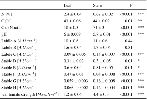
Table A.1: Trait measurements of Zea mays leaf and stem litter used for the decomposition experiment. For each litter type ten randomised samples were measured. Differences in traits were investigated with a non-parametrical Wilcoxon rank sum test.
Leaf
Stem
P
N [%]
2.4 ± 0.04
0.62 ± 0.02
<0.001
***
C [%]
43 ± 0.06
44 ± 0.07
0.01
**
C to N ratio
18 ± 0.3
71 ± 3
<0.001
***
pH
6 ± 0.009
5.7 ± 0.01
<0.001
***
Labile A [A.U.cm
−1]
10 ± 0.6
11 ± 0.6
0.44
Labile B [A.U.cm
−1]
1.6 ± 0.04
1.7 ± 0.04
0.31
Labile C [A.U.cm
−1]
0.09 ± 0.005
0.14 ± 0.007
<0.001
***
Stable D [A.U.cm
−1]
0.31 ± 0.03
0.5 ± 0.05
0.01
*
Stable E [A.U.cm
−1]
0.6 ± 0.04
0.81 ± 0.05
0.01
*
Stable F [A.U.cm
−1]
0.47 ± 0.01
0.04 ± 0.008
<0.001
***
Stable G [A.U.cm
−1]
0.059 ± 0.003
0.16 ± 0.008
<0.001
***
Stable H [A.U.cm
−1]
0.066 ± 0.002
0.12 ± 0.004
<0.001
***
leaf tensile strength [MegaNm
−2]
1.2 ± 0.06
4.4 ± 0.3
<0.001
***
Table A.2: Soil mesofauna extraction temperature values and time for the high temperature and moisture gradient MacFadyen extractor. Best extraction time and temperature values has been reviewed from the literature [12,13,1].
Time [d]
1
2
3
4
5
6
7
Table A.3: 19 substrates used for the assessment of the Community level physiological profile (CLPP) based on the MicroResp™ technique [3]. We dissolved 18 substrates in H2Odeminand added 25µl aliquots to deliver 30 mg of C-substrate per g of soil water for each well. Each substrate was measured in five technical replicates. The absorbance of the detection plate is measured at 570 nm after 5 hours of incubation at 20°C in the dark. The detection plate contains a pH sensitive dye (Cresol Red) which is dissolved in a solution with 150 mM potassium chloride (KCl) and 2.5 mM sodium bicarbonate (NaHCO3) in a matrix of 1% agarose gel. For the calibration equations 44 samples from five different soils together with four different quantities (10 g, 20 g, 30 g and 40 g) were amended with 0, 0.5, 2, 3, 5 and 10 mg of glucose or α-keto-glutaric acid per g soil. The substrates were dissolved in water so that 62.5µl per g soil was added to each sample. Samples without substrates received the same amount of water. The calibration was obtained in 100ml Schott bottles containing 4 wells of breakable microstrips filled with the detection gel. These microstrips were measured immediately before and after the incubation on a plate reader (MRX II TC, Dynex, USA) at 570 nm. The bottles were sealed and CO2evolution was measured on a gas chromatograph (7890A, Agilent Technologies, USA). The difference in absorbance between the first and the second measurement is then plotted against the log of CO2evolution measured by the gas chromatograph. The linear fit between measured log(CO2) concentrations [µgCO2− Cg−1h−1] was y= −4.67 + 2.90 with an R2of 0.87.
Compound category
Substrate
Amino acid
gamma-aminobutyric acid
alanine
aspartic acid
glutamine
leucine
cysteine
Amino sugar
glucosamine
Sugar
arabinose
galactose
glucose
fructose
Carboxylic acid
ascorbic acid
citric acid
malic acid
alpha-keto-glutaric acid
Phenolic acid
protocatechuic acid
vanillic acid
Hemicellulose
xylan
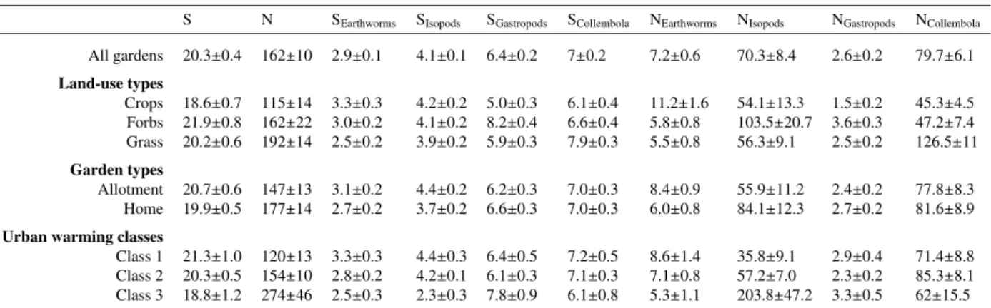
Table A.4: Descriptive statistics of biodiversity components per soil fauna taxa. Species and trait list used for the calculation of the biodiversity components are shown in Table A.5. Presented values are mean values with standard errors. S= species richness, N = abundance. All gardens n=168, crops n=46, forbs n=52, grass n=70, allotment n=82, home n=86, urban warming class 1 n=34, urban warming class 2 n=114, urban warming class 3 n=20.
S N SEarthworms SIsopods SGastropods SCollembola NEarthworms NIsopods NGastropods NCollembola
All gardens 20.3±0.4 162±10 2.9±0.1 4.1±0.1 6.4±0.2 7±0.2 7.2±0.6 70.3±8.4 2.6±0.2 79.7±6.1 Land-use types Crops 18.6±0.7 115±14 3.3±0.3 4.2±0.2 5.0±0.3 6.1±0.4 11.2±1.6 54.1±13.3 1.5±0.2 45.3±4.5 Forbs 21.9±0.8 162±22 3.0±0.2 4.1±0.2 8.2±0.4 6.6±0.4 5.8±0.8 103.5±20.7 3.6±0.3 47.2±7.4 Grass 20.2±0.6 192±14 2.5±0.2 3.9±0.2 5.9±0.3 7.9±0.3 5.5±0.8 56.3±9.1 2.5±0.2 126.5±11 Garden types Allotment 20.7±0.6 147±13 3.1±0.2 4.4±0.2 6.2±0.3 7.0±0.3 8.4±0.9 55.9±11.2 2.4±0.2 77.8±8.3 Home 19.9±0.5 177±14 2.7±0.2 3.7±0.2 6.6±0.3 7.0±0.3 6.0±0.8 84.1±12.3 2.7±0.2 81.6±8.9
Urban warming classes
Class 1 21.3±1.0 120±13 3.3±0.3 4.4±0.3 6.4±0.5 7.2±0.5 8.6±1.4 35.8±9.1 2.9±0.4 71.4±8.8 Class 2 20.3±0.5 154±10 2.8±0.2 4.2±0.1 6.1±0.3 7.1±0.3 7.1±0.8 57.2±7.0 2.3±0.2 85.3±8.1 Class 3 18.8±1.2 274±46 2.5±0.3 2.3±0.3 7.8±0.9 6.1±0.8 5.3±1.1 203.8±47.2 3.3±0.5 62±15.5
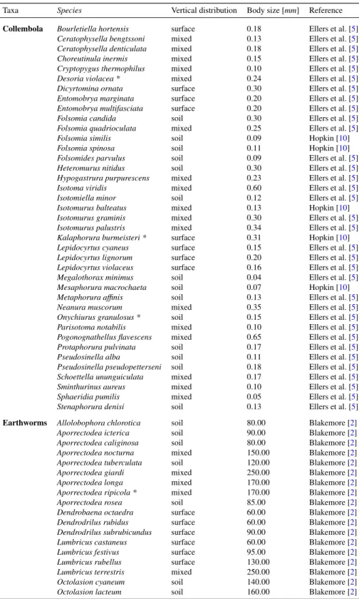
Table A.5: Species names and traits table. Species names were matched with Hinchliff et al. [9], while stars indicate that only the genus was found on the open tree of life data base [9]. Number of collembola species= 39, number of earthworm species = 18, number of gastropod species = 47 and number of ispod species= 16.
Taxa Species Vertical distribution Body size [mm] Reference
Collembola Bourletiella hortensis surface 0.18 Ellers et al. [5]
Ceratophysella bengtssoni mixed 0.13 Ellers et al. [5]
Ceratophysella denticulata mixed 0.18 Ellers et al. [5]
Choreutinula inermis mixed 0.15 Ellers et al. [5]
Cryptopygus thermophilus mixed 0.10 Ellers et al. [5]
Desoria violacea * mixed 0.24 Ellers et al. [5]
Dicyrtomina ornata surface 0.30 Ellers et al. [5]
Entomobrya marginata surface 0.20 Ellers et al. [5]
Entomobrya multifasciata surface 0.20 Ellers et al. [5]
Folsomia candida soil 0.30 Ellers et al. [5]
Folsomia quadrioculata mixed 0.25 Ellers et al. [5]
Folsomia similis soil 0.09 Hopkin [10]
Folsomia spinosa soil 0.11 Hopkin [10]
Folsomides parvulus soil 0.09 Ellers et al. [5]
Heteromurus nitidus soil 0.30 Ellers et al. [5]
Hypogastrura purpurescens mixed 0.23 Ellers et al. [5]
Isotoma viridis mixed 0.60 Ellers et al. [5]
Isotomiella minor soil 0.12 Ellers et al. [5]
Isotomurus balteatus mixed 0.13 Hopkin [10]
Isotomurus graminis mixed 0.30 Ellers et al. [5]
Isotomurus palustris mixed 0.34 Ellers et al. [5]
Kalaphorura burmeisteri * surface 0.31 Hopkin [10]
Lepidocyrtus cyaneus surface 0.15 Ellers et al. [5]
Lepidocyrtus lignorum surface 0.20 Ellers et al. [5]
Lepidocyrtus violaceus surface 0.16 Ellers et al. [5]
Megalothorax minimus soil 0.04 Ellers et al. [5]
Mesaphorura macrochaeta soil 0.07 Hopkin [10]
Metaphorura affinis soil 0.13 Ellers et al. [5]
Neanura muscorum mixed 0.35 Ellers et al. [5]
Onychiurus granulosus * soil 0.15 Ellers et al. [5]
Parisotoma notabilis mixed 0.10 Ellers et al. [5]
Pogonognathellus flavescens mixed 0.65 Ellers et al. [5]
Protaphorura pulvinata soil 0.17 Ellers et al. [5]
Pseudosinella alba soil 0.11 Ellers et al. [5]
Pseudosinella pseudopetterseni soil 0.18 Ellers et al. [5]
Schoettella ununguiculata mixed 0.17 Ellers et al. [5]
Sminthurinus aureus mixed 0.10 Ellers et al. [5]
Sphaeridia pumilis mixed 0.05 Ellers et al. [5]
Stenaphorura denisi soil 0.13 Ellers et al. [5]
Earthworms Allolobophora chlorotica soil 80.00 Blakemore [2]
Aporrectodea icterica soil 90.00 Blakemore [2]
Aporrectodea caliginosa soil 80.00 Blakemore [2]
Aporrectodea nocturna mixed 150.00 Blakemore [2]
Aporrectodea tuberculata soil 120.00 Blakemore [2]
Aporrectodea giardi mixed 250.00 Blakemore [2]
Aporrectodea longa mixed 170.00 Blakemore [2]
Aporrectodea ripicola * mixed 170.00 Blakemore [2]
Aporrectodea rosea soil 85.00 Blakemore [2]
Dendrobaena octaedra surface 60.00 Blakemore [2]
Dendrodrilus rubidus surface 60.00 Blakemore [2]
Dendrodrilus subrubicundus surface 90.00 Blakemore [2]
Lumbricus castaneus surface 60.00 Blakemore [2]
Lumbricus festivus surface 95.00 Blakemore [2]
Lumbricus rubellus surface 130.00 Blakemore [2]
Lumbricus terrestris mixed 250.00 Blakemore [2]
Octolasion cyaneum soil 140.00 Blakemore [2]
Taxa Species vertical distribution body size [mm] Reference
Gastropoda Acicula lineata surface 3.75 Falkner et al. [6]
Aegopinella minor mixed 10.00 Falkner et al. [6]
Aegopinella nitens mixed 10.00 Falkner et al. [6]
Aegopinella pura surface 3.75 Falkner et al. [6]
Arion surface 80.00 Falkner et al. [6]
Boettgerilla pallens soil 60.00 Falkner et al. [6]
Carychium tridentatum mixed 1.25 Falkner et al. [6]
Cecilioides acicula soil 53.10 Falkner et al. [6]
Cepaea hortensis surface 22.50 Falkner et al. [6]
Cepaea nemoralis surface 22.50 Falkner et al. [6]
Cepaea surface 22.50 Falkner et al. [6]
Cochlicopa lubrica mixed 10.00 Falkner et al. [6]
Columella edentula surface 3.75 Falkner et al. [6]
Deroceras surface 30.00 Falkner et al. [6]
Discus rotundatus mixed 10.00 Falkner et al. [6]
Fruticicola fruticum surface 19.40 Falkner et al. [6]
Galba truncatula surface 2.75 Falkner et al. [6]
Helix pomatia surface 22.50 Falkner et al. [6]
Hygromia cinctella surface 10.00 Falkner et al. [6]
Laciniaria plicata mixed 10.00 Falkner et al. [6]
Limax maximus surface 150.00 Falkner et al. [6]
Macrogastra attenuata mixed 17.50 Falkner et al. [6]
Monachoides incarnatus mixed 13.10 Falkner et al. [6]
Nesovitrea hammonis mixed 3.75 Falkner et al. [6]
Oxychilus cellarius soil 10.00 Falkner et al. [6]
Oxychilus draparnaudi mixed 13.10 Falkner et al. [6]
Oxychilus * mixed 11.55 Falkner et al. [6]
Paralaoma servilis mixed 1.25 Falkner et al. [6]
Punctum pygmaeum mixed 1.25 Falkner et al. [6]
Pupilla muscorum surface 3.75 Falkner et al. [6]
Succinea putris surface 13.13 Falkner et al. [6]
Succinea oblonga mixed 10.00 Falkner et al. [6]
Tandonia budapestensis surface 35.00 Falkner et al. [6]
Trochulus clandestinus mixed 10.00 Falkner et al. [6]
Trochulus sericeus surface 10.00 Falkner et al. [6]
Trochulus mixed 10.00 Falkner et al. [6]
Vallonia costata mixed 2.50 Falkner et al. [6]
Vallonia excentrica surface 1.88 Falkner et al. [6]
Vallonia pulchella mixed 2.50 Falkner et al. [6]
Vallonia mixed 2.29 Falkner et al. [6]
Vertigo antivertigo surface 1.25 Falkner et al. [6]
Vertigo pusilla mixed 1.25 Falkner et al. [6]
Vertigo pygmaea mixed 1.25 Falkner et al. [6]
Vertigo mixed 1.25 Falkner et al. [6]
Vitrea contracta soil 2.50 Falkner et al. [6]
Vitrea crystallina mixed 3.75 Falkner et al. [6]
Vitrinobrachium breve soil 3.75 Falkner et al. [6]
Isopoda Androniscus roseus soil 0.35 Vandel [20]
Armadillidium nasatum surface 2.05 Vandel [20]
Armadillidium versicolor surface 1.75 Vandel [20]
Armadillidium vulgare surface 1.73 Vandel [20]
Cylisticus convexus soil 1.35 Vandel [20]
Haplophthalmus danicus soil 0.40 Vandel [20]
Haplophthalmus mengei soil 0.30 Vandel [20]
Hyloniscus riparius soil 0.80 Vandel [20]
Ligidium hypnorum surface 0.87 Vandel [20]
Oniscus asellus surface 1.63 Vandel [20]
Philoscia muscorum surface 1.06 Vandel [20]
Platyarthrus hoffmannseggii soil 0.30 Vandel [20]
Porcellio scaber surface 1.51 Vandel [20]
Porcellionides pruinosus mixed 1.05 Vandel [20]
Trachelipus rathkii surface 1.40 Vandel [20]
Table A.6: Management questions asked of all 85 participating urban gardeners of this study. Management intensity index was calculated as a scaled sum (divided by the number of questions) of all 26 garden management questions on a five level Likert scale. For the land-use type grass we considered nine questions: MowGrass, FstCutGrass, FertGrass, WaterGrass, CareGrass, PestGrass, FlowerIslands, Weeds, Leaves. For forbs ten questions: FertForbs, WaterForbs, PestForbs, DiggingForbs, ForkForbs, CutTrees, PestTrees, Leaves, DrySticks, Weeds and for crops eleven questions: FertCrops, WaterCrops, PestCrops, CropRotate, MixCult, Mulch, GreenFert, DiggingCrops, ForkCrops, DrySticks, Weeds. Higher factor levels indicate higher management intensity. Questions were originally asked in German.
PestGrass PestForbs PestCrops
How often do you use pesticides, fungicides or herbicides to protect your lawn?
How often do you use pesticides, fungicides or herbicides (without slug pellets) to pro-tect your flowers?
How often do you use pesticides, fungicides or herbicides (without slug pellets) to pro-tect your vegetables?
Never (1) Never (1) Never (1)
Less than once per year (2) Less than once per year (2) Less than once per year (2) 1 to 3 times per year (3) 1 to 3 times per year (3) 1 to 3 times per year (3) 4 to 10 times per year (4) 4 to 10 times per year (4) 4 to 10 times per year (4) More than 10 times per year (5) More than 10 times per year (5) More than 10 times per year (5)
FertGrass FertCrops FertForbs
How often do you use fertilisers for your lawn?
How often do you use fertilisers for your vegetables?
How often do you use fertilisers for your flowers?
Never (1) Never (1) Never (1)
4 to 5 times per year (2) 2 to 3 times per year (2) 2 to 3 times per year (2)
2 to 3 times per year (3) Once a year (3) Once a year (3)
once a year (4) 2 to 3 times per year (4) 2 to 3 times per year (4)
More than once a year (5) More than three per year (5) More than three per year (5)
Weeds PestTrees Leaves
How often do you remove most of the weeds in your garden?
How often do you use insecticides, fungi-cides or herbifungi-cides to protect our trees and shrubs?
How often do you remove most of the leaves in your garden?
Never (1) Never (1) Never (1)
Rarely (2) Less than once a year (2) Spring (2)
Sometimes (3) 1 to 3 times per year (3) Autumn (3)
Often (4) 4 to 10 times per year (4) Every 2 to 3 weeks (4)
Very often (5) More than 10 times per year (5) Weekly in autumn (5)
MowGrass MixCult FlowerIslands
How often do you mow your lawn per year? Do you follow the principle of mixed culti-vation (planting different varieties of vegeta-bles and/or flowers in the same cultivation plot)?
Do you leave islands of flowers when you mow your lawn?
1 to 2 (1) Never (5) Never (5)
3 to 4 (2) Rarely (4) Rarely (4)
5 to 8 (3) Sometimes (3) Sometimes (3)
9 to 20 (4) Mostly (2) Mostly (2)
WaterGrass WaterCrops WaterForbs How often do you water your lawn? How often do you water your vegetable
beds?
How often do you water your flower beds?
Never (1) Never (1) Never (1)
When dry (2) When dry (2) When dry (2)
once a week (3) once a week (3) once a week (3)
twice a week (4) twice a week (4) twice a week (4)
More than twice a week (5) More than twice a week (5) More than twice a week (5)
CareGrass DiggingForbs DiggingCrops
How often do you scarify your lawn (includ-ing reseed(includ-ing)
How often do you till your soil in the flower beds?
How often do you till your soil in the veg-etable beds?
Never (1) Never (1) Never (1)
Every 6 to 10 years (2) Every 3 years or less (2) Every 3 years or less (2)
Every 4 to 5 years (3) Every two years (3) Every two years (3)
Every 2 to 3 years (4) Once per year (4) Once per year (4)
Annually (5) More than once per year (5) More than once per year (5)
DrySticks FstCutGrass Mulch
Do you leave withered flowers and sticks during the winter in your garden?
When is the first time point of cutting your lawn?
Do you use organic material (mulch) to cover your vegetable beds?
Never (5) April (5) Never (5)
Rarely (4) May (4) Rarely (4)
Sometimes (3) Start June (3) Sometimes (3)
Mostly (2) End June (2) Mostly (2)
Always (1) After June (1) Always (1)
CropRotate GreenFert WeedingHerbicide
Do you consider changing flower beds (crop rotation) for the vegetables grown annually?
Do you grow plants for green manure? Do you use commercial herbicides?
Never (5) Never (5) No (0)
Rarely (4) Rarely (4) Yes (1)
Sometimes (3) Sometimes (3)
Mostly (2) Mostly (2)
Always (1) Always (1)
ForkForbs ForkCrops CutTrees
How often do you loosening your soil with a fork without turning it around (or milling)?
How often do you loosening your soil with a fork without turning it around (or milling)?
How often do you cut most of your forbs and trees?
More than once per year (5) More than once per year (5) More than once per year (5)
Once per year (4) Once per year (4) Once a year (4)
Every 2 years or less (3) Every 2 years or less (3) Every 2 years (3) Every 3 years or less (2) Every 3 years or less (2) Every 3 to 5 years(2)
Table A.7: Model selection based on goodness of fit statistics for LMEM, the widely applicable information criterion (WAIC), a Bayesian version of the AIC [21] and explained variance of the fixed effects R2
Marginaland including the random effect and the fixed effects R2Conditional. Model
1 included the selected biodiversity indices species richness (S), species evenness (EShannon), phylogenetic species variability (PSV), trait even distribution (TED) and the garden ID as random effect : lmer(log(100 − response + 1) ∼ S + EShannon+ PS V + T ED + (1|Garden ID), REML = F). Model 2 included garden land-use and garden type in addition to predictor variables of the previous model 1. For model 3 we included the multiple substrate-induced respiration rate (MSIR) as a measure for microbial activity. For model 4 we added urban warming. All fixed effects have been standardised (mean=0, standard deviation=1). R2based on fixed and random effects were calculated according to Nakagawa and Schielzeth [14].
Litter type
models
WAIC
R
2Marginal
R
2ConditionalLeaf 4mm
model 1
561.6 ± 11.4
0.07
0.30
model 2
529.8 ± 12.2
0.20
0.53
model 3
528.0 ± 12.2
0.22
0.54
model 4
523.0 ± 13.9
0.26
0.55
Stem 4mm
model 1
-137.0 ± 17.7
0.11
0.17
model 2
-200.2 ± 15.9
0.37
0.61
model 3
-203.4 ± 16.5
0.39
0.62
model 4
-203.4 ± 16.5
0.43
0.63
Leaf 1mm
model 1
365.1 ± 27.6
0.11
0.11
model 2
361.7 ± 31.3
0.16
0.19
model 3
358.1 ± 29.6
0.19
0.24
model 4
359.4 ± 29.4
0.19
0.24
Stem 1mm
model 1
-86.1 ± 26.00
0.13
0.13
model 2
-129.8 ± 23.6
0.35
0.54
model 3
-129.5 ± 24.0
0.35
0.54
model 4
-139.2 ± 22.8
0.41
0.56
Table A.8: Litter decomposition models for leaf and stem litter types and 1 and 4 mm mesh sizes. LMEM fixed effects were calculated using a simulated Bayesian inference posterior distribution. Bold numbers indicate significant fixed effects, with credible intervals not crossing zero. Number of observations for 4 mm litter bags n=154 and for 1mm litter bags n=122, due to missing litter bags from the garden sites. Garden ID was set as random factor. LMEM model: lmer(log(100 − decomposition+ 1) ∼ MS IR + S + ES hannon+ PS V + T ED + urban warming + land use types + garden types+ (1|Garden ID)). EShannon: Shannon evenness, MSIR: Multiple substrate-induced respiration of microorganisms, PSV: Phylogenetic species variability, S: Soil fauna species richness, TED: Trait even distribution.
Leaf 4mm [log(g)] Stem 4mm [log(g)] Fixed effects 50% (97.5%; 2.5%) 50% (97.5%; 2.5%) MSIR 0.24 (0.48; 0.01) 0.03 (0.05; 0.01) S 0.29 (0.53; 0.04) 0.01 (0.04;-0.01) EShannon 0.13 (0.40;-0.14) 0.01 (0.02;-0.03) PSV -0.03 (0.20;-0.25) 0.01 (0.02;-0.02) TED -0.05 (0.17;-0.26) -0.01 (0.01;-0.03) Urban warming 0.45 (0.76; 0.14) 0.04 (0.07; 0.01) Land-use types: forbs 0.35 (0.92;-0.22) 0.06 (0.11; 0.01) Land-use types: grass 1.10 (1.60; 0.61) 0.16 (0.21; 0.12) Garden types: home 0.00 (0.62;-0.61) 0.04 (0.09;-0.02)
Leaf 1mm [log(g)] Stem 1mm [log(g)] Fixed effects 50% (97.5%; 2.5%) 50% (97.5%; 2.5%) MSIR 0.11 (0.23;-0.01) 0.03 (0.06; 0.01) S -0.10 (0.03;-0.22) 0.03 (0.06; 0.01) EShannon -0.03 (0.09;-0.15) 0.03 (0.06; 0.01) PSV -0.11 (0.01;-0.24) -0.02 (0.01;-0.06) TED 0.09 (0.20;-0.02) 0.01 (0.03;-0.02) Urban warming 0.10 (0.22;-0.03) 0.06 (0.10; 0.03) Land-use types: forbs 0.03 (0.33;-0.27) 0.08 (0.15; 0.01) Land-use types: grass 0.34 (0.64; 0.03) 0.17 (0.25; 0.09) Garden types: home 0.09 (0.34;-0.17) 0.01 (0.09;-0.06)
T able A.9: Litter decomposition grouped by g arden land-use types, management and urban w arming classes (A-D). T ea bag inde x (TBI) decomposition is described in T resch et al. [ 18 ]. Question disturbance is related to the combined management answers (yes /no) of major soil disturbances (”DiggingV eg”, ”DiggingFlo wer”, ”CareLa wn”); pesticides is related to the use of pesticides (”PestLa wn”, ”PestV eg”, ”PestFlo wer”, ”PestT rees”, ”W eedingHerbicide”); compost is related to the use of compost (”FertLa wnCompost”, ”FertV egCompost”, ”FertFlo werCompost”) and w ater to the application of additional w ater (”W aterLa wn”, ”W aterV eg”, ”W aterFlo wer”). Indi vidual management questions can be found in T able A.6. Urbanisation intensity w as in v estig ated as urban w arming classes. Decomposition [%] is gi v en as a mean decomposition rate including standard error v alues. Di ff erences were in v estig ated with a non-parametrical W ilcoxon rank sum test and if more than tw o groups with a LMEM with g arden ID as random eff ect and analysed with a Bayesian approach including means and 95 % credible interv als of the Bayesian inference posterior distrib utions follo wing K orner -Nie v er gelt et al. [ 11 ]. Significant v alues are bold printed. A Fix ed eff ects [log(g)] Litter type N Decomposition [%] 50% 97.5% 2.5% Leaf 4mm 69 79.59 ± 2.21 Stem 4mm 62 37.89 ± 0.84 -2.04 -1.82 -2.28 Leaf 1mm 90 61.15 ± 1.95 Stem 1mm 65 40.07 ± 0.96 -0.63 -0.51 -0.76 Leaf 1mm 90 61.15 ± 1.95 Leaf 4mm 69 79.59 ± 2.21 1.37 1.61 1.12 Stem 1mm 65 40.07 ± 0.96 Stem 4mm 62 37.89 ± 0.84 -0.04 -0.01 -0.07 B Decomposition per land-use type Leaf 4mm Stem 4mm Leaf 1mm Stem 1mm TBI gr een tea TBI rooibos tea Land-use Fix ed eff ects [log(g)] Fix ed eff ects [log(g)] Fix ed eff ects [log(g)] Fix ed eff ects [log(g)] Fix ed eff ects [log(g)] Fix ed eff ects [log(g)] types N Decomposition [%] 50% 97.5% 2.5% N Decomposition [%] 50% 97.5% 2.5% N Decomposition [%] 50% 97.5% 2.5% N Decomposition [%] 50% 97.5% 2.5% N Decomposition [%] 50% 97.5% 2.5% N Decomposition [%] 50% 97.5% 2.5% crops 31 61.79 ± 5.57 31 30.45 ± 1.88 29 45.08 ± 5.33 28 29.98 ± 3.06 39 57.86 ± 0.67 39 29.28 ± 0.53 forbs 33 80.66 ± 3.52 0.7 1.26 0.15 34 37.89 ± 1.20 0.11 0.16 0.06 29 56.23 ± 3.54 0.17 0.46 -0.12 27 39.09 ± 1.55 0.13 0.2 0.05 45 58.64 ± 0.60 0.01 0.06 -0.04 45 29.5 ± 0.54 0.034 0.024 -0.017 grass 30 90.54 ± 1.76 1.34 1.83 0.84 36 42.82 ± 0.88 0.19 0.24 0.15 43 69.63 ± 2.19 0.56 0.82 0.29 31 46.00 ± 0.96 0.25 0.31 0.18 59 60.31 ± 0.66 0.06 0.11 0.02 59 29.48 ± 0.45 0.033 0.023 -0.017
C Decomposition per urban warming class Leaf 4mm Stem 4mm Leaf 1mm Stem 1mm TBI gr een tea TBI rooibos tea Urban warming Fix ed eff ects [log(g)] Fix ed eff ects [log(g)] Fix ed eff ects [log(g)] Fix ed eff ects [log(g)] Fix ed eff ects [log(g)] Fix ed eff ects [log(g)] classes N Decomposition [%] 50% 97.5% 2.5% N Decomposition [%] 50% 97.5% 2.5% N Decomposition [%] 50% 97.5% 2.5% N Decomposition [%] 50% 97.5% 2.5% N Decomposition [%] 50% 97.5% 2.5% N Decomposition [%] 50% 97.5% 2.5% Class 1 27 70.90 ± 5.26 25 33.68 ± 2.09 24 53.6 ± 6.08 23 34.29 ± 2.82 29 57.33 ± 0.70 29 28.59 ± 0.65 Class 2 50 79.85 ± 2.77 0.63 1.28 -0.01 55 38.05 ± 0.99 0.07 0.13 0.01 61 59.4 ± 2.38 0.02 0.31 -0.26 47 40.01 ± 1.28 0.09 0.17 0.01 98 59.36 ± 0.47 0.05 0.1 0.01 98 29.51 ± 0.35 0.013 0.033 -0.07 Class 3 12 91.92 ± 2.84 1.32 2.22 0.41 15 43.71 ± 1.52 0.15 0.24 0.07 10 73.4 ± 5.06 0.49 0.97 0.01 9 52.15 ± 3.25 0.32 0.45 0.18 16 60.83 ± 1.30 0.09 0.16 0.01 16 30.50 ± 0.81 0.027 0.057 -0.03 D Decomposition per garden management Management Leaf 4mm Stem 4mm Leaf 1mm Stem 1mm TBI gr een tea TBI rooibos tea question gr oup N Decomposition [%] P N Decomposition [%] P N Decomposition [%] P N Decomposition [%] P N Decomposition [%] P N Decomposition [%] P disturbance no 33 85.39 ± 2.73 0.04 * 40 40.83 ± 1.08 0.01 ** 42 63.7 ± 3.12 0.08 30 42.41 ± 1.26 0.06 61 59.66 ± 0.59 0.16 61 29.77 ± 0.44 0.37 yes 48 75.56 ± 3.18 53 35.85 ± 1.16 53 56.13 ± 3.00 46 37.87 ± 1.80 82 58.71 ± 0.51 82 29.18 ± 0.38 pesticides no 44 77.92 ± 3.12 0.54 52 37.16 ± 1.15 0.34 58 59.34 ± 3.00 0.60 45 39.26 ± 1.57 0.48 81 59.05 ± 0.54 0.74 81 29.77 ± 0.37 0.28 yes 40 81.74 ± 3.09 38 38.83 ± 1.21 40 59.27 ± 3.09 34 40.62 ± 1.77 62 59.20 ± 0.56 62 28.99 ± 0.45 compost no 33 76.52 ± 3.86 0.24 35 37.84 ± 1.44 0.99 33 59.50 ± 3.75 0.80 27 40.67 ± 1.77 0.72 49 59.37 ± 0.66 0.69 49 28.99 ± 0.53 0.18 yes 52 81.21 ± 2.70 53 37.92 ± 1.03 59 59.22 ± 2.72 50 39.36 ± 1.53 94 58.98 ± 0.48 94 29.67 ± 0.34 w ater no 8 88.69 ± 4.14 0.97 8 38.62 ± 2.22 0.94 6 60.67 ± 6.75 0.60 5 43.00 ± 1.87 0.78 8 59.65 ± 1.39 0.56 8 29.52 ± 1.10 0.99 yes 66 79.08 ± 2.32 62 37.85 ± 0.87 75 59.24 ± 2.29 58 39.61 ± 1.24 135 59.08 ± 0.40 135 29.43 ± 0.30 E Decomposition per garden land-use type and management Management Land-use Leaf 4mm Stem 4mm Leaf 1mm Stem 1mm TBI gr een tea TBI rooibos tea question types Gr oup N Decomposition [%] P N Decomposition [%] P N Decomposition [%] P N Decomposition [%] P N Decomposition [%] P N Decomposition [%] P disturbance crops no 14 68.23 ± 8.44 0.45 13 35.33 ± 2.71 0.07 13 51.54 ± 8.95 0.26 12 35.58 ± 3.68 0.09 14 57.94 ± 0.88 0.67 14 30.32 ± 0.93 0.24 yes 20 58.08 ± 7.33 23 27.63 ± 2.39 17 40.66 ± 6.57 17 26.16 ± 4.36 25 57.81 ± 0.94 25 28.70 ± 0.62 forbs no 15 88.76 ± 3.20 0.02 * 16 41.57 ± 1.25 0.01 ** 16 63.94 ± 4.55 0.05 * 14 43.19 ± 1.45 0.01 ** 23 59.57 ± 0.79 0.10 23 29.49 ± 0.76 0.88 yes 21 73.20 ± 5.75 21 34.50 ± 1.77 15 48.97 ± 4.85 15 35.24 ± 2.34 22 57.66 ± 0.87 22 29.52 ± 0.79 grass no 13 92.88 ± 1.87 0.58 20 43.56 ± 1.59 0.33 17 71.05 ± 2.81 0.81 16 46.05 ± 0.97 0.82 24 60.74 ± 1.16 0.79 24 29.73 ± 0.67 0.62 yes 21 89.07 ± 2.62 30 42.36 ± 1.04 31 68.73 ± 3.13 24 45.97 ± 1.46 35 60.01 ± 0.80 35 29.32 ± 0.61 pesticides crops no 18 61.48 ± 7.89 0.98 20 29.96 ± 2.46 0.52 19 42.55 ± 7.27 0.65 21 29.07 ± 3.82 0.56 23 57.84 ± 0.98 0.79 23 29.43 ± 0.71 0.94 yes 15 62.28 ± 7.50 14 31.22 ± 3.00 11 49.91 ± 7.12 10 31.73 ± 5.31 16 57.89 ± 0.89 16 29.07 ± 0.81 forbs no 19 79.37 ± 4.67 0.46 21 36.87 ± 1.51 0.29 22 59.63 ± 4.57 0.06 21 39.89 ± 2.03 0.22 26 57.76 ± 0.67 0.15 26 30.17 ± 0.63 0.12 yes 17 82.18 ± 5.44 20 39.09 ± 1.94 10 48.40 ± 4.47 9 37.25 ± 2.07 19 59.84 ± 1.05 19 28.58 ± 0.93 grass no 20 88.91 ± 2.54 0.34 27 42.69 ± 1.33 0.80 26 70.87 ± 2.63 0.73 21 45.92 ± 1.38 0.59 32 60.97 ± 0.96 0.35 32 29.69 ± 0.60 0.68 yes 18 92.52 ± 2.39 23 42.98 ± 1.12 23 68.08 ± 3.71 19 46.10 ± 1.34 27 59.52 ± 0.90 27 29.24 ± 0.68 compost crops no 5 52.00 ± 20.5 0.89 5 26.40 ± 8.32 0.56 4 39.38 ± 16.7 0.65 4 26.88 ± 10.0 0.78 5 56.27 ± 1.59 0.31 5 29.10 ± 1.39 0.79 yes 29 63.15 ± 5.77 27 31.01 ± 1.86 26 45.89 ± 5.71 25 30.43 ± 3.26 34 58.09 ± 0.74 34 29.31 ± 0.58 forbs no 18 74.91 ± 6.10 0.17 20 37.00 ± 1.99 0.88 12 51.58 ± 6.56 0.50 10 38.54 ± 3.05 0.74 21 59.58 ± 0.97 0.11 21 29.03 ± 0.78 0.46 yes 19 85.94 ± 3.57 23 38.70 ± 1.43 19 59.25 ± 3.99 19 39.45 ± 1.67 24 57.81 ± 0.71 24 29.92 ± 0.76 grass no 18 83.17 ± 3.85 0.02 * 20 41.02 ± 1.49 0.09 20 68.24 ± 3.68 0.43 19 44.62 ± 1.17 0.23 23 59.84 ± 1.02 0.61 23 28.93 ± 0.84 0.20 yes 18 95.20 ± 1.02 27 43.96 ± 1.07 29 70.52 ± 2.75 22 46.88 ± 1.38 36 60.60 ± 0.88 36 29.84 ± 0.50 w ater crops no 0 0 0 0 0 0 yes 31 61.79 ± 5.57 31 30.45 ± 1.88 29 45.08 ± 5.33 28 29.98 ± 3.06 39 57.86 ± 0.67 39 29.28 ± 0.53 forbs no 5 92.50 ± 5.14 0.38 5 40.40 ± 2.00 0.36 3 66.83 ± 13.5 0.47 3 44.50 ± 3.33 0.21 5 61.31 ± 1.45 0.07 5 30.56 ± 1.56 0.49 yes 30 79.28 ± 3.84 33 37.59 ± 1.32 26 55.17 ± 3.68 25 38.55 ± 1.65 40 58.30 ± 0.64 40 29.37 ± 0.58 grass no 3 82.33 ± 6.33 0.09 3 35.67 ± 5.09 0.14 3 54.50 ± 2.52 0.03 * 3 41.50 ± 2.02 0.14 3 56.88 ± 2.23 0.20 3 27.78 ± 0.89 0.34 yes 28 90.96 ± 1.82 35 43.19 ± 0.88 41 70.52 ± 2.25 29 46.26 ± 1.00 56 60.49 ± 0.68 56 29.58 ± 0.47
Table A.10: Estimated LMEM coefficients of different response variables and fixed effect variables (A-C). Garden ID was set as random effect in all models. Given are the mean, the 2.5% and the 97.5% quantiles of the Bayesian posterior distribution. Bold numbers indicate significant fixed effects, with credible intervals not crossing zero [11].
A
Response variables
Fixed e
ffects
Forbs vs. Crops
Grass vs. Crops
Plant species richness
-0.28 (-4.0;3.4)
-3.57 (-6.9;-0.2)
B
Response variables
Fixed effects
C
micBacteria
Fungi
MSIR [
µgCO
2-Cg
-1h
-1]
2.3e-02 (1.5e-02;3.1e-02)
6.1e-09 (1.9e-09;1.0e-08)
-4.3e-07 (-9.4e-07;9.7e-08)
C
Response variables
Fixed e
ffects
Urban warming
Forbs vs. Crops
Grass vs. Crops
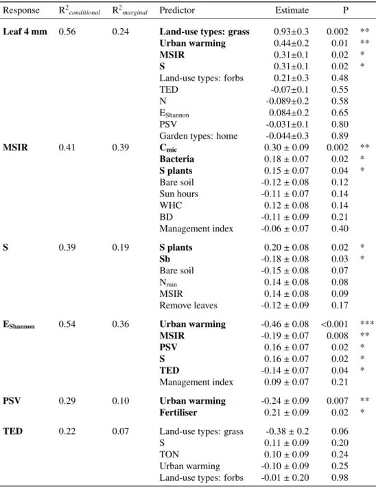
Table A.11: Alternative SEM including the effect of soil fauna abundance, as a proxy for soil fauna biomass, on litter decomposition (leaf litter 4 mm). SEM model goodness-of-fit outputs decreased in comparison to the original SEM (Table 4), with an increased AICc and a decreased P-value: AICc=356.8, Fisher’s C=175.9, P-value=0.25. Marginal R2based on fixed effects and conditional R2based on fixed and random effects. Significant paths are highlighted in bold. BD: Soil bulk density, Cmic: Microbial biomass carbon, EShannon: Shannon evenness, MSIR: Multiple substrate-induced respiration of microorganisms, Nmin: Nitrogen mineralisation, PSV: Phylogenetic species variability, S: Soil fauna species richness, N: Soil fauna species abundance, Sb: Antimony content, TED: Trait even distribution, TON: Total organic nitrogen, WHC: Water holding capacity.
Response
R
2conditional
R
2marginalPredictor
Estimate
P
Leaf 4 mm
0.56
0.24
Land-use types: grass
0.93±0.3
0.002
**
Urban warming
0.44±0.2
0.01
**
MSIR
0.31±0.1
0.02
*
S
0.31±0.1
0.02
*
Land-use types: forbs
0.21±0.3
0.48
TED
-0.07±0.1
0.55
N
-0.089±0.2
0.58
E
Shannon0.084±0.2
0.65
PSV
-0.031±0.1
0.80
Garden types: home
-0.044±0.3
0.89
MSIR
0.41
0.39
C
mic0.30 ± 0.09
0.002
**
Bacteria
0.18 ± 0.07
0.02
*
S plants
0.15 ± 0.07
0.04
*
Bare soil
-0.12 ± 0.08
0.12
Sun hours
-0.11 ± 0.07
0.14
WHC
0.12 ± 0.08
0.14
BD
-0.11 ± 0.09
0.21
Management index
-0.06 ± 0.07
0.40
S
0.39
0.19
S plants
0.20 ± 0.08
0.02
*
Sb
-0.18 ± 0.08
0.03
*
Bare soil
-0.15 ± 0.08
0.07
N
min0.14 ± 0.08
0.08
MSIR
0.14 ± 0.08
0.09
Remove leaves
-0.12 ± 0.09
0.17
E
Shannon0.54
0.36
Urban warming
-0.46 ± 0.08
<0.001
***
MSIR
-0.19 ± 0.07
0.008
**
PSV
0.16 ± 0.07
0.02
*
S
0.16 ± 0.07
0.02
*
TED
-0.14 ± 0.07
0.04
*
Management index
0.09 ± 0.07
0.21
PSV
0.29
0.10
Urban warming
-0.24 ± 0.09
0.007
**
Fertiliser
0.21 ± 0.09
0.02
*
TED
0.22
0.07
Land-use types: grass
-0.38 ± 0.2
0.06
S
0.11 ± 0.09
0.20
TON
0.10 ± 0.09
0.24
Urban warming
-0.10 ± 0.09
0.25
Appendix B. Figures
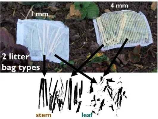
Figure B.1: Litter bag types used for the decomposition study. Litter bags (18 cm x 18 cm) were constructed in accordance with Finerty et al. [7], containing two mesh sizes of 1 mm and 4 mm, to evaluate the contribution of macrofauna decomposition. A fine mesh (1 mm) was used on the bottom for both litter bags to avoid loss of litter material. In addition, two types of litter sources were used to see effects of soil fauna on contrasting litter traits. Oven dried (40°C) leaf and stem material of Zea mays (only top 30 cm of the plant leaves) were used as litter materials. An amount of 2 ± 0.01 g of each leaf and stem pieces (16 ± 1 cm length) have been placed into the litter bags.
1 2 3 4 −2 −1 0 1 2 fitted(mod) resid(mod) Tukey−Anscombe Plot −2 −1 0 1 2 −2 −1 0 1 2
Normal qq−plot, residuals
Theoretical Quantiles Sample Quantiles 1 2 3 4 0.2 0.4 0.6 0.8 1.0 1.2 1.4 fitted(mod) sqr t(abs(resid(mod))) −2 −1 0 1 2 −1.5 −1.0 −0.5 0.0 0.5 1.0
Normal qq−plot, random effects
Theoretical Quantiles
Sample Quantiles
40 60 80 100 −40 −20 0 20 fitted(mod) resid(mod) Tukey−Anscombe Plot −2 −1 0 1 2 −40 −20 0 20
Normal qq−plot, residuals
Theoretical Quantiles Sample Quantiles 40 60 80 100 1 2 3 4 5 6 7 fitted(mod) sqr t(abs(resid(mod))) −2 −1 0 1 2 −20 −10 0 10
Normal qq−plot, random effects
Theoretical Quantiles
Sample Quantiles
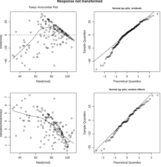
Response not transformed
Figure B.2: Diagnostic residual and random effect plots for the assessment of model assumptions. Transformed model: lmer(log(100−response+1) ∼ MS IR+ S + EShannon+ PS V + T ED + urban warming + land − use types + garden types + (1|Garden ID), REML = F). Upper left: residuals versus fitted values. Upper right: Normal QQ plot of the residuals. Lower left: square-root of the absolute values of the residuals versus fitted values. Lower right: Normal QQ plot of the random effects.
Trochulus clandestin us Trochulus ser iceus Monachoides incar natust Hygromia cinctella Cepaea nemor alis Cepaea hor tensis Helix pomatia Fr uticicola fr uticum Limax maxim us Boettger illa pallenst Derocer as Punctum p ygmaeum P ar alaoma ser vilist Discus rotundatus Ar ion Tandonia b udapestensis Oxychilus cellar iust Oxychilus dr apar naudi Aegopinella minor t Aegopinella pur at Aegopinella nitenst Neso vitrea hammonis Columella edentula Vertigo pusillat Vertigo antiv ertigo Vertigo pygmaeat Vallonia excentrica Vallonia pulchella Vallonia costata Pupilla m uscor um Cochlicopa lubr ica Cecilioides aciculat Vitrea cr ystallina Vitrea contr actat Vitr inobr achium bre v et Succinea putr ist Succineab longat Laciniar ia plicata Macrogastr a atten uata Car ychium tr identatumt Galba tr uncatula Acicula lineatat Lepidocyr tus violaceus Lepidocyr tus cy aneust Lepidocyr tus lignor um Pseudosinella albat Pseudosinella pseudopettersenit Entomobr ya m ultif asciatat Entomobr ya marginatat Heterom ur us nitidus Desor ia Par isotoma notabilis Isotom urus balteatust Isotom urus gr aminist Isotomur us palustr is Isotomiella minor t Isotoma vir idis Folsomia similist Folsomia candida Folsomia spinosat Folsomia quadr ioculata Cr yptop ygus ther mophilust Folsomides par vulust P ogonognathellus fla vescens Hypogastr ur a pur purescens Cer atoph ysella bengtssonit Cer atoph ysella denticulata Schoettella un unguiculata Choreutin ula iner mist Nean ura m uscor um Kalaphor ura Protaphor ur a pulvinatat On ychiur us Stenaphor ura denisit Metaphor ura affinist T ullbergia macrochaetat Megalothor ax minim us Sminthur inus aureust Sphaer idia pumilis Bour letiella hor tensis Dicyr tominar nata Lumbr icus castaneust Lumbr icus r ubellus Lumbr icus terrestr is Lumbr icus f estivus Octolasion cyaneum Octolasion lacteum Dendrodr ilus rubidust Dendrodr ilus subr ubicundust Allolobophora chlorotica Dendrobaenactaedra Aporrectodea icter ica Aporrectodea giardi Aporrectodea longa Aporrectodea roseat Aporrectodea tuberculata Aporrectodea noctur na Aporrectodea caliginosa Ligidium hypnorum Oniscus asellus Philoscia muscorum Trachelipus r athkiit Hyloniscus r iparius Androniscus roseust Haplophthalm us danicus Haplophthalm us mengei Trichoniscus p ygmaeus Cylisticus con vexus Armadillidium v ersicolor t Armadillidium nasatum Armadillidium vulgare Platyarthr us hoffmannseggii Porcellionides pr uinosus Porcellio scaber
Figure B.3: Phylogenetic tree of decomposer organisms based on the open tree of life project [9]. Pictures symbolise the four broad taxonomic groups: collembola (39 species), isopods (16 species), gastropods (42 species) and earthworms (18 species), representing the decomposer fauna in this investigation.
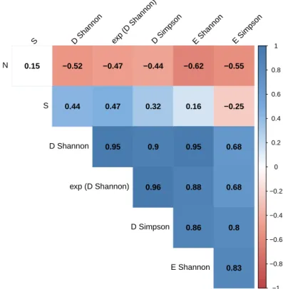
−1 −0.8 −0.6 −0.4 −0.2 0 0.2 0.4 0.6 0.8 1
S D Shannon exp (D Shannon)D Simpson E Shannon E Simpson
N S D Shannon exp (D Shannon) D Simpson E Shannon 0.15 −0.52 0.44 −0.47 0.47 0.95 −0.44 0.32 0.9 0.96 −0.62 0.16 0.95 0.88 0.86 −0.55 −0.25 0.68 0.68 0.8 0.83
Figure B.4: Pearson’s correlation coefficient matrix of taxonomic diversity indices. Non-significant correlations are left blank (P<0.05) calculated with a modified version of the ’corrplot’ package [22]. Species richness (S) and Shannon evenness (E Shannon) were selected to represent species richness and evenness in this study.
−1 −0.8 −0.6 −0.4 −0.2 0 0.2 0.4 0.6 0.8 1
evenness TOP TED FDis PSV PSE PSR PD
species richness evenness TOP TED FDis PSV PSE PSR 0.16 0.73 0.2 0.08 −0.03 0.25 0.15 0.75 0.29 0.06 0.03 0.33 0.13 −0.03 0.21 0.13 0.73 0.24 0.11 0.72 0.32 0.88 0.16 0.73 0.17 0.13 0.17 0.19 0.8 0.07 0.66 0.2 0.04 0.2 0.14 0.9
Figure B.5: Pearson’s correlation coefficient matrix of taxonomic (species richness and evenness), functional (TOP, TED and FDis) and phylogenetic (PSV, PSE, PSR and PD) diversity indices. Trait even distribution (TED) and phylogenetic species variability (PSV) were selected together with species richness and evenness, due to the lowest correlation coefficient in order to avoid collinearity issues [4]. Non-significant correlations are left blank (P<0.05).
−1 −0.8 −0.6 −0.4 −0.2 0 0.2 0.4 0.6 0.8 1
w
ater
management inde
x
fer
tiliz
er
pesticides disturbancew
eeding
removing leaves
water
management index
fertilizer
pesticides
disturbance
0.47
0.45
0.56
0.18
0.38
0.46
0.42
0.32
0.52
0.51
0.26
0.4
0.54
0.34
0.28
−0.1
0.23
0.34
0.36
0.28
0.33
Figure B.6: Pearson’s correlation coefficient matrix of garden management variables. All management questions can be seen in Table A.6. Management variables has been asked individually per land-use type. Water= frequency of applying water (WaterLawn, WaterVeg, Wa-terFlower), management index= sum of all management variables ordered from low to high intensity each on a five level Likert scale, fertiliser= frequency of applying fertiliser (FertLawn, FertGrass, FertVeg, FertFlower), pesticides = frequency of applying pesticides (Pest-Lawn,PestVeg,PestFlower,PestTrees,WeedingHerbicide), disturbance= frequency of soil disturbances (DiggingVeg, DiggingFlower, CareLawn), weeding= frequency of weeding (Weeds). Non-significant correlations are left blank (P<0.05).
−1
−0.8
−0.6
−0.4
−0.2
0
0.2
0.4
0.6
0.8
1
sealed area 30 m
sealed area 50 m
sealed area 100 m
sealed area 250 m
sealed area 500 m
urban warming
sealed area 30 m
sealed area 50 m
sealed area 100 m
sealed area 250 m
0.72
0.76
0.98
0.83
0.9
0.95
0.86
0.8
0.85
0.93
0.86
0.74
0.78
0.86
0.93
Figure B.7: Pearson’s correlation coefficient matrix of urban warming and sealed area. Urban warming is a measure of the local deviation of average night temperatures near surface in the city of Zurich. It is derived from a regional climate model by Parlow et al. [16] and consists of six categories from 0 to+ 6 °C. The sealed areas are the sum of sealed and built area around each garden with five radii (30, 50, 100, 250, 500 m) obtained in ArcGIS.
● ● ● ● ● ● ● ● ● ● ● ● ● ● ● ● ● ●
Urban warming
Garden types: home
Land−use types: grass
Land−use types: forbs
MSIR
PSV
TED
E
Shannon
S
−0.5 0.0 0.5 1.0Fixed effect coefficients
● ●Leaf 1mm
Stem 1mm
Figure B.8: Litter decomposition model fixed effect plots with 1 mm mesh size. Points indicate mean values of simulated Bayesian inference posterior distribution with the 95 % credible intervals as lines. Colours correspond to litter types.
0 25 50 75 100 60 80 100 120 MSIR Leaf 4mm decomposition [%] 0 25 50 75 100 10 15 20 25 30 S 0 25 50 75 100 0.25 0.50 0.75 E_Shannon 0 25 50 75 100 0.4 0.5 0.6 0.7 PSV 0 25 50 75 100 0.85 0.90 0.95 TED Leaf 4mm decomposition [%] 0 25 50 75 100 0 1 2 3 4 5 UHI effect ● 0 25 50 75 100
crops forbs grass
● 0 25 50 75 100 allotment home 0 20 40 60 80 100 120 MSIR Stem 4mm decomposition [%] 0 20 40 10 15 20 25 30 S 0 20 40 0.25 0.50 0.75 E_Shannon 0 20 40 0.4 0.5 0.6 0.7 PSV 0 20 40 0.85 0.90 0.95 TED Stem 4mm decomposition [%] 0 20 40 0 1 2 3 4 5 UHI effect ● 0 20 40
crops forbs grass
●
0 20 40
allotment home
Figure B.9: Effect plots of litter decomposition model showing the fixed effects microbial activity (MSIR), soil fauna species richness (S), species evenness (E Shannon), phylogenetic species variability (PSV), trait even distribution (TED), urban warming, garden land-use types and garden types. Solid lines or bold points are fitted values of the simulated Bayesian inference posterior distribution taking into account the random effect of garden identity with the 95% credible intervals as dotted lines.
● ● ● ●● ● ● ● ● ● ● ● ●● ● 0.0 0.5 1.0 1.5 0 1 2 3 4 5 Distance [km] Semiv ar iance A ● ● ● ● ● ● ● ● ● ● ● ● ● ● ● 0.0 0.5 1.0 1.5 0 1 2 3 4 5 Distance [km] Semiv ar iance B ● ● ● ● ●● ● ● ● ● ● ●● ● ● 0.0 0.5 1.0 1.5 0 1 2 3 4 5 Distance [km] Semiv ar iance C
Figure B.10: Semivariograms of LMEM residuals from the response variables of the decomposition model: leaf 4 mm (A), the model with the microbial activity: MSIR (B) and the model with plant species richness (C). Semivariances (0.5 times the mean squared differences between sites) were computed with the R package ‘gstat’ [17]. In all plots values are close to 1 and show no clear increase or decrease patterns of spatial autocorrelation, indicating that the residuals are not more similar or dissimilar to each other than expected by chance [11]. In addition, the calculated Moran’s I autocorrelation index [15] for the response variable leaf 4 mm was not significant (p=0.26; observed=-0.01±0.004, expected=-0.007) as well as for the response variable MSIR (p=0.09; observed=-0.013±0.004, expected=-0.007) and the response variable plant species richness (p=0.65; observed=-0.008±0.004, expected=-0.007). ● ● ● ● ● ● ● ● ● ● ● ● ● ● ● ● ● ● ● ● ● ● ● ● ● ● ● ● ● ● ● ● ● ● ● ● ● ● ● ● ● ● ● ● ● ● ● ● ● ● ● ● ● ● ● ● ● ● ● ● ● ● ● ● ● ● ● ● ● ● ● ● ● ● ● ● ● ● ● ● ● ● ● ● ● ● ● ● ● ● ● ● ● ● ● ● ● ● ● ● ● ● ● ● ● ● ● ● ● ● ● ● ● ● ● ● ● ● ● ● ● ● ● ● ● ● ● ● ● ● ● ● ● ● ● ● ● ● ● ● ● ● ● ● ● ● ● ● ● ● ● 10 20 30 40 50 Crops (N=41) Forbs (N=48) Grass (N=62) Plant species r ichness
Figure B.11: Plant species richness per garden land-use type assessed as the sum of all cultivated and spontaneously growing plants per urban garden study site. Sampling and methodology of identification including the complete species list can be found in [8]. Bold points represent mean values of the simulated Bayesian inference posterior distribution [11] of the LMEM with garden ID as random factor and garden land-use types as fixed effects. Lines indicate 95 % credible intervals. Estimated LMEM coefficients of fixed effects can be found in Table A.10.
0.5 1.0 1.5 2.0 2.5 3.0 3.5 −2 −1 0 1 2 Tukey−Anscombe Plot Fitted values Residuals −2 −1 0 1 2 −2 −1 0 1 2 Normal QQ−plot Residuals Theoretical Quantiles Sample Quantiles −2 −1 0 1 2 −0.4 −0.2 0.0 0.2 0.4 Normal QQ−plot Random effects Theoretical Quantiles Sample Quantiles
SEM: litter decomposition
−1.5 −1.0 −0.5 0.0 0.5 1.0 1.5 2.0 −2 −1 0 1 2 Tukey−Anscombe Plot Fitted values Residuals −2 −1 0 1 2 −2 −1 0 1 2 Normal QQ−plot Residuals Theoretical Quantiles Sample Quantiles −2 −1 0 1 2 −0.10 −0.05 0.00 0.05 0.10 0.15 Normal QQ−plot Random effects Theoretical Quantiles Sample Quantiles SEM: MSIR −1.5 −1.0 −0.5 0.0 0.5 1.0 1.5 −2 −1 0 1 Tukey−Anscombe Plot Fitted values Residuals −2 −1 0 1 2 −2 −1 0 1 Normal QQ−plot Residuals Theoretical Quantiles Sample Quantiles −2 −1 0 1 2 −0.6 −0.4 −0.2 0.0 0.2 0.4 0.6 Normal QQ−plot Random effects Theoretical Quantiles Sample Quantiles
SEM: Plant species richness
Figure B.12: Residual plots for assessing model assumptions of the LMEM used in the SEM framework. Response variables for the LMEM with leaf 4 mm, microbial activity (MSIR) and plant species richness are plotted (see Table 4 for complete model compositions). Residuals have to be independent and identically distributed, hence they should scatter around zero in the Tukey-Anscombe plots [11]. A few measurements do not fit well to the model as recognisable in the QQ-plots of the residuals, however the majority of the observations seem to fulfil the model assumptions well and since we did not assume a non-linear effect of the assessed variables with the response variables, we accept the slight lack of model assumptions. In addition, we checked the assumptions that the random effects are normally distributed, which was the case in both response values.
60 80 100 120 400 800 1200 1600 Cmic MSIR A 60 80 100 120
0e+00 1e+09 2e+09 3e+09
Bacteria MSIR B 60 80 100 120
0e+00 1e+07 2e+07
Fungi
MSIR
C
Figure B.13: LMEM effect plots of microbial activity (MSIR) as response variable and microbial biomass (Cmic; A), bacterial (B) and fungal (C) qPCR gene copy numbers as fixed effects. Sampling and methodology of bacterial and fungal gene copy numbers can be found in [19]. Lines indicate fitted values of the simulated Bayesian inference posterior distribution [11] of the LMEM with garden ID as random factor. Dotted lines indicate 95 % credible intervals. Estimated LMEM coefficients of fixed effects can be found in Table A.10.
6.5 7.0 7.5 0 1 2 3 4 5 Urban warming pH
A
● ● ● ● ● ● ● ● ● ● ● ● ● ● ● ● ● ● ● ● ● ● ● ● ● ● ● ● ● ● ● ● ● ● ● ● ● ● ● ● ● ● ● ● ● ● ● ● ● ● ● ● ● ● ● ● ● ● ● ● ● ● ● ● ● ● ● ● ● ● ● ● ● ● ● ● ● ● ● ● ● ● ● ● ● ● ● ● ● ● ● ● ● ● ● ● ● ● ● ● ● ● ● ● ● ● ● ● ● ● ● ● ● ● ● ● ● ● ● ● ● ● ● ● ● ● ● ● ● ● ● ● ● ● ● ● ● ● ● ● ● ● ● 6.5 7.0 7.5 Crops (N=38) Forbs (N=46) Grass (N=59) pHB
Figure B.14: LMEM effect plots of soil pH as response variable and urban warming A) and urban garden land-use types B) as fixed effects. Solid line and bold points represent fitted or mean values of the simulated Bayesian inference posterior distribution [11] of the LMEM with garden ID as random factor. Dotted lines and error bars indicate 95 % credible intervals. Estimated LMEM coefficients of fixed effects can be found in Table A.10.
References
[1] Bieri, M., Delucchi, V., and Lienhard, C. (1978). Ein abge¨anderter MacFadyen-Apparat f¨ur die dynamische Extraktion von Bodenarthropoden. Entomologica Germanica, 51:119–132.
[2] Blakemore, R. (2008). An Updated List of Valid, Invalid and Synonym Names of Criodrioidea (Criodrilidae) and Lumbricoidea (Annelida: Oligochaeta: Spar- ganophilidae, Ailoscolecidae, Hormogastridae, Lumbricidae, and Luto- drilidae). PhD thesis, Yokohama National University. [3] Campbell, C. D., Chapman, S. J., Cameron, C. M., Davidson, M. S., and Potts, J. M. (2003). A rapid microtiter plate method to measure carbon dioxide evolved from carbon substrate amendments so as to determine the physiological profiles of soil microbial communities by using whole soil. Applied and environmental microbiology, 69(6):3593–3599.
[4] Dormann, C. F., Elith, J., Bacher, S., Buchmann, C., Carl, G., Carr´e, G., Marqu´ez, J. R. G., Gruber, B., Lafourcade, B., Leit˜ao, P. J., M¨unkem¨uller, T., McClean, C., Osborne, P. E., Reineking, B., Schr¨oder, B., Skidmore, A. K., Zurell, D., and Lautenbach, S. (2013). Collinearity: a review of methods to deal with it and a simulation study evaluating their performance. Ecography, 36(1):27–46.
[5] Ellers, J., Berg, M. P., Dias, A. T., Fontana, S., Ooms, A., and Moretti, M. (2018). Diversity in form and function: Vertical distribution of soil fauna mediates multidimensional trait variation. Journal of Animal Ecology, 87(4):933–944.
[6] Falkner, G., Castella, E., Obrdl´ık, P., and Speight, C. C. D. (2001). Shelled gastropoda of western Europe. Friedrich Held Gesellschaft. [7] Finerty, G. E., de Bello, F., B´ıl´a, K., Berg, M. P., Dias, A. T., Pezzatti, G. B., and Moretti, M. (2016). Exotic or not, leaf trait dissimilarity
modulates the effect of dominant species on mixed litter decomposition. Journal of Ecology, 104(5):1400–1409.
[8] Frey, D., Young, C., Bauer, N., and Moretti, M. (2018). A comprehensive survey of cultivated and spontaneously growing vascular plants in urban gardens. Data in Brief, in press.
[9] Hinchliff, C. E., Smith, S. A., Allman, J. F., Burleigh, J. G., Chaudhary, R., Coghill, L. M., Crandall, K. A., Deng, J., Drew, B. T., Gazis, R., Gude, K., Hibbett, D. S., Katz, L. A., Laughinghouse, H. D., McTavish, E. J., Midford, P. E., Owen, C. L., Ree, R. H., Rees, J. A., Soltis, D. E., Williams, T., and Cranston, K. A. (2015). Synthesis of phylogeny and taxonomy into a comprehensive tree of life. Proceedings of the National Academy of Sciences, 112(41):12764–12769.
[10] Hopkin, S. P. (2007). A key to the Collembola (springtails) of Britain and Ireland. FSC publications, Shrewsbury.
[11] Korner-Nievergelt, F., Roth, T., Von Felten, S., Gu´elat, J., Almasi, B., and Korner-Nievergelt, P. (2015). Bayesian data analysis in ecology using linear models with R, BUGS, and Stan. Academic Press.
[12] Macfadyen, A. (1953). Notes on Methods for the Extraction of Small Soil Arthropods. Journal of Animal Ecology, 22(1):65–77. [13] Macfadyen, A. (1961). Improved Funnel-Type Extractors for Soil Arthropods. Journal of An, 30(1):171–184.
[14] Nakagawa, S. and Schielzeth, H. (2013). A general and simple method for obtaining R2 from generalized linear mixed-effects models. Methods in Ecology and Evolution, 4(2):133–142.
[15] Paradis, E. (2018). Moran’s autocorrelation coefficient in comparative methods. Technical report.
[16] Parlow, E., Scherer, D., and Fehrenbach, U. (2010). Klimaanalyse der Stadt Z¨urich (KLAZ) - Wissenschaftlicher Bericht. Technical report. [17] Pebesma, E. J. (2004). Multivariable geostatistics in S: the gstat package. Computers& Geosciences, 30(7):683–691.
[18] Tresch, S., Moretti, M., Le Bayon, R.-C., M¨ader, P., Zanetta, A., Frey, D., and Fliessbach, A. (2018a). A Gardener’s Influence on Urban Soil Quality. Frontiers in Environmental Science, 6(MAY).
[19] Tresch, S., Moretti, M., Le Bayon, R.-C., M¨ader, P., Zanetta, A., Frey, D., Stehle, B., Kuhn, A., Munyangabe, A., and Fliessbach, A. (2018b). Urban Soil Quality Assessment—A Comprehensive Case Study Dataset of Urban Garden Soils. Frontiers in Environmental Science, 6(November):1–5.
[20] Vandel, A. (1960). Isopodes Terrestres. Part 1 Faune de France 64. Lechevalier, Paris.
[21] Watanabe, S. (2010). Asymptotic equivalence of Bayes cross validation and widely applicable information criterion in singular learning theory. Journal of Machine Learning Research, 11(Dec):3571–3594.
![Table A.3: 19 substrates used for the assessment of the Community level physiological profile (CLPP) based on the MicroResp™ technique [3].](https://thumb-eu.123doks.com/thumbv2/123doknet/14822038.616024/3.892.310.583.358.699/table-substrates-assessment-community-physiological-profile-microresp-technique.webp)
![Table A.7: Model selection based on goodness of fit statistics for LMEM, the widely applicable information criterion (WAIC), a Bayesian version of the AIC [21] and explained variance of the fixed e ff ects R 2 Marginal and including the random e ff ect and](https://thumb-eu.123doks.com/thumbv2/123doknet/14822038.616024/9.892.243.649.326.686/selection-statistics-applicable-information-criterion-bayesian-explained-marginal.webp)
![Figure B.3: Phylogenetic tree of decomposer organisms based on the open tree of life project [9]](https://thumb-eu.123doks.com/thumbv2/123doknet/14822038.616024/17.892.193.697.331.843/figure-phylogenetic-tree-decomposer-organisms-based-open-project.webp)