HAL Id: hal-00501845
https://hal.archives-ouvertes.fr/hal-00501845
Submitted on 12 Jul 2010
HAL is a multi-disciplinary open access
archive for the deposit and dissemination of
sci-entific research documents, whether they are
pub-lished or not. The documents may come from
teaching and research institutions in France or
abroad, or from public or private research centers.
L’archive ouverte pluridisciplinaire HAL, est
destinée au dépôt et à la diffusion de documents
scientifiques de niveau recherche, publiés ou non,
émanant des établissements d’enseignement et de
recherche français ou étrangers, des laboratoires
publics ou privés.
Multiway Space-Time-Wave-Vector Analysis for Source
Localization and Extraction
Hanna Becker, Pierre Comon, Laurent Albera, Martin Haardt, Isabelle Merlet
To cite this version:
Hanna Becker, Pierre Comon, Laurent Albera, Martin Haardt, Isabelle Merlet. Multiway
Space-Time-Wave-Vector Analysis for Source Localization and Extraction. European Signal Processing Conference,
Aug 2010, Aalborg, Denmark. pp.1349-1353. �hal-00501845�
MULTIWAY SPACE-TIME-WAVE-VECTOR ANALYSIS
FOR SOURCE LOCALIZATION AND EXTRACTION
Hanna Becker
1,2, Pierre Comon
1, Laurent Albera
3, Martin Haardt
2, Isabelle Merlet
3 (1) Lab. I3S, UMR6070 CNRS,Univ. of Nice, BP 121, F-06903 Sophia-Antipolis, France
tel: + 33 492942717, fax: +33 492942898 [email protected], [email protected]
(2) Comm.Research Lab., Ilmenau Univ. of Technology, PO Box 100565,
D-98684 Ilmenau, Germany
tel: +49 3677692613, fax: +49 3677691195 [email protected]
(3) Inserm, UMR 642, LTSI, Bat. 22, Univ. Rennes 1, F-35042 Rennes
Cedex, France
tel: +33 223235058, fax: +33 223236917, [email protected]
ABSTRACT
Deterministic approaches for source localization and extrac-tion are desirable for short or nonstaextrac-tionary data, as op-posed to techniques based on second or higher order statis-tics. Techniques based on tensor decompositions are recog-nized to be efficient in this framework, provided some di-versity is available, in addition to time and space. With this goal, some authors have proposed to decompose a Space-Time-Frequency data tensor. In this paper, we propose a new multiway approach based on Space-Time-Wave-Vector (STWV) data which is obtained by a 3D local Fourier trans-form over space accomplished on the measured data. This method does not only permit to accurately localize sources even in a noisy environment, but simultaneously extracts the temporal behaviour associated with each source. The per-formance of this STWV analysis is investigated by means of computer simulations in the context of
ElectroEncephalo-Graphic (EEG) data analysis.1
1. INTRODUCTION
Most antenna array processing techniques are devoted to the localization of radiating sources. When signal copies are re-quired, another procedure needs to be executed after localiza-tion. This two-stage approach has several drawbacks. First, the signal estimation quality depends on the accuracy of the localization stage. Second, when the knowledge of the array manifold is utilized, the estimation of sources is sensitive to calibration errors. Third, properties of the sources (such as nonstationarity, sparseness...) are not utilized. And fourth, techniques based on second or higher order statistics are not robust in case of very short data records.
With this in mind, deterministic techniques based on tensor CANonical Decompositions (CAND) – sometimes known as PARAFAC – have been introduced; see, e.g., [1]. The common feature of these techniques is that an additional diversity is required, and that the array manifold is not used, at least in a first stage. In order to restore identifiability, a proper tensor of order strictly greater than two is built, by exploiting this diversity. In [1] for instance, this diversity comes from a space invariance of the array of sensors.
Several authors have studied the use of the CAND ap-plied to Space-Time-Frequency (STF) data [3, 4, 5, 6, 7].
1This work has been supported in part by ANR-06-BLAN-0074 project
Decotes, and the Computational Advances in Multi-Sensor Signal Process-ing (CAMUS) DFG project.
The method was tested both on real and simulated data and led to promising results. However, this technique has some limitations pointed out in Section 3.
In the following, we present a different multiway-approach, which is extraneous to the temporal behaviour of the sources. Our technique is based on data transformed into the Space-Time-Wave-Vector (STWV) domain. The advan-tage of this method is that it permits to accurately localize one or several dipole sources and extract at the same time a good estimate of the associated source signals. Moreover, it is very robust to additive white Gaussian noise.
2. MULTILINEAR MODELING
Data are collected with the help of an array of sensors as a function of time and at various locations. Hence this
bivari-ate function x(r,t), sampled in time and space, can be stored
in a data matrix X∈ RN×Kwhere N and K denote the
num-ber of sensors and time samples, respectively. Assuming a static propagation medium, this matrix can be factorized into
a mixing matrix Ao∈ RN×R, depending on spatial
parame-ters and a signal matrix S∈ RR×K, which contains the time
samples of the R sources:
X= AoS (1)
The goal is to find a relevant transformation allowing to pro-duce a data tensor from the matrix X. In fact, in contrast to matrices, a tensor of order strictly greater than two admits a unique decomposition into a sum of rank-one terms, under a reasonable assumption on its rank (see below). This allows to restore identifiability in a number of problems.
Notation. Once bases of the linear spaces are fixed, ten-sors of order d are represented by d-way arrays. For sim-plicity, they are then usually identified with their array repre-sentation. We assume the following notation throughout this paper: bold italic uppercase letters denote tensors, e.g. , T, bold uppercase letters denote matrices, e.g. , A, bold low-ercase letters denote column vectors, e.g. , a, and plain font
denotes scalars, e.g. , Xi jk, Ti jor ai.
CAND decomposition. Let T be a third order tensor of
dimensions I×J×K. The rank of T is defined as the minimal
number P of vector outer products that need to be summed up in order to have the exact representation below:
Ti jk= P
∑
p=1
When P is smaller than the bound I+J+K−2IJK , the above
de-composition into decomposable tensors2 is almost surely
unique (see, e.g. , [2] and references therein), and will be
referred to as Canonical, and denoted with the CAND3
acronym. Note that, even when the CAND of T is unique, it is non uniquely represented by 3 loading matrices A, B and
C of size I×P, J×P and K ×P, respectively. In fact, scale
and permutation indeterminacies (which may be fixed) exist in such a representation.
2.1 Space-Time-Frequency (STF) analysis
In order to collect an additional diversity to turn the data ma-trix X into a tensor, a frequently used idea is to compute the wavelet transform (or a short-term Fourier transform) of the measured data. If we assume that time and frequency variables approximately separate in the time-frequency trans-form of every source signal, which means that the frequency content of each signal has to be approximately constant over time, then the bilinear model (1) is transformed to a trilinear one. In other words, one obtains a 3rd order tensor W, which admits the CAND below:
W(r,t, f ) =
P
∑
p=1
a(r; p) b(t; p) c( f ; p) (2) In fact, the variables r, t and f (denoting the sensor loca-tion, the time index and the frequency index, respectively) are sampled and hence belong to finite sets, so that the di-mensions of W are finite and the above decomposition is in-deed a CAND. Note that the exact functional decomposition (2) into a finite sum of functions with separated (continuous) variables does not exist in general.
2.2 Space-Time-Wave-Vector (STWV) analysis
Instead of applying a transform on the time variable, one can instead act on the space variable. If a 3D Fourier transform is computed within a small patch on the sensor array, which is selected by the window function w centered at r, the trivariate function below is obtained, where the third dimension is now the wave vector k.
F(r,t, k) =
Z ∞
−∞w(r
′− r) x(r′,t)ejkTr′
dr′ (3)
Similarly to the STF approach, a CAND decomposition into a finite number of components P is possible.
F(r,t, k) =
P
∑
p=1
a(r; p) b(t; p) c(k; p) (4) The number of terms, P, equals the number of dipolar sources if the wave vector content of each of the components is the same at every sensor.
2.3 Source extraction
After separating the measured data into several components associated with different sources using the CAND model, an
2decomposable tensors are by definition rank-1 tensors [8].
3One could also talk about “polyadic decompositions”; see [9] and
ref-erences therein.
estimate of the time samples of theses sources can be readily obtained. The STWV analysis is particularly well suited for this purpose because the temporal characteristics extracted by the CAND of the tensor F constitute an accurate
approx-imation ˆS of the signal matrix S. This property is due to the
fact that the Fourier transform over space does not affect the source activities, which means that the tensor F admits the exact bilinear model:
F(r,t, k) =
P
∑
p=1
b(t; p) D(r, k; p) (5) By contrast, to estimate the signal activities using the STF analysis, the signal matrix needs to be computed using the pseudo-inverse of the mixing matrix. This can be
prob-lematic if Aois not a tall matrix, meaning that there are more
sources than sensors. 2.4 Source localization
Another reason for using tensor modeling and CAND de-compositions is that an estimate of the source positions can be determined. The source localization consists of two steps, the estimation of the mixing matrix and the determination of the source parameters which best match the estimated mixing matrix using a non-linear least squares algorithm.
In the case of the STF method, the wavelet transform does not affect the mixing matrix, which means that the spa-tial characteristics A extracted with the STF approach al-ready constitute a good approximation for the mixing matrix
Ao.
The STWV approach however, via its Fourier transform over space, does not lead to clearly separated space and wave vector characteristics. Consequently, the loading matrix A of the STWV method does not permit to localize the source, and another approach based on the signal matrix has to be taken.
Once an accurate estimate ˆS of the signal matrix is available
(see previous section), the mixing matrix can be computed from:
ˆ
Ao= X ˆS+ (6) using the original data. Note that, since it is always possible to have more time samples than sources, the computation of
the pseudo-inverse ˆS+of the signal matrix ˆS does not raise
any problem.
3. EEG APPLICATION
One possible application for multiway models is the analysis of ElectroEncephaloGraphic (EEG) data, on which we focus in this article. Due to its good temporal resolution compared to other methods (like for example functional Magnetic Res-onance Imaging (f-MRI)), EEG is routinely used to record seizures in epileptic patients. An important issue in this re-gard is the identification of the epileptogenic zone, which can then be removed by surgery. To localize the sources underly-ing the electric potential measured on the surface of the scalp a multitude of different approaches has been proposed in the past [10]. These methods vary mainly in the assumptions made on the nature and the number of sources. A common technique consists in fitting a few equivalent dipolar sources to the measured EEG data. The performance depends es-sentially on the assumptions which are exploited to localize
these sources and on the parameters related to the method applied. The statistical approach described in [11] is there-fore limited by the number of time samples used to estimate higher order statistics, and its performance depends on the statistical properties of source signals. In [12, 13] an analyt-ical approach is presented for the localization of monopole and dipole sources within a disk from given boundary data.
In [3, 4, 5, 6, 7], the CAND is applied to STF EEG data. But this technique does not permit to separate several simul-taneously active brain regions with correlated activities into more than one component, thus preventing the representa-tion of such a scenario by an adequate number of equivalent dipoles.
4. COMPUTER RESULTS
In this section, we focus on the application of the STF and STWV analyses to EEG data and investigate the influence of various parameters on the capability of localizing superficial, radially oriented dipole sources with the help of computer simulations. To this end, electric potential data are gener-ated using a 3-shell spherical head model (cf. [11, 14]) to construct the mixing matrix, which is in this context also called the leadfield matrix, and describes the geometry and conductive properties of the head; then white Gaussian noise is added (this corresponds to preprocessed noisy EEG data, where artifacts have already been removed). The radii of the shells representing brain, skull and scalp are 8 cm, 8.5
cm and 9.2 cm with conductivities 3.3 × 10⁻³, 8.25 × 10⁻⁵
and 3.3 × 10⁻³. The Jansen model [15] is used to create
K= 200 snapshots of epileptic activity at time intervals of T = 0.008 s. To construct the tensor W ∈ RN×K×M where
M= K stands for the number of frequency snapshots in the
STF approach, the discrete Wavelet transform is used with a
real-valued Morlet-Wavelet. The tensor F∈ CN×K×J is
ob-tained using the non-uniform, discrete 3D local Fourier trans-form over space with a Blackman window function where
J= 63 is the number of wave vectors.
A rank P approximate of each of the data tensors is then determined with a semi-algebraic CAND, namely a Joint Ap-proximate Diagonalization (JAD) algorithm [16], followed – in the case of the STWV method, where the tensor F is com-plex – by one step of the alternating least squares algorithm to ensure a real valued loading matrix B for the discrete-time signals. The optimal rank P is determined using Corcon-dia [17]. In the case of the STWV analysis, the number of components P extracted from F can be assumed to equal the number of dipolar sources R because the hypothesis that the wave vector content of each of the components is the same at every sensor is reasonably well met for superficial dipolar sources as examined here. This is due to the fact that the en-ergy at each source is concentrated within a small region on the scalp where the wave vector content is nearly identical. On the contrary, for the STF approach, R generally equals
P− 1 in the presence of noise because noise accounts for an
additional component [3, 4] in (2).
Eventually, the source extraction is analyzed by the correlation between original source time signals and esti-mated temporal characteristics as an intermediate result in the source localization process of the STWV technique. Fi-nally, the source locations are estimated according to the STF
and STWV methods described above, and the RMSE local-ization error is computed according to
RMSE= v u u t 1 R R
∑
p=1 ||ˆrqp− rqp||2 (7)where ˆrqp and rqpdenote the estimated and original source
positions, respectively.
Number of time samples. To examine the influence of the number of time samples on the performance of the mul-tiway methods, the correlation coefficient between estimated and original signals, and the RMSE localization error of a
source positioned at rq= [−π/12,π/5, 8] (in spherical
coor-dinates) are determined for different numbers of time sam-ples; see Figure 1. The EEG data are recorded at a SNR of -3 dB using 64 electrodes. The results consist of the outcome of 200 trials and show that the STWV analysis allows for an accurate source extraction, which diminishes only for less than 40 time samples. Furthermore, the STWV method still permits to localize the dipole source if only very few tempo-ral snapshots are used whereas more than 150 time samples are necessary for the STF analysis to give nearly as accurate results. If the tensors of both approaches are of the same
size (which is the case for K= 63 temporal snapshots), the
STWV method clearly leads to better results.
Influence of noise. Since EEG data is usually very noisy, an important issue of source localization methods is their robustness to noise. In the following simulation, the influence of additive spatially and temporally white Gaus-sian noise on the source localization accuracy is examined for both STWV and STF analyses. The dipole source is
po-sitioned at rq= [π/2,π/8, 8] (in spherical coordinates) and
the electric potential X is computed for 64 sensors. To ob-tain noisy data a matrix conob-taining white Gaussian noise is
added according to the SNR Ps/Pn where Pn is the power
of the noise and where the signal power is given by Ps=
1
N·K∑Ni=1∑Kj=1X2i j. Subsequent results, displayed in Figure 2
(top and middle) , constitute an average over at least 200 tri-als with different noise and signal matrices. Even for a SNR of -8 dB, the correlation coefficient between original and es-timated source time signals is more than 90 %, which means that the signal activity is still well captured by the STWV method. This can also be seen in Figure 2 (bottom) where original and estimed signals are plotted for a SNR of -3 dB.
Regarding the source localization, the STWV approach leads to results clearly superior to those of STF analysis. This can be explained by the fact that the STWV method reduces the noise by computing a local average over space at the time of the 3D Fourier transform and averaging over time when the leadfield matrix is calculated from the
pseudo-inverse of the estimated signal matrix ˆS. On the contrary, the
STF method tries to eliminate the noise by separating it into an additional component of the CAND model, which is often not as efficient.
Several sources. If there are several dipole sources of epileptic activity, a main point of interest is whether they can be separated accurately. In the case of the STWV approach, this depends largely on the distance between the sources and the number of sensors used to record the scalp potential.
20 40 60 80 100 120 140 160 180 200 0
0.5 1 1.5
number of time samples
source localization error in cm
STWV approach STF approach 20 40 60 80 100 120 140 160 180 200 0.95 0.955 0.96 0.965 0.97 0.975 0.98 0.985 0.99 0.995 1
number of time samples
correlation coefficient
Figure 1: (Top) RMSE source localization error and (bot-tom) correlation coefficient of original and estimated signals for the STWV approach plotted as a function of the number of time samples for a SNR of -3 dB and 64 electrodes.
In the absence of noise, the STWV method permits for example to distinguish two sources separated by a distance of 3.35 cm up to a RMSE of 0.52 cm if 128 sensors are used. On the contrary, if electric potential data are only available at 32 positions, the sources cannot be separated. This is only possible if the distance is increased to 4 cm, although this leads to a relatively high RMSE of 1.03 cm.
For the STF method, the energy, the frequency and the correlation of the source activities are the crucial fac-tors determining whether a distinction of the sources is
possible. An accurate estimation of the source location
can only be achieved if the characteristics of different sources are not mixed in the components extracted using the CAND decomposition. Resulting problems can for in-stance be seen in a simulation with three sources located at rq1= [−π/2,π/4, 8], rq2 = [−π/12,π/5, 8] and rq3 =
[π/2,π/5, 7] where the STF approach does not allow to
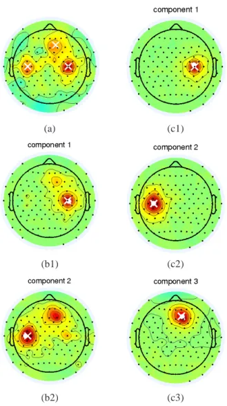
sep-arate all sources because of their similar activities. This be-comes manifest by an optimal tensor rank (determinded by Corcondia) of only two. Since the sources are spread over the whole head, a separation with the help of the STWV method is not hindered though (cf. Figure 3).
−8 −6 −4 −2 0 2 4 6 8 10 0.9 0.91 0.92 0.93 0.94 0.95 0.96 0.97 0.98 0.99 1 SNR in dB correlation coefficient −80 −6 −4 −2 0 2 4 6 8 10 0.1 0.2 0.3 0.4 0.5 SNR in dB
source localization error in cm
STWV approach STF approach 0 50 100 150 200 −3 −2 −1 0 1 2
index of time snapshot
signal amplitude
estimated signal original signal
Figure 2: (Top) Correlation coefficient of original and esti-mated source time signals for the STWV approach and (mid-dle) RMSE source localization error as a function of the SNR
for K= 200 and N = 64. (Bottom) Original and estimated
signals for the STWV approach for SNR= −3 dB, K = 200,
N= 64
5. CONCLUDING REMARKS
As we have demonstrated here in the context of EEG data, the newly presented multiway model is a powerful tool for source analysis, not only providing an estimate of the source locations, but simultaneously extracting the discrete-time signals associated with each of the sources. Moreover, the STWV approach is more robust than STF to white Gaussian noise, especially for short time samples, which could be used to trace the spatial evolution of sources. Problems are only
(a) (c1)
(b1) (c2)
(b2) (c3)
Figure 3: Topographic plots of the absolute values of the original potential distribution, (a) averaged over all time sam-ples; the estimates for both (b) the STF analysis and (c) the STWV approach for 128 sensors, 200 time samples and a SNR of -3 dB. Original dipole positions are marked by a white cross, estimated dipole locations by a white point.
encountered when trying to separate very close sources, but if the dipolar EEG sources cannot be distinguished because of their small distance despite a sufficient spatial resolution of at least 64 electrodes, they are likely to belong to the same, larger source. The identification of such distributed sources, which constitute a more realistic representation of the under-lying physiological phenomena, is a crucial aspect in EEG analysis and will be addressed in further studies.
REFERENCES
[1] N. D. Sidiropoulos, R. Bro, and G. B. Giannakis, “Par-allel factor analysis in sensor array processing,” IEEE
Trans. Sig. Proc., vol. 48, no. 8, pp. 2377–2388, 2000.
[2] P. Comon, X. Luciani, and A. L. F. De Almeida, “Ten-sor decompositions, alternating least squares and other tales,” Jour. Chemo., vol. 23, pp. 393–405, Aug. 2009.
[3] M. De Vos, A. Vergult, L. De Lathauwer, et al., “Canon-ical decomposition of ictal scalp EEG reliably detects the seizure onset zone,” NeuroImage, vol. 37, pp. 844– 854, 2007.
[4] M. De Vos, L. De Lathauwer, V. Vanrumste, et al., “Canonical decomposition of ictal scalp EEG and ac-curate source localisation: Principles and simulations study,” Comput. Intel. Neurosc., pp. 1–10, Dec. 2007. [5] F. Miwakeichi, E. Martinez-Montes, P. A. Valdes-Sosa,
N. Nishiyama, H. Mizuhara, and Y. Yamaguchi, “De-composing EEG data into space-time-frequency com-ponents using parallel factor analysis,” NeuroImage, vol. 22, pp. 1035–1045, 2004.
[6] M. Weis, F. Roemer, M. Haardt, D. Jannek, and
P. Husar, “Mutli-dimensional space-time-frequency
component analysis of event related EEG data using closed-form PARAFAC,” in ICASSP, Taipei, 2009. [7] M. Morup, L. K. Hansen, C. S. Herrmann, J. Parnas,
and S. M. Arnfred, “Parallel factor analysis as an
exploratory tool for wavelet transformed event-related EEG,” NeuroImage, vol. 29, pp. 938–947, 2006. [8] J. B. Kruskal, “Three-way arrays: Rank and uniqueness
of trilinear decompositions,” Lin. Alg. Appl., vol. 18, pp. 95–138, 1977.
[9] L-H. Lim and P. Comon, “Nonnegative approximations of nonnegative tensors,” Jour. Chemo., vol. 23, pp. 432– 441, Aug. 2009.
[10] R. Grech, T. Cassar, J. Muscat, et al., “Review on solv-ing the inverse problem in EEG source analysis,” J.
NeuroEng. Rehab., vol. 5, Nov. 2008.
[11] L. Albera, A. Ferreol, D. Cosandier-Rimele, I. Merlet, and F. Wendling, “Brain source localization using a fourth-order deflation scheme,” IEEE Trans. Biomed.
Eng., vol. 55, no. 2, Feb. 2008.
[12] L. Baratchart, A. Ben Abda, F. Ben Hassen, and J. Leblond, “Recovery of pointwise sources or small inclusions in 2D domains and rational approximation,”
Inverse Problems, vol. 21, pp. 51–74, 2005.
[13] A. Ben Abda, F. Ben Hassen, J. Leblond, and M. Mahjoub, “Sources recovery from boundary data:
A model related to electroencephalography,” Math.
Comp. Model., vol. 49, pp. 2213–2223, 2009.
[14] J. C. Mosher, R. M. Leahy, and P. S. Lewis, “EEG and MEG: Forward solutions for inverse methods,” IEEE
Trans. Biomed. Eng., vol. 46, no. 3, March 1999.
[15] B. H. Jansen and V. G. Rit, “Electroencephalogram and visual evoked potential generation in a mathematical model of coupled cortical columns,” Biological
Cyber-natics, vol. 73, pp. 357–366, 1995.
[16] F. Roemer and M. Haardt, “A closed-form solution for parallel factor (PARAFAC) analysis,” in ICASSP, Las Vegas, NV, 2008.
[17] R. Bro, Multi-way analysis in the food industry:
Mod-els, algorithms and applications, Ph.D. thesis,
Uni-versity of Amsterdam (NL) and Royal Veterinary and Agricultural University (DK), 1998.