HAL Id: hal-03224056
https://hal.inria.fr/hal-03224056
Submitted on 11 May 2021HAL is a multi-disciplinary open access archive for the deposit and dissemination of sci-entific research documents, whether they are pub-lished or not. The documents may come from teaching and research institutions in France or abroad, or from public or private research centers.
L’archive ouverte pluridisciplinaire HAL, est destinée au dépôt et à la diffusion de documents scientifiques de niveau recherche, publiés ou non, émanant des établissements d’enseignement et de recherche français ou étrangers, des laboratoires publics ou privés.
up the numerical resolution of the 2D shallow water
equations
Joao Guilherme Caldas Steinstraesser, Vincent Guinot, Antoine Rousseau
To cite this version:
Joao Guilherme Caldas Steinstraesser, Vincent Guinot, Antoine Rousseau. Application of a modified parareal method for speeding up the numerical resolution of the 2D shallow water equations. Simhy-dro 2021 - 6th International Conference Models for complex and global water issues - Practices and expectations, Jun 2021, Sophia Antipolis, France. �hal-03224056�
method for speeding up the numerical resolution of the 2D shallow water equations
APPLICATION OF A MODIFIED PARAREAL METHOD FOR SPEEDING
UP THE NUMERICAL RESOLUTION OF THE 2D SHALLOW WATER
EQUATIONS
Joao Guilherme Caldas Steinstraesser1
Inria, IMAG, Univ Montpellier, CNRS, Montpellier, France joao-guilherme.caldas-steinstraesser@inria.fr
Vincent Guinot
Univ Montpellier, HSM, CNRS, IRD, Inria, Montpellier, France vincent.guinot@inria.fr
Antoine Rousseau
Inria, IMAG, Univ Montpellier, CNRS, Montpellier, France antoine.rousseau@inria.fr
KEY WORDS
Shallow water equations, numerical speedup, multiscale simulation, parareal method, reduced-order model
ABSTRACT
In this work, we implement some variations of the parareal method for speeding up the numerical resolution of the two-dimensional nonlinear shallow water equations (SWE). This method aims to reduce the computational time required for a fine and expensive model, by using alongside a less accurate, but much cheaper, coarser one, which allows to parallelize in time the fine simulation. We consider here a variant of the method using reduced-order models and suitable for treating nonlinear hyperbolic problems, being able to reduce stability and convergence issues of the parareal algorithm in its original formulation. We also propose a modification of the ROM-based parareal method consisting in the enrichment of the input data for the model reduction with extra information not requiring any additional computational cost to be obtained. Numerical simulations of the 2D nonlinear SWE with increasing complexity are presented for comparing the configurations of the model reduction techniques and the performance of the parareal variants. Our proposed method presents a more stable behavior and a faster convergence towards the fine, referential solution, providing good approximations with a reduced computational cost. Therefore, it is a promising tool for accelerating the numerical simulation of problems in hydrodynamics.
1. INTRODUCTION
A commonly encountered challenge in the numerical simulation of problems in hydrodynamics is the trade-off between the accuracy of the approximate solution and the computational cost required for computing it. Accurate simulations require fine spatial and temporal discretizations (possibly linked by stability conditions) and/or high-order integration scheme, which may lead to prohibitive computational times and memory demands, thus limiting the practical application of the models.
An alternative for overcoming these difficulties is to use parallel-in-time numerical schemes, of which one of the most popular is the so-called parareal method, an iterative algorithm first developed by [1]. This method, whose objective is to parallelize in time a fine, expensive numerical simulation by using alongside a coarser, cheaper model, stands out for its simple and generic formulation. Indeed, among its various applications, parabolic and diffusive problems are the most successful ones. However, in the case of
method for speeding up the numerical resolution of the 2D shallow water equations hyperbolic and advection-dominated problems, the parareal method presents slow convergence and stability issues [2]. Variants of the method are presented in the literature for reducing these limitations.
In this work, we are interested in using the parareal method for reducing the computational cost for the numerical resolution of the 2D nonlinear shallow water equations (SWE) [3]
∂ℎ ∂𝑡+ ∂(ℎ𝑢') ∂𝑥 + ∂*ℎ𝑢+, ∂𝑦 = 0 (1𝑎) ∂(ℎ𝑢') ∂𝑡 + ∂ ∂𝑥(ℎ𝑢'2+ 𝑔ℎ2/2) + ∂*ℎ𝑢'𝑢+, ∂𝑦 = 0 (1𝑏) ∂(ℎ𝑢') ∂𝑡 + ∂*ℎ𝑢'𝑢+, ∂𝑥 + ∂ ∂𝑦*ℎ𝑢+2+ 𝑔ℎ2/2, = 0 (1𝑐)
where ℎ is the water depth, 𝑢' and 𝑢+ are the flow velocities respectively in the 𝑥- and 𝑦- directions and 𝑔 is
the gravitational acceleration. Usually, the SWE are formulated with source terms accounting for bottom variation and friction dissipation, but these phenomena are neglected here.
Equations (1a)-(1c) are a system of nonlinear hyperbolic equations. Thus, for solving them with the parareal method, we implement a variant proposed by [4] using reduced-order models (ROMs) computed on-the-fly along the parareal iterations. However, even if the ROM-based parareal method is effective for improving the convergence and stability when applied to nonlinear hyperbolic problems, its performance is limited by the quality of the ROMs. Therefore, we propose a modification that consists in enriching the ROMs with extra information whose computation does not require any additional computational cost.
This paper is organized as follows: in Section 2, the original parareal method and its variation using reduced-order models are briefly presented, along with an overview on the model reduction techniques considered here; in section 3, we present our modification to the ROM-based parareal method; in section 4, some numerical tests are presented for studying configurations of the model reduction and comparing the performance of the parareal variants; finally, a conclusion is presented in Section 5.
2. THE PARAREAL METHOD AND ITS VARIATIONS
The parareal method [1], whose name stands for “parallel in real-time", is a predictor-corrector iterative method aiming to reduce the computational cost for the numerical simulation of a fine, expensive model. By using a second, coarser model acting as predictor, the parallel method allows to parallelize the fine simulation in time. However, although its successful application in a variety of problems, mainly parabolic and diffusive ones, the parareal method presents slow convergence and/or instabilities when applied to hyperbolic problems, even the simplest ones as the one-dimensional advection equation [2]. Modifications of the method are presented in the literature for overcoming these difficulties. In the case of nonlinear hyperbolic problems, one of the approaches consists in introducing reduced-order models (ROMs) in the parareal algorithm [4]. We briefly present in this section the original or classical parareal method, following its presentation in [5], and its modification for treating nonlinear hyperbolic problems, called hereafter as
ROM-based parareal method.
2.1 The classical parareal method
We present the parareal method by considering the following nonlinear time-dependent problem 8
𝑑
𝑑𝑡𝒚(𝑡) = 𝐴𝒚(𝑡) + 𝑭(𝒚(𝑡)), in [0, 𝑇]
𝒚(0) = 𝒚B (2)
where 𝒚 ∈ ℝE, 𝐴 is assumed to be time-independent, 𝑭 is a nonlinear function and 𝑇 is the final instant of
simulation. For solving (2) numerically, we define two discretizations (also called propagators) ℱGH and 𝒢JH, associated respectively to homogeneous time steps δ𝑡 and Δ𝑡, with δ𝑡 < Δ𝑡 and Δ𝑡 = 𝑝δ𝑡, where 𝑝 > 1 is an integer (this last assumption is not necessary but considered here for simplification; in a general case, an interpolation procedure between the temporal discretizations would be necessary). We also define the
method for speeding up the numerical resolution of the 2D shallow water equations instants of a discretization of the temporal domain [0, 𝑇] using Δ𝑡 by 𝑡P = 𝑛Δ𝑡, 𝑛 = 0, … , 𝑁JH and 𝑡TUV = 𝑇. These definitions are illustrated in Figure 1.
Figure 1: Definition of the temporal discretization of the fine and the coarse propagators (respectively bullets and
vertical traces). The instants 𝑡P, 𝑛 = 0, … , 𝑁JH correspond to the coarse discretization.
We denote the solution propagated from 𝒚 (defined at 𝑡P) to 𝑡PWX using ℱGH and 𝒢JH respectively by
ℱGH(𝒚, 𝑡PWX, 𝑡P), 𝒢JH(𝒚, 𝑡PWX, 𝑡P)
ℱGH is a fine model (providing an accurate solution compared to analytical and/or experimental ones)
but too expensive in terms of computational time. It is called hereafter as fine propagator and its numerical solution is considered as a referential one. On the other hand, 𝒢JH, called the coarse propagator, has a much
smaller computational cost (generally with δ𝑡 ≪ Δ𝑡), but provides less accurate solutions. We remark that 𝒢JH can also contain other simplifications with respect to ℱGH; for example, a coarser spatial discretization
(which, in the case of hyperbolic problems, is usually defined together with the time step for keeping the same CFL number), lower-order numerical schemes or even simplified equations from the mathematical or physical point of view [6]. However, the only simplification required by the parareal method is the temporal coarsening δ𝑡 < Δ𝑡.
The objective of the parareal method is to provide an accurate numerical solution for (2), with the same or a close accuracy as the fine, referential one, but with a smaller computational cost than the one required for the simulation of ℱGH. This is performed via the following parallel-in-time predictor-corrector procedure:
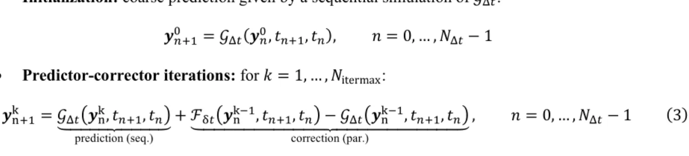
• Initialization: coarse prediction given by a sequential simulation of 𝒢JH: 𝒚PWXB = 𝒢
JH(𝒚PB, 𝑡PWX, 𝑡P), 𝑛 = 0, … , 𝑁JH− 1
• Predictor-corrector iterations: for 𝑘 = 1, … , 𝑁itermax:
𝒚cWXd = 𝒢
JH*𝒚cd, 𝑡PWX, 𝑡P,
effffgffffh
prediction (seq.)
+ ℱeffffffffffffgffffffffffffhGH*𝒚cdiX, 𝑡PWX, 𝑡P, − 𝒢JH*𝒚cdiX, 𝑡PWX, 𝑡P, correction (par.)
, 𝑛 = 0, … , 𝑁JH− 1 (3)
where 𝒚cd is an approximation, in the parareal iteration 𝑘, for the solution of (2) at the instant 𝑡
P of the coarse
temporal discretization; and 𝑁itermax is an user-defined maximum number of parareal iterations. Notice that
the numerical resolution of (3) contains two nested loops: the outer one corresponds to the parareal iterations and, within each iteration, a full time loop (from 0 to 𝑇) is performed, as illustrated in Figure 2.
Figure 2: Schematic representation of the parareal algorithm. A full time loop is performed within each parareal
iteration.
Notice that, for updating the solution in the iteration 𝑘, the correction term of (3), in which the fine propagator is used, depends only on the solution of the previous iteration 𝑘 − 1, already available in the beginning of the iteration for all the instants 𝑡P, 𝑛 = 0, … , 𝑁JH . Therefore, the fine propagations along each
coarse time window [𝑡P, 𝑡PWX] are independent one from another and thus can be parallelized. The only term of (3) that needs to be computed sequentially is the coarse prediction, which has a low computational cost.
method for speeding up the numerical resolution of the 2D shallow water equations Supposing that the parareal simulation is distributed to 𝑁JH parallel processors, then, in each parareal iteration, each processor performs the fine propagation along only one coarse time step. Therefore, in an ideal case, the numerical resolution of ℱGH in each iteration takes 1/𝑁JH of the computational time needed to a full fine, sequential simulation. As an immediate consequence, the parareal method is only interesting if it attains a certain convergence in a small number of iterations, much smaller than the number of coarse time steps 𝑁JH; else, the parareal simulation is more expensive than the referential one. In practice, this fast convergence is verified for several problems, but not for hyperbolic problems, for which stability issues are also observed.
2.2 The ROM-based parareal method
Modifications of the parareal method are proposed in [4] for overcoming the instabilities and slow convergence observed for hyperbolic problems, by using reduced-order models (ROMs) constructed from snapshots of the parareal solution along iterations. In general lines, the objective of the model-order reduction is to reduce the computational complexity of an expensive problem. Suppose that, in problem (2), 𝑀 is very large (for example, the problem is solved in a very refined mesh). Therefore, one may be interested in formulating a simplified reduced problem with a much smaller dimension 𝑞 ≪ 𝑀.
The idea of the ROM-based parareal method is to replace, in each iteration 𝑘 ≥ 1, the coarse propagator 𝒢JH by a ROM ℛGHo , solved with the same small time step δ𝑡 of the fine propagator. Therefore, the
ROM ℛGHo is seen as an unexpensive approximation of ℱ
GH. In the case of nonlinear hyperbolic problems, the
ROMs are formulated using two combined model reduction techniques, used respectively for reducing the linear and the nonlinear term of the equations: the proper orthogonal decomposition (POD) and the empirical interpolation method (EIM) [7]; for this last one, we use a particular and simplified case also known as discrete empirical interpolation method (DEIM) [8]. Following the presentation by [4, 8], we briefly introduce these techniques and their application to the parareal method.
2.2.1 The proper orthogonal decomposition
The POD is one of the most popular model reduction methods, also known under other names in different applications, e.g. as principal component analysis (PCA) in Statistics [9]. Its objective is to write the unknown 𝒚 in problem (2) as a linear combination of 𝑞 orthonormal vectors (called POD modes), with 𝑞 ≪ 𝑀, and approximate (2) by a problem whose unknown is the vector 𝒚p containing the coefficients of this linear combination. Since 𝒚p is a vector with 𝑞 components, the approximate problem is much cheaper than (2), which has a large dimension 𝑀.
The POD modes are obtained from snapshots of 𝒚, i.e., the solution of (2) computed in a certain number of instants 𝑡X, … , 𝑡Pq. We call the matrix 𝑌 ∈ ℝE×Pq containing the snapshots on its columns as the snapshot matrix. The POD consists in performing a singular value decomposition (SVD) of this matrix, 𝑌 = 𝑈ΣWw,
where 𝑈 and 𝑊 are matrices containing respectively the 𝑛y left and right singular vectors of 𝑌, an Σ is a diagonal matrix containing their respective singular values σ{, 𝑖 = 1, … , 𝑛y. The 𝑞 POD modes are the first 𝑞
left singular vectors (the first 𝑞 columns of 𝑈), i.e. those associated with the largest singular values σ{. Usually, 𝑞 is chosen so as to retain a minimal fraction 1 − ε~ of the total POD ”energy” [10]:
∑€{•Xσ{
∑Pq σ{
{•X
≥ 1 − ε~ (4)
where the subscript in ε~ stands for “linear” and is adopted in contrast to a further definition in this paper.
Then, the POD can be resumed in the following steps:
• Collect 𝑛y snapshots of 𝒚 and store them in the columns of the snapshot matrix 𝑌;
• Compute the SVD 𝑌 = 𝑈ΣWw;
• For a given threshold ε~, choose the first 𝑞 left singular vectors (the first 𝑞 columns of 𝑈) and store them in a matrix 𝑉 ∈ ℝE×€;
method for speeding up the numerical resolution of the 2D shallow water equations and the problem (2) is reduced by replacing 𝒚 by its approximation 𝑉𝒚p and left-multiplying (2) by 𝑉„,
yielding the ROM
𝑑
𝑑𝑡𝒚p(𝑡) = 𝐴…𝒚p(𝑡) + 𝑉„𝑭*𝑉𝒚p(𝑡), (5)
where 𝐴… = 𝑉„𝐴𝑉 is a matrix not depending on time, being computed only once in the beginning of the
simulation. As said before, (5) is a problem with small dimension 𝑞, solved for 𝒚p, thus with a reduced computational cost compared to (2). However, the nonlinear term is still expensive to compute, since 𝑭 needs to be evaluated on 𝑀 points (𝑉𝒚p ∈ ℝE). It motivates the introduction of a second order reduction
approach for reducing the complexity of the nonlinear term.
2.2.2 The (discrete) empirical interpolation method
The EIM, introduced by [7], has a similar objective to the POD: it seeks to write the nonlinear term of (2) as a linear combination of 𝑚 vectors, with 𝑚 ≪ 𝑀. However, this approximation is performed using interpolation. Therefore, the EIM consists not only in obtaining the 𝑚 vectors, but also in defining 𝑚 interpolation functions and choosing 𝑚 interpolation points.
We consider here the particular and simplified case of the EIM in which the basis vectors and interpolation functions are the POD modes obtained from a POD applied to snapshots of 𝑭(𝒚). The interpolation points are chosen via a greedy algorithm. The combined algorithm is presented in [8] under the name of POD-DEIM. It can be resumed in the following steps:
• Define a snapshot matrix 𝑌ˆ containing snapshots of the nonlinear term 𝑭(𝒚) and use the POD procedure described above, with a given threshold εT~ (whose subscript stands for “nonlinear”), to obtain 𝑚 POD modes to be stored in the columns of a matrix 𝑉ˆ ∈ ℝE׉;
• Use the greedy DEIM algorithm for choosing 𝑚 spatial points, identified by the indices 𝒫X, … , 𝒫‰, and obtaining a matrix 𝑃ˆ ∈ ℝE׉ whose 𝑗 −th column is the 𝒫
•-th canonical vector of ℝE. We
refer to [8] for the description of the DEIM algorithm.
By introducing the approximation to the nonlinear term into (4), we obtain the final POD-DEIM ROM 𝑑
𝑑𝑡𝒚p(𝑡) = 𝐴…𝒚p(𝑡) + 𝐵•𝑃ˆ„𝑭*𝑉𝒚p(𝑡), (6)
where B’ = 𝑉„𝑉ˆ*𝑃ˆ„𝑉ˆ,iXis, analogously to 𝐴…, a matrix that can be precomputed since it does not depend on
time. The left multiplication of a vector by 𝑃ˆ„ is equivalent to choosing the elements of the vector with
indices 𝒫X, … , 𝒫‰. It means that, in (6), the nonlinear function needs to be computed only on the 𝑚 chosen interpolation points.
2.2.3 Introduction of the ROM in the parareal method
As proposed by [4], the ROM is introduced in the parareal method by replacing the coarse propagator 𝒢JH. However, 𝒢JH is still used in the 0-th iteration, for producing the initial prediction. Therefore, the
ROM-based parareal method reads:
• Initialization: coarse prediction given by a sequential simulation of 𝒢JH:
𝒚PWXB = 𝒢
JH(𝒚PB, 𝑡PWX, 𝑡P), 𝑛 = 0, … , 𝑁JH− 1
• Predictor-corrector iterations: for 𝑘 = 1, … , 𝑁itermax: 𝒚cWXd = ℛ GH o *𝒚 c d, 𝑡 PWX, 𝑡P, effffgffffh prediction (seq.)
+ ℱeffffffffffffgffffffffffffhGH*𝒚cdiX, 𝑡PWX, 𝑡P, − ℛoGH*𝒚cdiX, 𝑡PWX, 𝑡P, correction (par.)
method for speeding up the numerical resolution of the 2D shallow water equations where ℛGHo is a numerical discretization of the ROM (6). The superindex on ℛGHo indicates that the ROM is reformulated on-the-fly at each iteration, by using information from all the previous iterations. The snapshots are provided by the fine correction term of (7). Then, the ROM formulation consists in the following steps:
• Collect the fine correction terms 𝒚pPWX• = ℱ
GH”𝒚c•, 𝑡PWX, 𝑡P– and define the snapshots matrices 𝑌 =
—𝒚pP•, 𝑛 = 0, … , 𝑁JH; 𝑗 = 0, … , 𝑘 − 1™ and 𝑌ˆ = —𝑭*𝒚pP•,, 𝑛 = 0, … , 𝑁JH; 𝑗 = 0, … , 𝑘 − 1™;
• Formulate ℛGHo using the POD and the POD-DEIM applied respectively to 𝑌 and 𝑌ˆ and using
respectively the thresholds ε~ and εT~.
3. IMPROVEMENT OF THE ROM-BASED PARAREAL METHOD
As illustrated in the numerical examples presented in Section 4, the ROM-based parareal method is effective for overcoming the issues of the classical parareal algorithm when applied to hyperbolic problems. However, the performance of this novel approach has a strong dependency on the quality of the reduced-order models formulated along the parareal iterations: evidently, if the ROMs themselves are unstable and/or low-accurate, one cannot expect a good behavior of the parareal method using them.
Since the snapshots used for the model reduction are obtained from the parareal solution along iterations, they may not be a good enough representation of the dynamics of the fine, reference model, mainly in the first iterations. Moreover, even if the POD is the best representation of a given snapshots set, it is not necessarily the best representation of the dynamics that produced them, such that keeping more POD modes (choosing larger values of 𝑞) may lead to non-physical behaviors [11]. Another possible issue is that relevant physical processes may have low energetic content, being discarded in the POD truncation [12]. It is also known that POD-based ROMs are more effective for representing smooth flows, but can be ineffective for strongly non-stationary, nonlinear problems [13]. .
Therefore, an alternative for improving the model reduction and the ROM-based parareal method would be to increase the quality of the coarse model 𝒢JH, for obtaining more accurate snapshots from the initial
iteration. It could be done by refining its temporal and/or spatial discretization or using high-order numerical schemes. However, it would increase the computational cost of the parareal method and reduces its parallel efficiency: we recall that the coarse model is run sequentially in the algorithm. Moreover, in practical applications, the user may not be able to choose the propagators freely (this choice could be restricted by the availability of a spatial mesh and stability conditions).
Another way to improve the reduced-order model is to increase the number of snapshots used as input for the model reduction. In the ROM-based parareal method presented above, the snapshots are taken on the instants 𝑡P, 𝑛 = 0, … , 𝑁JH of the coarse temporal discretization. If Δ𝑡 ≫ δ𝑡 (which is usually the case in the parareal method), there may be not enough input data for representing the dynamics of the fine problem. However, we notice that, even if only the information computed on the instants 𝑡P are stored and used in the parareal method, there are also intermediary solutions computed on the fine correction step of (7) and defined on the instants of the fine temporal discretizations (the instants separated by δ𝑡).
Therefore, we propose a modification of the ROM-based parareal method consisting in using a certain number of additional snapshots, chosen among the fine time steps between the instants of the coarse temporal discretization. These extra snapshots are already computed along the parareal iterations, not requiring any additional computation. More precisely, we define a time step Δ𝑡› = αΔ𝑡 for taking the extra snapshots, with α ≤ 1 such that δ𝑡 ≤ Δ𝑡› ≤ Δ𝑡 (i.e. 1 ≤ 1/α ≤ 𝑝) The snapshots matrices 𝑌 and 𝑌ˆ are thus enriched by adding columns corresponding to the fine solution computed on the intermediary instants, i.e. for each coarse time window [𝑡P, 𝑡PWX], the quantities ℱGH”𝒚c•, 𝑡P+ 𝑙Δ𝑡›, 𝑡P– and 𝑭 ŸℱGH”𝒚c•, 𝑡P+ 𝑙Δ𝑡›, 𝑡P– ,
with 𝑡P < 𝑡P+ 𝑙Δ𝑡› < 𝑡PWX (see Figure 3). This modified method is called hereafter as enriched ROM-based
parareal method. We notice that the case α = 1 is equivalent to the non-enriched ROM-based parareal method.
method for speeding up the numerical resolution of the 2D shallow water equations A question that naturally arises when using this modified approach concerns the number of additional snapshots to be taken. The answer lies on a trade-off to be established between accuracy and computational cost, since the cost of the POD has a quadratic dependence on the number of snapshots. In iteration 𝑘, the total number of snapshots for each model reduction procedure (the number of columns of 𝑌 and 𝑌ˆ) is 𝑘(𝑁JH+ 1)/α; thus, the ROM formulation has a cost proportional to 1/α2. Therefore, one should keep α as
large as possible; e.g. α = 1/2, which means that only one extra snapshot is taken per coarse time window [𝑡P, 𝑡PWX]. Numerical tests presented in Section 4 compare the performance of the method in function of α in terms of quality of the solution and computational cost.
Figure 3: Definition of the time step where the extra snapshots for the model reduction are taken. Detail on a coarse time step[𝑡P, 𝑡PWX].
4. NUMERICAL EXAMPLES
In this section, we perform two sets of numerical tests, with increasing complexity, for illustrating and studying the parareal methods presented in the previous sections. In a first moment, we consider the non-enriched ROM-based parareal method (α = 1) with different thresholds ε~ and εT~ for the model reduction (used respectively in the POD and the POD-DEIM). The objective is to analyze the influence of the ROMs on the parareal simulations using them. Next, we choose some fixed pairs (ε~, εT~) and compare simulations using different values of α. The original parareal method, the ROM-based one and our proposed modifications are compared in terms of quality of the solution and computational time.
The SWE (eq. (1a) – (1c)) are discretized using a finite volume (FV) scheme and an explicit Euler temporal evolution. We refer to [14] for a detailed description of the model reduction of (1a)-(1c) using the procedures described in Section 3. All the parareal simulations are performed with a maximum number of iterations 𝑁itermax = 5 (except when unstable behaviors lead to negative water depth and stop the numerical
resolution). The reference solution is given by the sequential simulation of the fine propagator ℱGH and its value on the instant 𝑡P of the coarse discretization is denoted by 𝒚ref,P. For comparing the quality of the parareal solutions, we define the following relative error, computed at every iteration and coarse time step:
𝑒Po = ∑ £[𝒚Po] {− —𝒚ref,P™{£ ¤E {•B ∑¤E{•B£—𝒚ref,P™{£
where 𝑀 is the number of spatial cells in the FV mesh (for each cell the solution has three components, namely ℎ, ℎ𝑢' and ℎ𝑢+) and [𝒚]{ denotes the 𝑖-th component of the vector 𝒚.
Moreover, for comparing the parareal simulation in terms of computational time, we define the speedup 𝑠(𝑘) = τref
τ(𝑘)
where τref and τ(𝑘) are the computational times respectively for the sequential referential simulation and the parareal simulation at the end of the 𝑘-th iteration. A speedup larger than 1 means that the parareal simulation is faster than the fine, referential one. All the computational times presented in this paper correspond to the average of five executions.
4.1 Influence of the truncation thresholds for the model reduction
We first place ourselves in the framework of the ROM-based parareal method (without enrichment of the snapshots set, i.e. α = 1) for illustrating the influence of the thresholds ε~ and εT~ used for choosing the
dimension of the POD basis computed respectively from snapshots of the solution (𝑌) and snapshots of the nonlinear term (𝑌ˆ).
method for speeding up the numerical resolution of the 2D shallow water equations
4.1.1 1D flow
For the first test case we consider a square domain Ω = [0,20]2. The initial solution is a lake-in-rest with
initial water depth ℎ(𝑥, 𝑦, 𝑡 = 0) = 1. All the boundaries are closed (null mass flux), except for the western one (𝑥 = 0) for which a unitary inward flux ℎ𝑢' = 1 is defined. The coarse and the fine propagators use the
same Cartesian spatial mesh. Therefore, there is only one direction of propagation in this test case, even if it is, numerically, a 2D simulation. The configurations of the parareal simulation are presented in Table 1.
Total simulation time 𝑇 = 4 Number of coarse time steps 𝑁JH= 20
Number of parallel processors 𝑁¨= 20
ℱGH 𝒢JH
Time step 𝛿𝑡 = 0.001 Δ𝑡 = 0.2 (𝑝 = 200) Mesh size (𝑥-direction) 𝛿𝑥 = 1 Δ𝑥 = 1 Mesh size (𝑦-direction) 𝛿𝑦 = 1 Δ𝑦 = 1
Table 1: First test case (1D flow): parareal configurations.
We run the parareal algorithm with the thresholds ε~ and εT~ taking values in {10iX, 10i¤, 10i¬, 10i-},
totalizing 16 simulations. The typical curves obtained for the relative error 𝑒Po in the parareal method are
illustrated in Figure 4 and the errors for all the simulations, for the first and fifth iterations and 𝑡 = 𝑇/2 and 𝑡 = 𝑇 are presented in Table 2. The speedups after one and five iterations are presented in Table 3.
Figure 4: First test case (1D flow): relative error per iteration and instant for the ROM-based parareal simulations using
different thresholds ε~ and εT~ for the model reduction (left: ε~= ε¯°= 10i¤; right: ε~= ε¯°= 10i- ). The vertical,
dashed lines indicate the instants 𝑡 = 𝑇/2 and 𝑡 = 𝑇 in which the errors presented in Table 2 are computed. 𝒕 = 𝑻/𝟐 = 𝟐, iteration 𝒌 = 𝟎 𝒕 = 𝑻 = 𝟒, iteration 𝒌 = 𝟎
4.40E-2 4.35E-2
𝒕 = 𝑻/𝟐 = 𝟐, iteration 𝒌 = 𝟏 𝒕 = 𝑻 = 𝟒, iteration 𝒌 = 𝟏
ε~ \ εT~ 10iX 10i¤ 10i¬ 10i- ε~ \ εT~ 10iX 10i¤ 10i¬ 10
i-10iX 5.78E-2 3.62E-2 3.60E-2 3.58E-2 10iX 4.84E-2 4.30E-2 4.31E-2 4.34E-2
10i¤ 5.94E-2 3.03E-3 1.25E-3 1.32E-3 10i¤ 4.99E-2 4.30E-2 1.54E-2 1.60E-2
10i¬ 6.29E-2 3.49E-3 8.76E-4 9.46E-5 10i¬ 4.91E-2 1.98E-2 1.01E-2 9.81E-3
10i- 6.29E-2 3.48E-3 1.64E-3 8.14E-5 10i- 4.92E-2 1.92E-2 1.54E-2 6.70E-3
𝒕 = 𝑻/𝟐 = 𝟐, iteration 𝒌 = 𝟓 𝒕 = 𝑻 = 𝟒, iteration 𝒌 = 𝟓
ε~ \ εT~ 10iX 10i¤ 10i¬ 10i- 𝜀~ \ 𝜀T~ 10iX 10i¤ 10i¬ 10
i-10iX 1.02E-2 1.01E-2 1.02E-2 1.02E-2 10iX 2.93E-2 1.79E-2 1.79E-2 1.78E-2
10i¤ * 3.40E-5 3.55E-5 2.55E-5 10i¤ * 8.12E-4 1.15E-4 1.14E-4
10i¬ * 2.06E-3 9.29E-7 1.52E-7 10i¬ * 1.61E-1 4.86E-6 5.23E-6
10i- * 2.35E-3 1.78E-5 3.30E-10 10i- * 6.14E-2 8.48E-5 9.36E-7
Table 2: First test case (1D flow): relative error per iteration and instant for the ROM-based parareal simulations using
different thresholds ε~ (rows) and εT~ (columns) for the model reduction, for 𝑡 = 𝑇/2 and 𝑡 = 𝑇, and the zeroth, first
and fifth parareal iterations. Errors in iteration 0 are the same for all the simulations and correspond to the error between 𝒢JH and ℱGH. Simulations with an asterisk were unstable and did not complete five iterations.
method for speeding up the numerical resolution of the 2D shallow water equations
Iteration 𝒌 = 𝟏 Iteration 𝒌 = 𝟓
ε~ \ εT~ 10iX 10i¤ 10i¬ 10i- ε~ \ εT~ 10iX 10i¤ 10i¬ 10
i-10iX 4.61 4.78 4.42 4.39 10iX 1.26 1.19 1.08 1.05
10i¤ 4.95 4.65 4.31 4.01 10i¤ * 1.11 1.04 0.97
10i¬ 4.80 4.26 4.10 3.91 10i¬ * 1.04 0.98 0.97
10i- 4.85 4.24 4.28 3.95 10i- * 1.02 1.00 0.95
Table 3: First test case (1D flow): speedup at the first and fifth iterations in function of the thresholds ε~ (rows) and
εT~ (columns) for the ROM-based parareal simulations. Simulations with an asterisk were unstable and did not
complete five iterations.
4.1.2 Flow around obstacles
This second test case, defined on a square domain Ω = [0,100]2, uses the same initial and boundary
conditions as the previous simulation. However, as shown in Figure 5, a 5×5 Cartesian grid of impermeable, square blocks is defined in the center of the domain. Each block has side equal to 4 and is distant of 4 from its neighbor in each direction. This configuration adds complexity to the problem due to the reflection of the flow on the buildings, generating 2D propagations and discontinuities of the velocity field. The parareal simulations have larger relative errors and more critical stability issues compared to the previous test case. Therefore, we perform simulations with ε~ and εT~ taking values respectively in {10iX, 10i2, 10i¤, 10i¼}
and {10iX, 10i¤, 10i¬} . The configurations of the parareal simulation, the errors for each simulation (for the
first and fifth iterations and 𝑡 = 3𝑇/4 and 𝑡 = 𝑇) and the speedups (for the first and fifth iterations) are presented respectively in Table 4, Table 5 and Table 6.
Figure 5: Second test case (flow around obstacles): computational meshes used by the fine (left) and coarse (right)
propagators. The red, horizontal line represents the slice 𝑦 = 47 on which the solution is taken for comparison. Total simulation time 𝑇 = 16
Number of coarse time steps 𝑁JH = 20
Number of parallel processors 𝑁¨= 20
ℱGH 𝒢JH
Time step 𝛿𝑡 = 0.005 Δ𝑡 = 0.8 (𝑝 = 160) Mesh size (𝑥-direction) 𝛿𝑥 = 2 Δ𝑥 = 4 Mesh size (𝑦-direction) 𝛿𝑦 = 2 Δ𝑦 = 4
Table 4: Second test case (flow around obstacles): parareal configurations.
4.1.3 Conclusions
The following conclusions can be made from the results presented in this section:
• Using too large thresholds ε~ (i.e. defining very low-dimensional POD models) degrades the convergence of the parareal method, since the ROMs do not contain enough information to properly approximate the reference model. For ε~ = 10iX, the error reduction along iterations is small and
little improvements are obtained by increasing the dimension of the ROM constructed using the POD-DEIM (smaller values of εT~), meaning that the misrepresentation of the POD is dominant; • By reducing ε~, a better convergence behavior is obtained for the parareal method, with a more
important error decreasing along iterations; however, for too small values of ε~ (high-dimensional POD models), an unstable behavior is observed. In the first test case, for ε~ ≤ 10i¤ and ε
T~ =
method for speeding up the numerical resolution of the 2D shallow water equations performed. In the second test case, several simulations are unstable, and little improvement of the errors is observed along iterations. As discussed above, it may be caused by the low accuracy of the snapshots with respect to the reference solution, mainly in the second test case, due to is highest complexity;
• When a small ε~ is used, more stable and accurate solutions are obtained by decreasing εT~; it may be caused by the improvement of the interpolation procedure performed by the POD-DEIM.
• The improvements of the parareal method by reducing ε~ and εT~ have as drawback a higher computational cost; firstly because the formulated ROMs have higher dimension, and secondly because the DEIM algorithm is more expensive (since 𝑚 is larger).
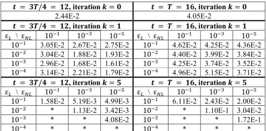
𝒕 = 𝟑𝑻/𝟒 = 𝟏𝟐, iteration 𝒌 = 𝟎 𝒕 = 𝑻 = 𝟏𝟔, iteration 𝒌 = 𝟎 2.44E-2 4.05E-2
𝒕 = 𝟑𝑻/𝟒 = 𝟏𝟐, iteration 𝒌 = 𝟏 𝒕 = 𝑻 = 𝟏𝟔, iteration 𝒌 = 𝟏 ε~ \ εT~ 10iX 10i¤ 10i¬ ε~ \ εT~ 10iX 10i¤ 10i¬
10iX 3.05E-2 2.67E-2 2.75E-2 10iX 4.62E-2 4.25E-2 4.36E-2
10i2 3.04E-2 1.88E-2 1.93E-2 10i2 4.40E-2 3.99E-2 3.84E-2
10i¤ 2.96E-2 1.68E-2 1.61E-2 10i¤ 4.25E-2 3.74E-2 3.52E-2
10i¼ 3.14E-2 2.21E-2 1.79E-2 10i¼ 4.96E-2 5.15E-2 3.71E-2
𝒕 = 𝟑𝑻/𝟒 = 𝟏𝟐, iteration 𝒌 = 𝟓 𝒕 = 𝑻 = 𝟏𝟔, iteration 𝒌 = 𝟓 ε~ \ εT~ 10iX 10i¤ 10i¬ ε~ \ εT~ 10iX 10i¤ 10i¬
10iX 1.58E-2 5.19E-3 4.99E-3 10iX 6.11E-2 2.43E-2 2.00E-2
10i2 * 1.13E-2 3.42E-3 10i2 * 1.10E-1 3.04E-2
10i¤ * * 4.08E-2 10i¤ * * 1.72E-1
10i¼ * * * 10i¼ * * *
Table 5: Second test case (flow around obstacles): relative error per iteration and instant for the ROM-based parareal
simulations using different thresholds ε~ (rows) and εT~ (columns) for the model reduction, for 𝑡 = 3𝑇/4 and 𝑡 = 𝑇,
and the zeroth, first and fifth parareal iterations. Errors in iteration 0 are the same for all the simulations and correspond to the error between 𝒢JH and ℱGH. Simulations with an asterisk were unstable and did not complete five iterations.
Iteration 𝒌 = 𝟏 Iteration 𝒌 = 𝟓
ε~ \ εT~ 10iX 10i¤ 10i¬ ε~ \ εT~ 10iX 10i¤ 10i¬
10iX 7.96 7.71 7.33 10iX 1.89 1.65 1.48
10i2 7.37 7.50 6.99 10i2 * 1.49 1.31
10i¤ 6.91 6.73 6.66 10i¤ * * 1.19
10i¼ 6.55 6.22 6.10 10i¼ * * *
Table 6: Second test case (flow around obstacles): speedup at the first and fifth iteration in function of the thresholds ε~
(rows) and εT~ (columns) for the ROM-based parareal simulations. Simulations with an asterisk were unstable and did
not complete five iterations.
4.2 Comparison between the variants of the parareal method
We consider the tests cases presented above for comparing the performance of the classical parareal method, the ROM-based one and our proposed modification. This comparison is made for fixed pairs of thresholds (ε~, εT~), and for different values of α for the enrichment of the snapshot sets.
4.2.1 1D flow with 𝜀~ = 𝜀T~ = 10i¬
As shown in Table 2, the ROM-based parareal method behaves well with ε~ = εT~ = 10i¬. Therefore, the
objective in using the snapshot enrichment is to have more precise results within less iterations. We perform simulations with α taking values in {1, 1/2, 1/4, 1/10, 1/200}, the first of these values corresponding to the non-enriched method and the last one to the smallest possible value for α, since 𝑝 = 200 (i.e. the snapshots are taken in every time step of the fine discretization).
Table 7 presents the error 𝑒Po for each parareal simulation, in the first and fifth iterations, and 𝑡 = 𝑇/2
and 𝑡 = 𝑇. We first notice that the classical parareal method is unstable in this simple test case, with an increasing error along iterations. Concerning the ROM-based simulations, we observe important improvements by enriching the model reduction, mainly for 𝑡 = 𝑇/2, where, in one iteration, the relative
method for speeding up the numerical resolution of the 2D shallow water equations error decreases from 10i¤ (in the non-enriched simulation) to 10i¬ approximately, with only one extra
snapshot per time step (α = 1/2). More but less remarkable improvements are observed for smaller α. The water depth at the final instant of simulation is presented in Figure 6 for some of the performed parareal simulations and compared to the referential solution. The unstable behavior of the classical parareal method is evident. For the ROM-based parareal method, without or with enrichment, the solutions at the first iteration are almost visually indistinguishable from the referential one. Finally, Figure 7 shows, for each simulation, the computational time and the speedup along iterations. The drawback of choosing a too large number of snapshots is evident for the cases α = 1/10 and α = 1/200, which are more expensive than the referential simulation after few iterations, with little accuracy improvement, as shown in Table 7. Therefore, α = 1 or α = 1/2 are reasonable choices for this test case, corresponding respectively to a speedup factor of approximately 4 and 3, respectively (in the first iteration, in which a high-quality solution is obtained).
Parareal method Iteration 𝒕 = 𝑻/𝟐 = 𝟐 𝒌 = 𝟏 Iteration 𝒌 = 𝟓 Iteration 𝒌 = 𝟏 Iteration 𝒌 = 𝟓 𝒕 = 𝑻 = 𝟒
Classical 3.37E-2 2.11E-2 3.75E-2 6.98E-2 ROM-based (α = 1) 8.76E-4 9.29E-7 1.01E-2 4.86E-6 ROM-based (α = 1/2) 1.70E-5 2.09E-9 6.31E-3 2.79E-6 ROM-based (α = 1/4) 1.01E-5 1.01E-8 6.58E-3 2.77E-6 ROM-based (α = 1/10) 4.38E-6 5.63E-10 7.21E-3 1.89E-6 ROM-based (α = 1/200) 4.48E-6 4.68E-10 7.37E-3 1.80E-6
Table 7: First test case (1D flow) with ε~= εT~= 10i¬: relative error per iteration and instant using the classical
parareal method and the ROM-based parareal method with different values of α, for 𝑡 = 𝑇/2 and 𝑡 = 𝑇, and the first and fifth parareal iterations.
Figure 6: First test case (1D flow) with ε~= εT~= 10i¬: water depth at the final instant of simulation (𝑇 = 4) along
the slice 𝑦 = 10 in iteration 0 (left figure), 1 (middle figure) and 2 (right figure) of the classical parareal method (squares), the ROM-based parareal with 𝛼 = 1 (crosses) and the ROM-based parareal with 𝛼 = 1/2 (ticks). The dashed line represents the referential solution. All the parareal solutions coincide in the 0-th iteration, since it corresponds to the coarse solution (given by 𝒢JH). The solutions are the same along any slice in the 𝑥 direction.
Figure 7: First test case (1D flow) with ε~= εT~= 10i¬: computational time (left figure) and speedup 𝑠(𝑘) (right
figure) for each parareal simulation. The dashed lines represent respectively the computational time for the simulation of the fine, referential solution, and a unitary speedup (no acceleration).
4.2.2 1D flow with 𝜀 = 10i¬ and 𝜀
T~ = 10i¤
Table 2 reveals that the ROM-based parareal method is unstable for ε~ = 10i¬ and ε
T~ = 10i¤; therefore,
method for speeding up the numerical resolution of the 2D shallow water equations The evolution of the errors presented in Table 8 shows smaller but still present instabilities for α ≤ 1/2, specially for advanced time steps. Also, taking smaller values of does not introduce significative quality gain. The water depth in the final instant of simulation, shown in Figure 8, evidences the unstable behaviour for α = 1. The computational times are similar to the previous test cases (with a small gain due to the reduction of εT~) and are omitted here. Therefore, in this test case α = 1/2 is the most effective choice, but it would be preferable to choose other values for ε~ and εT~.
Parareal method 𝒕 = 𝑻/𝟐 = 𝟐 𝒕 = 𝑻 = 𝟒
Iteration 𝒌 = 𝟏 Iteration 𝒌 = 𝟓 Iteration 𝒌 = 𝟏 Iteration 𝒌 = 𝟓 Classical 3.37E-2 2.11E-2 3.75E-2 6.98E-2 ROM-based (α = 1) 3.49E-3 2.06E-3 1.98E-2 1.61E-1 ROM-based (α = 1/2) 2.92E-3 1.51E-3 1.95E-2 1.05E-2 ROM-based (α = 1/4) 2.37E-3 8.99E-4 1.75E-2 9.73E-3 ROM-based (α = 1/10) 2.37E-3 3.85E-4 1.86E-2 7.96E-3 ROM-based (α = 1/200) 2.38E-3 6.68E-4 1.91E-2 1.36E-2
Table 8: First test case (1D flow) with ε~= 10i¬ and εT~= 10i¤: relative error per iteration and instant using the
classical parareal method and the ROM-based parareal method with different values of α, for 𝑡 = 𝑇/2 and 𝑡 = 𝑇, and the first and fifth parareal iterations.
Figure 8: First test case (1D flow) with ε~= 10i¬ and εT~= 10i¤: water depth at the final instant of simulation (𝑇 =
4) along the slice 𝑦 = 10 in iteration 0 (left figure), 1 (middle figure) and 2 (right figure) of the classical parareal method (squares), the ROM-based parareal with 𝛼 = 1 (crosses) and the ROM-based parareal with 𝛼 = 1/2 (ticks). The dashed line represents the referential solution. All the parareal solutions coincide in the 0-th iteration, since it corresponds to the coarse solution (given by 𝒢JH). The solutions are the same along any slice in the 𝑥 direction.
4.2.3 Flow around obstacles with 𝜀~ = 10i¤ and 𝜀T~ = 10i¬
We consider the thresholds ε~ = 10i¤ and ε
T~ = 10i¬ for simulating the second test case. Table 5 shows
an unstable behavior of the non-enriched ROM-based parareal method under these configurations. We consider the values in {1, 1/2, 1/4, 1/8, 1/16} for α.
Table 9 presents the relative errors 𝑒Po. The classical parareal method is unstable and produces negative
water depth from the third iteration. By enriching the snapshots sets, more stable solutions are obtained; a less important unstable behavior is still observed in the first iterations for the last time steps (mainly for the most enriched case, α = 1/16), but it is effectively controlled in the following iterations.
The physical behavior of the solution is illustrated in Figure 9 and Figure 10, showing the water depth along the slice 𝑦 = 47, respectively at 𝑡 = 3𝑇/4 = 12 and 𝑡 = 𝑇 = 16. In the former case, very good approximations to the referential solution are obtained after two iterations of the classical parareal methods and the enriched ROM-based ones, with 𝛼 = 1/2 and 𝛼 = 1/4. In the latter case, strong instabilities are produced in the classical and the non-enriched ROM-based methods, and three iterations of the ROM-based methods, specially for 𝛼 = 1/4, produce high-quality approximations. Finally, Figure 12 compares the referential solution (water depth, 𝑥-unit discharge and 𝑦-unit discharge in the entire domain) with the parareal one (ROM-based with α = 1/4), in the zeroth, first and third iterations.
Concerning the computational times, presented in Figure 11, speedup factors between 2 and 4, approximately, are obtained after two iterations for α = 1/2 and α = 1/4. For the third iteration, the
method for speeding up the numerical resolution of the 2D shallow water equations speedups are below 2. Therefore, more efficient implementations of the parareal method and the model reduction are necessary for improving the parallel efficiency of the algorithm.
Parareal method Iteration 𝒕 = 𝟑𝑻/𝟒 = 𝟏𝟐 𝒌 = 𝟏 Iteration 𝒌 = 𝟓 Iteration 𝒌 = 𝟏 Iteration 𝒌 = 𝟓 𝒕 = 𝑻 = 𝟏𝟔
Classical 2.72E-2 * 5.91E-2 * ROM-based (α = 1) 1.61E-2 4.08E-2 3.52E-2 1.72E-1 ROM-based (α = 1/2) 2.73E-2 8.58E-4 6.17E-2 1.16E-2 ROM-based (α = 1/4) 1.59E-2 8.27E-4 3.67E-2 9.19E-3 ROM-based (α = 1/8) 2.26E-2 1.46E-3 8.29E-2 3.44E-2 ROM-based (α = 1/16) 2.54E-2 6.31E-4 5.06E-2 1.30E-2
Table 9: Second test case (flow around obstacles) with ε~= 10i¤ and εT~= 10i¬: relative error per iteration and
instant using the classical parareal method and the ROM-based parareal method with different values of α, for 𝑡 = 3𝑇/4 and 𝑡 = 𝑇, and the first and fifth parareal iterations. The asterisk indicates that the classical method was unstable and did not complete five iterations.
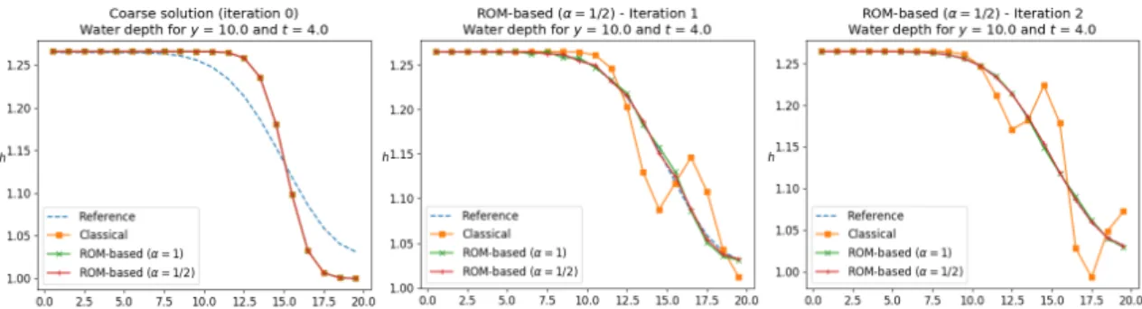
Figure 9: Second test case (flow around obstacles) with ε~= 10i¤ and εT~= 10i¬: water depth at 𝑡 = 3𝑇/4 = 12
along the slice 𝑦 = 47. Dashed curves represent the reference solution. Top: coarse solution (iteration 0); first column: classical parareal method; second column: ROM-based parareal with α = 1; third column: ROM-based parareal with α = 1/2; fourth column: ROM-based parareal with α = 1/4. Second row: iterations 1; third row: iteration 2; fourth row: iteration 3.
method for speeding up the numerical resolution of the 2D shallow water equations
Figure 10: Second test case (flow around obstacles) with ε~= 10i¤ and εT~= 10i¬: water depth at 𝑡 = 𝑇 = 16
along the slice 𝑦 = 47. Dashed curves represent the reference solution. Top: coarse solution (iteration 0); first column: classical parareal method; second column: ROM-based parareal with α = 1; third column: ROM-based parareal with α = 1/2; fourth column: ROM-based parareal with α = 1/4. Second row: iterations 1; third row: iteration 2; fourth row: iteration 3.
Figure 11: Second test case (flow around obstacles) with ε~= 10i¤ and εT~= 10i¬: computational time (left figure)
and speedup 𝑠(𝑘) (right figure) for each parareal simulation. The dashed lines represent respectively the computational time for the simulation of the fine, referential solution, and a unitary speedup (no acceleration).
4.CONCLUSIONS
In this paper, we implemented and compared some variants of the parareal method for speeding up the numerical resolution of the two-dimensional nonlinear shallow water equations. This method allows to pararellize in time a fine, expensive simulation in a predictor-correction iterative algorithm, in which the predictions are given by a coarser and less expensive model. The variant considered here uses reduced-order
method for speeding up the numerical resolution of the 2D shallow water equations models formulated on-the-fly with the POD and EIM techniques and allows to overcome the well-known stability and convergence issues for the method when applied to hyperbolic problems. We proposed a modification of the ROM-based parareal method consisting in the enrichment of the snapshots set used as input for the model reduction, with extra snapshots whose computation does not require any extra computational cost.
Figure 12: Second test case (flow around obstacles) with ε~= 10i¤ and εT~= 10i¬: water depth (left column), 𝑥-unit
discharge (middle column) and 𝑦-unit discharge (right column) at 𝑡 = 𝑇 = 16. First row: reference solution; second row: iteration 0 (coarse solution); third and fourth rows: iterations 1 and 3 of the ROM-based parareal method with α = 1/4.
A number of test cases with increasing complexity were performed for illustrating and studying the methods. Firstly, we studied the influence of the truncation thresholds for the formulation of the ROMs. The results show that the parareal method using ROMs with higher dimensions converges faster but may present unstable behaviors, due to the inaccuracy of the input snapshots. These instabilities can be partially
method for speeding up the numerical resolution of the 2D shallow water equations minimized by increasing the dimension of the reduced nonlinear term of the governing equations, however with a higher computational cost.
Secondly, we compared the classical parareal method, the ROM-based one and our proposed modification for different number of extra snapshots for the ROM enrichment. Our method provides, with few extra snapshots, more stable solutions and a faster decreasing of the relative error with respect to the reference solution. Further increments on the number of snapshots provide more but less remarkable improvements, with the drawback of a prohibitive computational time: even if the computation of the extra snapshots is costless, the model reduction has a quadratic cost relative to the number of input snapshots.
Therefore, the enriched ROM-based parareal method, with few extra snapshots, is able to provide good and stable approximations of the fine, referential solution with a smaller computational time. Speedup factors up to 3 were obtained in the simulations presented along this paper. Thus, the method shows itself as a promising alternative for speeding up the resolution of the SWE and other problems in hydrodynamics. Moreover, further improvements in the speedup could be obtained with more efficient implementation of the parareal method and the model reduction procedures.
REFERENCES
[1] J.-L. Lions, Y. Maday and G. Turinici, “Résolution d’edp par un schéma en temps 'pararéel',” Comptes
Rendus de l’Académie des Sciences - Series I - Mathematics, vol. 332, no. 7, pp. 661-668, 2001.
[2] D. Ruprecht, «Wave propagation characteristics of Parareal,» Computing and Visualization in Science, vol. 9, pp. 1-17, 2018.
[3] A. J. C. Barré de Saint-Venant, «Théorie du mouvement non permanent des eaux, avec application aux crues des rivières et à l'introduction des marées dans leur lit,» Comptes Rendus des Séances de
l'Académie des Sciences, vol. 73, pp. 147-154 and 237-240, 1871.
[4] F. Chen, J. S. Hesthaven y X. Zhu, «On the Use of Reduced Basis Methods to Accelerate and Stabilize the Parareal Method,» de Reduced Order Methods for Modeling and Computational Reduction, Cham, 2014.
[5] G. Bal y Y. Maday, «A 'parareal' time discretization for non-linear ODE's with application to the pricing of an American put,» de Recent Developments in Domain Decomposition Methods, 2002.
[6] M. Astorino, F. Chouly y A. Quarteroni, «Multiscale coupling of finite element and lattice Boltzmann methods for time dependent problems.,» 2012.
[7] M. Barrault, Y. Maday, N. C. Nguyen y A. T. Patera, «An 'empirical interpolation' method: application to efficient reduced-basis discretization of partial differential equations,» Compres Rendus
Mathématiques, vol. 339, nº 9, pp. 667-672, 2004.
[8] S. Chaturantabut y D. C. Sorensen, «Nonlinear model reduction via discrete empirical interpolation.,»
SIAM Journal on Scientific Computing, vol. 32, nº 5, p. 2737–2764, 2010.
[9] R. Narasimha, «Kosambi and proper orthogonal decomposition,» Resonance, vol. 16, pp. 574-581, 2011.
[10] R. Camphouse, J. Myatt, R. Schmit, M. Glauser, J. Ausseur, M. Andino y R. Wallace, «A snapshot decomposition method for reduced order modeling and boundary feedback control,» de 4th AIAA Flow
Control Conference, 2008.
[11] C. W. Rowley, T. Colonius y R. M. Murray, «Model reduction for compressible flows using POD and Galerking projections,» Physica D: Nonlinear Phenomena, vol. 189, nº 1, pp. 115-129, 2004.
[12] C. W. Rowley, «Model reduction for fluids, using balanced proper orthogonal decomposition,»
International Journal of Bifurcation and Chaos, vol. 15, nº 3, pp. 997-1013, 2005.
[13] J. Borggard, Z. Wang y L. Zietsman, «A goal-oriented reduced-order modeling approach for nonlinear systems,» Computers & Mathematics with Applications, vol. 71, nº 11, pp. 3155-2169, 2016.
[14] J. G. Caldas Steinstraesser, V. Guinot y A. Rousseau, Modified parareal method for solving the two-dimensional nonlinear shallow water equations using finite volumes.