Detecting Corrosion in Aircraft Components
Using Neutron Radiography
by
David Walter Fink
Submitted to the Department of Nuclear Engineering
in partial fulfillment of the requirements for the degree of
Master of Science
at the
MASSACHUSETTS INSTITUTE OF TECHNOLOGY
January 1996
@ Massachusetts Institute of Technology 1996. All rights reserved.
OF TECHNOLOGY
APR 2 2 1996 5ý
Author
LIB... RARESDepartment of Nuclear Engineering
January 18, 1996
Certified by
...
Richard Lanza
Principal Research Scientist
Thesis Supervisor
Read by
...
Lawrence Lidsky
Professor of Nuclear Engineering
Thesis Reader
A ccepted by ...
-/
V
/Jeffrey Freidberg
Detecting Corrosion in Aircraft Components Using
Neutron Radiography
by
David Walter Fink
Submitted to the Department of Nuclear Engineering on January 18, 1996, in partial fulfillment of the
requirements for the degree of Master of Science
Abstract
This work involved testing an accelerator based neutron radiography imaging system. The neutron source was a DL-1 radiofrequency quadrupole accelerator from AccSys technologies used to accelerate deuterium ions to 975 keV, producing neutrons in the
9Be(d, n)B'0 reaction. The goal of this work was to demonstrate the capability of
the relatively new RFQ accelerator to provide a compact, mobile neutron source with an intensity sufficient for imaging purposes. Neutron production rates of up to 8.8E8 - were achieved with the DL-1 source, with a thermal neutron flux of 1.3E4 n at
S C 28
2
the imaging plane. A mobile neutron source of this strength widens the applications possible for neutron radiography.
The imaging system used was a thermal neutron scintillator that was lens coupled to a cooled, charge coupled device. This provides a very low noise imaging system. The maximum signal level of the imaging system is 3.27E4 counts per pixel, with a readout noise of 76.7 counts per pixel and a dark current noise of less than 1 count per pixel per second.
Noise sources affecting the imaging system were investigated and minimized. The system capabilities were tested by imaging phantoms of known internal structure. The ability to use this system to image corrosion in aircraft components was tested by using the system on pieces of aircraft skin from actual aircraft with successful results.
Thesis Supervisor: Richard Lanza Title: Principal Research Scientist
Acknowledgments
There are many people without whom this work could not have been completed. First I would like to thank Dr. Richard Lanza for his help and guidance. His boundless energy and enthusiasm kept my work exciting and fun. He showed amazing patience when nothing seemed to work, true insight in solving many technical problems which barred my way, and genuine excitement at even the tiniest bit of progress. He showed me the true joy that can be gained in the process of discovering.
I thank my thesis reader, Dr. Lawrence Lidsky, for his suggestions and help with this work, as well as his patience and understanding.
I would like to thank Erik Iverson and Shuanghe Shi for their help. I cannot recall how many times Erik's helpful suggestions saved me vast amounts of time and inconvenience. His valuable help as electrical engineer, plumber, computer scientist, and accelerator repairman, and brewmeister cannot be measured.
I thank the many faculty members who selflessly offered guidance and equipment. I would especially like to thank Dr. Kevin Wenzel for answering innumerable ques-tions that began with "Do you know where I can find a . ."
I thank the Lab for Nuclear Science Machine Shop for helping me in countless numbers of situations. Without their excellent craftsmanship many of the repairs re-quired to keep our equipment operating would not have been possible and this work simply could not have been completed.
I would like to thank the Air Force Office of Scientific Research for providing the financial support for this project, and the U. S. Navy for giving me the time to com-plete this work. I offer my very respectful thanks to Rear Admiral Ray Smith for supporting my desire to continue my education.
Finally, I would like to thank the people who, although they did not contribute directly to this work, were special to me in other ways. I would like to thank my roommate, Jon Lunglhofer, for being a true friend and dragging me up climb after climb. You introduced me to the vertical world, which will always be part of my life. For that, and putting up with me for almost two years, I thank you. Keep cranking hard.
I thank my girlfriend Carol Berrigan for supporting me and being there for me no matter how irritable or impatient I got. I love you.
I thank my parents, Harvey and Barbara Fink, for their unconditional love and support. Without them I wouldn't be where I am today. I love you.
Contents
1 Introduction
1.1 G oals . . . . 1.2 Contributions of This Thesis . . . . 1.3 Organization of This Work . . . . 2 General Properties of Radiography
2.1 History of Radiography ... 2.2 Theory of Radiography ...
2.2.1 Requirements for Radiography . . . . 2.2.2 Fluence Requirements for Radiography . . . . 2.3 Spatial Resolution of Imaging Systems . . . . 2.4 Neutrons vs. X-Rays ...
2.4.1 Applications Suited to Neutron Radiography . . . .
3 Radiography of Corrosion in Aircraft Structures
3.1 Costs Associated with Corrosion ...
3.2 Corrosion of Aluminum Aircraft Structures . . . . 3.2.1 Corrosion Products ...
3.2.2 Types of Corrosion ...
3.3 Non-Destructive Evaluation of Corrosion in Aircraft Structures . 3.3.1 Benefits of NDE to the Airline Industry . . . .
3.3.2 Aging Aircraft Concerns ...
3.3.3 Present State of Non-Destructive Inspection of Aircraft .
13 13 14 14 30 .. . 30 . . . 31 .. . 32 .. . 32 . . . 35 . . . 35 .. . 35 . . . 36
3.3.4 Neutron Radiography and Detection of Corrosion in Aircraft Structures
4 Detector Configuration and Characteristics 4.1 Theory of Position Sensitive Neutron Detection
4.1.1 Gas Detectors ... 4.1.2 Scintillator Methods . . . . 4.1.3 Film Methods ... 4.2 Detector Configuration . . . . 4.3 Scintillator ... 4.4 Cam era ... 4.4.1 Efficiency of CCD ... 4.4.2 CCD Noise Characteristics . . . . . 4.4.3 Camera Gain ... 4.5 Detector Response . . . . 4.5.1 Dynamic Range . . . . 4.6 Spatial Resolution of Imaging System . . .
5 Neutron Source
5.1 Overview of Types of Neutron Sources 5.1.1 Reactor Sources ...
5.1.2 Accelerator Sources ... 5.1.3 Isotope Sources ...
5.2 Radiofrequency Quadrupole Accelerators . 5.2.1 Theory ...
5.2.2 Focusing ...
5.3 DL-1 Neutron Source Characteristics . . . 5.3.1 Accelerator Components . . . . 5.3.2 Neutron Production ... 5.4 Flux Measurements ... . . . . 78 . . . 37 40 . . . . . 40 . . . . 41 . . . . . 42 . . . . 42 . . . . . 43 . . . . 43 . . . . 45 . . . . 46 . . . . . 46 . . . . 53 . . . . . 55 . . . . . 59 . . . . . 59 61 . . . . . 61 . . . . 61 . . . . 62 . . . . 65 . . . . . 66 . . . . 66 . . . . 66 . . . . . 70 . . . . . 71 . . . . 73 . . . . 78 5.4.1 Camera Method..
5.4.2 GS-20 Measurements ... 79
5.4.3 Results ... .... ... ... ... .. 80
6 Radiographs of Known Phantoms 83 6.1 Radiography Procedure ... 83
6.1.1 Measuring the Neutron Flux ... 84
6.1.2 Sample Exposure ... 84
6.1.3 Blank Screen Exposure ... 85
6.1.4 Dark Current Exposure ... .. 86
6.1.5 Correcting for Non-uniform Flux . . . . 86
6.2 Types of Phantoms ... ... 87
6.2.1 Corroded Aluminum Samples . ... 88
6.2.2 Polyethylene Phantom . . . . 92
6.3 Aluminum Hydroxide Phantom . . . . ... . . . . 97
6.4 Wax Phantom ... .. ... ... ... .. 100
7 Radiographs of Aircraft Components 104 7.1 Lap Joint 1 .... ... . 106 7.2 Lap Joint 2 ... ... . 108 7.3 Lap Joint 3 ... . 111 8 Conclusions 113 8.1 System Weaknesses ... 113 8.1.1 Noise Sources .. .... ... ... 113 8.1.2 Collim ation ... 114 8.1.3 Corrosion vs. Epoxy ... . 114 8.2 System Strengths ... ... ... .. 115 8.2.1 Portable System ... .... .... .... .. 115 8.2.2 Source Strengths ... ... . 116 8.2.3 Detector Strengths ... ... .... .. 116 8.2.4 Time Considerations ... ... . 117
8.3 Future Development ... ... ... . ... . .. . .. .. 117
8.3.1 Moderator Design ... . . . . 117
8.3.2 Collimation ... . . . . . . 118
8.3.3 Quantify the Noise Response . ... . . . 118
List of Figures
2-1 Importance of Collimation for Spatial Resolution . . . . 2-2 Importance of Detector Spatial Resolution for Radiography . . . . 2-3 Object Containing Two Materials with Similar Radiation Attenuation 2-4 2-5 2-6 3-1 3-2 3-3 Properties . . . . Edge Function ...
Derivative of Edge Function ...
Neutron vs Photon Attenuation Characteristics Photograph of Aloha Airlines Flight 243 . . . . Pourbaix Diagram for Aluminum . . . . Chemistry of a Corrosive Pit . . . .
. . . . 20 . . . . 25 . . . . 26 . . . . . 27 . . . . 44 . . . . . 46 4-1 Components of Imaging System ...
4-2 CCD Efficiency vs Photon Energy . . . . 4-3 4-4 4-5 4-6 4-7 5-1 5-2 5-3 5-4
Mean Pixel Level, Shielded and Unshielded CCD, 9.1 uA Beam Current Mean Pixel Level, Shielded and Unshielded CCD, 40.0 uA Beam Current Dark Current Exposure vs. Time ...
Camera Gain Curve ... MTF of Imaging System ...
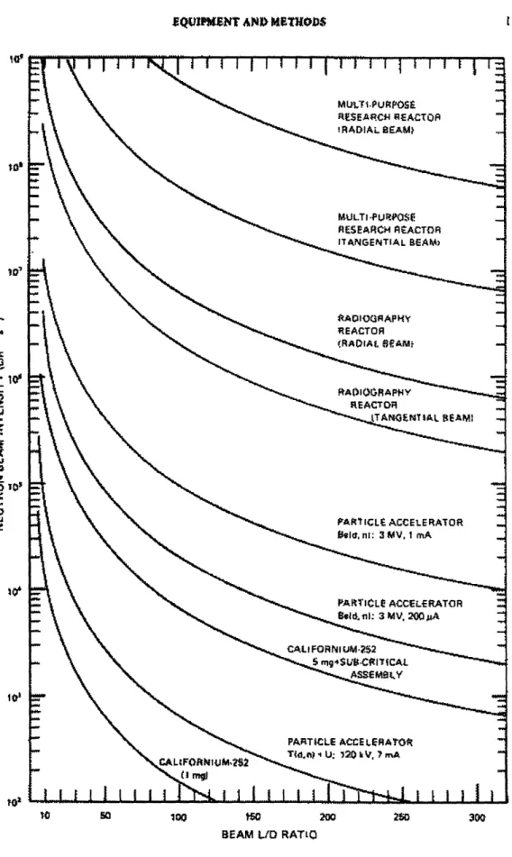
Comparison of Neutron Source Strengths . . . . Neutron Yeild for Various Reactions vs Incident Energy . . . . Time and Space Variation of Electric Quadrupole . . . . Alternating Focusing and De-Focusing Fields . . . .
5-5 Electric Field Normal to Beam Direction . ... 68
5-6 Electric Field Along Beam Direction . . . . 69
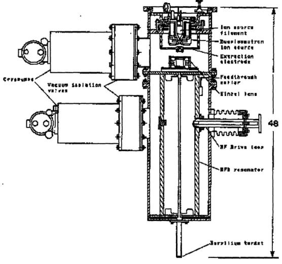
5-7 Ion Source and Accelerator Cavity . . . . 72
5-8 Neutron Production Spectrum from 1MeV Deuterons on Beryllium . 74 5-9 Target Position and Shielding ... .76
5-10 Absolute Efficiency of GS-20 vs Neutron Energy . . . . 80
6-1 2 Minute Blank Screen Exposure, Pixels Grouped 4x4 . . . . 86
6-2 Photograph of Corrosion Sample Phantom . . . . 88
6-3 Radiograph of Corrosion Sample Phantom, 2 Minute Exposure, 4x4 Pixel Grouping ... 89
6-4 Median Filtered Image of Corrosion Sample Phantom . . . . 90
6-5 Graph of Average ADC Value of Filtered Image vs Vertical Position . 91 6-6 Photograph of Polyethylene Phantom . . . ... . . . . 93
6-7 Unfiltered Radiograph of Polyethylene Phantom, 2 Minute Exposure, 4x4 Pixel Grouping ... 94
6-8 Median Filtered Radiograph of Polyethylene Phantom, 2 Minute Ex-posure, 4x4 Pixel Grouping ... .. 95
6-9 Photograph of Aluminum Hydroxide Phantom ... . . . . 97
6-10 Aluminum Hydroxide Phantom, Median Filtered Radiograph, 2 Minute Exposure 4x4 Pixel Grouping . . . . .. . . . .. . . . 98
6-11 Average ADC Value of Each Column of Figure 6.10 vs Horizontal Position 99 6-12 Photograph of Wax Phantom ... 101
6-13 Median Filtered Image of Radiograph of Wax Phantom, 100s exposure, 4x4 Pixel Grouping ... .. . 101
6-14 Average ADC Value of Each Column in Figure 6.13 vs Position . . . 102
7-1 Diagram of a Typical Lap Joint . . . . ... . .. . . . . 105
7-2 Photograph of Lap Joint 1 (Front View) . . . 106
7-3 Photograph of Lap Joint 1 (Side View) . . . 107
7-5 Radiograph of Lap Joint 1 ... . . . . . . . . 109
7-6 Photograph of Lap Joint 2 (Front View) . . ... .... . 109
7-7 Photograph of Lap Joint 2 (Side View) ... . . . . . 110
7-8 Radiograph of Lap Joint 2 . . . . ... . . . . ..... . 110
7-9 Photograph of Lap Joint 3 (Front View) . . . ... . . . . . 111
List of Tables
3.1 Aging Aircraft Summary ... ... 36
3.2 Cross Sections of Various Elements for X-Rays and Neutrons in barns (10- 24cm2) ... ... 38
3.3 Linear Attenuation Coefficients for Aluminum and Corrosion Products for X-Rays and Neutrons (cm-' ) . ... . . . . 39
3.4 • for Corrosion Products in Aluminum for Different Radiation Types 39 4.1 Average Pixel Exposure, Shielded and Unshielded CCD ... 48
4.2 Dark Current Data ... 51
4.3 Gain Curve Data Points ... 55
5.1 Isotope Neutron Source Characteristics . ... 65
5.2 DL-1 Source Characteristics ... 71
5.3 DL-1 Source Strength Data ... 81
5.4 Neutron Flux at Scintillator Screen . ... 82
6.1 Mean Pixel ADC Value of Regions of the Polyethylene Phantom . . . 96
6.2 Neutron Attenuation of Regions of Polyethylene Phantom ... 96
6.3 Mean Pixel Level of Regions of the Wax Phantom . ... 103
6.4 Predicted and Measured Neutron Attenuation of Regions of Wax Phan-tom . . . .. . . . .. 103
Chapter 1
Introduction
1.1
Goals
Neutron radiography is a technique that has been proven to be an effective method for the non-destuctive evaluation of materials in a number of fields. It's applications, however, have been severely limited by the fact that neutron sources of sufficient strength were limited to fixed, expensive, and exceedingly complex nuclear reactors. Recent developments in ion accelerator technology have made cheaper, more compact accelerators with higher currents available for use in neutron generators.
These new, smaller, higher current accelerators have made portable neutron sources with sufficient intensity for radiography a reality. The reality of a mobile neutron source capable of generating the neutron flux required for imaging has opened many new applications to neutron radiography.
One of these applications is imaging corrosion in aluminum aircraft components. The main thrust of this work was to demonstrate the capability of one of these mo-bile neutron sources for imaging corrosion in aluminum. A commercially available, accelerator based neutron source was used along with an imaging system composed of commercially available components. The performance of this combined system was tested on phantoms whose composition was known and pieces of aircraft skin.
1.2
Contributions of This Thesis
The first contribution of this thesis was the characterization and mitigation of sources of noise in the imaging system used. It was found that photons produced from the neutron source caused noise in the imaging system, and that shielding components of the system with lead mitigated this noise.
A second contribution of the thesis was the use of phantoms of known content to characterize the performance of the imaging system. Specifically, signal attenuation and spatial resolution were investigated using phantoms of known hydrogen content in an aluminum matrix.
Finally, the ability of the system to image epoxy and corrosion in components taken from aircraft was demonstrated. A number of pieces of aircraft skin were ob-tained and radiographed. The results show the ability of this system to locate hidden corrosion and epoxy in aircraft components.
1.3
Organization of This Work
Chapter Two provides an introduction to tradiography theory and technique. It provides some of the physics that govern radiography and mathematics that govern imaging systems. Some brief historical notes and past uses of radiography are out-lined.
Chapter Three describes why corrosion of aircraft components is a topic of growing concern and importance. A number of reasons for having a quick and reliable method for detecting corrosion of aluminum aircraft components are discussed. Additionally,
the chemistry of aluminum corrosion is detailed, indicating why neutron radiography is a valid technique for detecting this corrosion.
Chapter Four is a description of the imaging system used in this work. A brief overview of types of position sensitive neutron detectors is given. Each of the com-ponents of the imaging system is discussed. Characteristics of the entire imaging system such as spatial resolution, noise, dynamic range, and detector efficiency are characterized.
Chapter Five is a discussion of the neutron source. The advantages and disad-vantages of the three basic types of neutron source (reactor, accelerator, isotope) is given. A brief outline of the theory behind radiofrequency quadrupole accelerators is included. Specific characterization of the DL-1 source characteristics, such as source strength and neutron spectrum produced, is provided.
Chapter Six details how the phantoms used to test the system were created. It also contains the reults of using the imaging system on these phantoms. The actual results are compared to the results predicted by theory.
Chapter Seven describes the samples of aircraft skin used to test the system and the radiographs of those samples.
Chapter Eight contains the conclusion reached doing this work and suggestions for future work related to this imaging system.
Chapter 2
General Properties of
Radiography
2.1
History of Radiography
Radiography is an imaging technique that has been as a non-destructive method for the evaluation of materials. The earliest use of radiography occurred the first time someone held an object up to a bright light to determine what was inside it. This is obviously an exceedingly simple case, but it is radiography, i.e. a projected shadow image.
The first use of a more technical form of radiography came with the discovery of x-rays by Roentgen in 1895[17, p. 1]. He found that a electron beam device caused exposure of photographic film. Roentgen also found that placing different materials between the electron tube and the film would sometimes form a shadow image of the object on the film. We now know that the film exposure was caused by x-rays, and the reason different materials altered the amount of exposure seen in the film was that these different materials stopped some of the x-rays, preventing them from reaching the film. This was later put to use in medicine when it was discovered that flesh was more easily penetrated by x-rays than bone, causing the two to show up with different intensities on photographic film.
The neutron was not discovered until 1932 by Chadwick[17, p. 1]. Problems with neutron sources and neutron detectors prevented investigation of neutron radiography until 1948, when Kallman began to research the possibilities[22]. Industrial applica-tions of the technique were explored by Thewlis in 1956[35] and continued by Berger in 1985[4].
Until recently, these industrial applications were limited by the fact that the only neutron sources strong enough to allow neutron radiography were nuclear reactors. This meant that samples to be radiographed had to be small enough to be trans-ported into an existing reactor, and shipping costs would add to the cost of testing. Additionally, the early techniques for imaging neutron beams were rather complicated and involved a number of steps. They took a long time and did not have very good resolution.
Neutron radiography has been used in the past to image:
* Distribution of explosives in pyrotechnics (ammunition and shells) * Gaps in seals and sealants
* Bond voids
* Corrosion, moisture, and hydrogen content in metals * Nuclear fuel rods
* Welds
* Hydrocarbon fuels and lubricants[16, p. 71] * Electronics[25, p. 81]
These uses of neutron radiography prove that it is a useful and viable technology. However, more widespread application of this technology has been limited by the fact
incident object detector incident object detector radiation
radiation response response
(a) (b)
Figure 2-1: Importance of Collimation for Spatial Resolution
that it requires an fixed neutron source (a nuclear reactor) and the need for improved neutron imaging systems.
2.2
Theory of Radiography
Radiography is the process of creating a projected shadow image. Radiation is passed through an object, and the spatial distribution of the radiation flux on the opposite side of the object was the "projected shadow." Differences in the amount of radiation that pass through the object at different positions indicate different material proper-ties of the object at different positions.
2.2.1
Requirements for Radiography
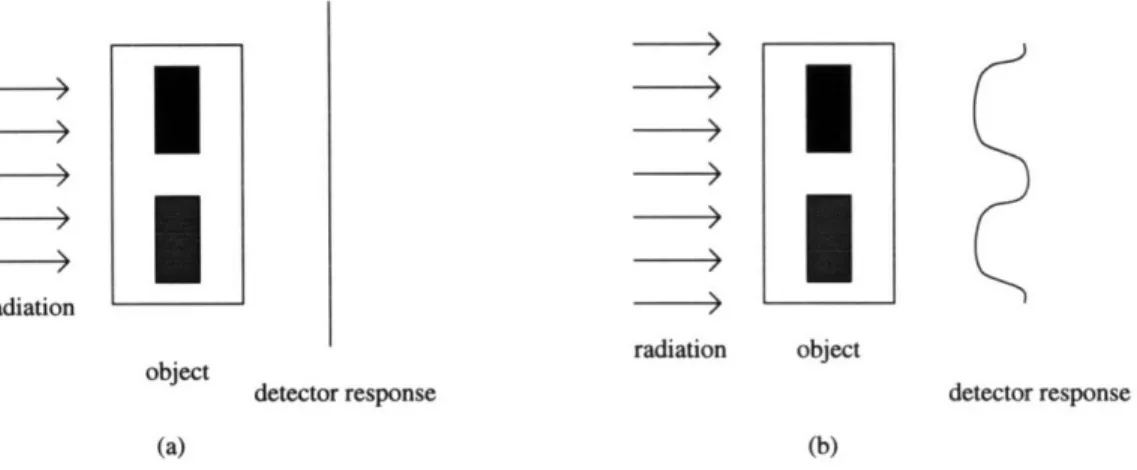
Collimation
One requirement for good radiographic imaging is that the radiation is well collimated. If the radiation is not collimated, image resolution is lost. The difference between the image formed using a highly collimated beam and using a beam with poor collimation is displayed in Figure 2.1.
I
detail detail
I
incident object detector incident object detector
radiation
radiation (a) response (b) response
Figure 2-2: Importance of Detector Spatial Resolution for Radiography using this source shows the clean, sharp edges of the interior detail. The uncollimated beam (Figure 2.1b) blurs the edges of the detail in the image due to radiation passing through the object at different angles. This problem is accentuated for thicker objects and systems with larger distances between the object and the detector.
Detector
Radiography also requires a position sensitive detector with a high spatial resolution. If the detector does not have high spatial resolution, the image will be blurred. In Figure 2.2a one can see how a detector with a high resolution can show the sharp edge of the detail and represent its size accurately. Figure 2.2b shows a detector with large pixel size. The detail in the object smaller than the detector pixel cannot accurately
be imaged. It appears as a larger, less dense detail than it actually is due to the detector pixel size.
Radiation
Radiography also requires certain characteristics of the radiation attenuation through the object. First, the radiation must be able to penetrate the bulk object. Otherwise, the detector response is zero for all positions, as illustrated in Figure 2.3a. Second, there must be a difference of attenuation through materials that one wishes to
dis-19
I
raiauIon
I
I
-7-I:
I UIUII U~ [IUIarLUll UUJcULobject detector response detector response
(a) (b)
Figure 2-3: Object Containing Two Materials with Similar Radiation Attenuation Properties
tinguish between. If the radiation is attenuated the same amount by two different materials, it is impossible to distinguish between them by looking at the detector re-sponse. Both appear as equally dark spots on the image. Figures 2.3a and 2.3b each show an object with two different materials inside of it. Each material has the same attenuation properties as the other, so they appear the same on the image. Figure 2.3b shows the identical detector response to two different materials with the same attenuation characteristics.
2.2.2
Fluence Requirements for Radiography
The fluence required to form a radiographic image depends on many factors, includ-ing the size of the details one wishes to image, the efficiency of the detector, the attenuation of the bulk object, the difference in attenuation between the detail and the bulk object, and the desired signal to noise ratio.
The mathematical relationship between these factors is relatively easy to derive. First, realize that the signal generated is simply the difference in the detected flux between the detail and the rest of the object.
signal = 4(e -pD - e-1(D - A ) e - (A+JA)(Ar] x) ) (2.1)
Where:
* ( = total fluence (particles/unit area)
* D = thickness of object
* p = attenuation coefficient of bulk object * Ax = size of detail to be imaged
* fp + /iC = attenuation coefficient of detail to be imaged
* 7 = detector efficiency
If we assume a well collimated beam and a perfect detector, the only noise present is due to statistical variation of the number of detected neutrons. Assuming that the beam conforms to Poisson statistics, the noise is easily characterized.
noise = 1ire-ID (2.2)
Define the signal to noise ratio, T, and simplify:
/ ( t)2AX4,q
O
='
(2.3)
epD
Rewriting this equation to express the required fluence to image details of a given size with a specific signal to noise ratio yields:
Jl!2eIpD
= () 2A (2.4)
(6p)2A,4X7
Equation 2.4 shows that fluence must be increased dramatically to image smaller and smaller objects (as Ax decreases, P increases rapidly). Additionally, as attenuation through the bulk object increases (pD increases), the required fluence increases. As
the difference in attenuation between the detail and the bulk object increases (6A increases), the required fluence drops rapidly.
2.3
Spatial Resolution of Imaging Systems
An imaging system may be thought of mathematically as an operator that acts on a function representing the physical object and returns a function that we call the image.
g(x, y) = S[f(X, y)]
(2.5)
Where:
* g(x,y) = image function * f(x,y) = object function
* S[f] = imaging system
As an example consider a medical x-ray. The physical object is some part of a human body, perhaps an arm. The function f(x,y) would be the distribution of x-ray attenuation coefficients in the arm. The image function g(x,y) would consist of the brightness of the photographic film at position (x,y).
Definition of a Linear, Stationary System
One type of imaging system is a linear, stationary system. These systems are math-ematically easier to analyze and are used for many imaging applications. Linear, stationary systems are more tractable mathematically because the image function, g(x,y), is the superposition of the imaging system function acting on each point of the object function (definition of linear system), and the imaging system function is identical for each point in the object function (definition of stationary system).
Using these two properties, we can rewrite equation 2.5:
g(x, y) =
f
f(x, y)h(x - xi, y - yi)dxldy (2.6)g(x, )
=
f(x -Xz, y -y)h(x, y)dxidyi
(2.7)
Where:
* (x,y) = position in image space * (xl, yl) = position in object space. * g(x,y) = image function
* f(xl, yl) = object function
* h(x,y;xl, yi) = mapping function
Here we have replaced the imaging system function, S[f(x,y)], with the linear superposition (sum) of the imaging system acting on each point in the object function. Because the system is stationary, the imaging system function is identical for each point in the object function. We have replaced the imaging system function S[f(x,y)] with h(x,y), where:
h(x, y) = S[56(z, yi)] = S[6(X2, y2)] = S[6(x3, Y3)]... (2.8)
Thus, h(x,y) is simply the result of the imaging system acting on a point. For this reason, h(x,y) is called the point spread function, or PSF. Equation 2.7 shows that the image function, g(x,y), is simply the convolution of the PSF, h(x,y) and the
object function, f(x,y).
Frequency Domain and Edge Response
We may change the convolution encountered in equation 2.7 into a simple multiplica-tion by taking the Fourier Transform of equamultiplica-tion 2.7. The two dimensional transform of any function f(x,y) is defined as:
F(kX, k,) =
f(x,
y)e-i(kx+kyy)dxdy (2.9)where:
* F(kx, ky) = Fourier Transform of f(x,y)
* (ks, ky) = Frequency domain coordinates corresponding to (x,y) in the position domain
Taking the Fourier Transform of equation 2.7 yields:
G(kx, ky) = F(kx, ky)H(kx, ky) (2.10) The convolution has been replaced with multiplication. Thus, a useful function to characterize a system is the Fourier transform of the point spread function. However, because it is difficult to create a true "point" object to measure the point spread function, systems are usually defined by a line response function.
The line response function (LRF) is defined as the point spread function (PSF) integrated over one variable:
1(X) =
J
6(x1 - xo)h(x, y)dsidy, (2.11)1(x) = h(xo, yi)dyi (2.12)
where:
* 1(x) = line response function * 6(x) = line at x = xo
* h(x,y) = point response function
The line response function is much easier to measure experimentally. All that is required is an edge of material that is opaque to the imaging radiation used for the system. This "edge" can be represented mathematically as an object function:
f(x,y) = 1
Xo
Figure 2-4: Edge Function
f(X, y) = Of orz < xo
(2.1
f (x, y) = f orx > x0o (2.1
By taking the derivative of the edge response, we can obtain the line response.
d Sf(x, y) = Oforx > xo, x < xo (2.1 dx d xf (, y) = If orx = Xo (2.1 d
+f(x, y) = f'(x, y) = 6(x -xo)
(2.1
Let the edge response be represented mathematically as e(x):
e(x)
=
f
(x,y)h(xi, yl)dxldyi
(2.1
Taking the derivative of the edge response with respect to x yields:
3)
4)5)
6)
7)
8)
f'(x,y) = 0
Xo
Figure 2-5: Derivative of Edge Function
de(x) = //f(, y)h(xl, yl)dxldyi (2.19)
-e(x) = Jf'(x, y)h(xi, yl)dxidyi (2.20)
e'(x) = 6(x - o)h(x1, yl)dxrdyi (2.21)
e'(x) = 1( )
(2.22)
2.4
Neutrons vs. X-Rays
In order to determine which type of radiation is best suited for a particular imaging application, one must keep in mind the requirements for radiography previously dis-cussed in section 2.2.1. We determined that in the ideal case the radiation used would penetrate the bulk object unattenuated, and that 6[ would be as high as possible. These two characteristics would minimize the fluence required to image objects with a specified resolution with a specified signal to noise ratio (see equation 2.4).
f'(Xo) = 1
7
ATOMIC NUMBER
Figure 2-6: Neutron vs Photon Attenuation Characteristics
Interactions of X-Rays with Matter
Photons interact with matter mostly through interactions with atomic electrons. This means that photon attenuation is highly dependent on electron density, which in-creases with atomic number Z and material density. Thus a x-ray radiograph yields information primarily regarding the electron density of the object.
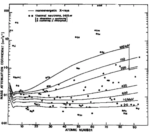
Photon attenuation also depends on photon energy. Figure 2.6 shows a plot of the attenuation coefficient vs. atomic number for photons ranging in energy from 100 keV to 2 MeV. The general trend of increasing attenuation with increasing atomic number can easily be seen, especially in the lower energy photons. Another important feature is that attenuation decreases with increasing photon energy and becomes less dependent on atomic number.
Interactions of Neutrons with Matter
Neutrons interact with matter in a much different way than x-rays. Neutrons almost never interact with atomic electrons; instead they are much more likely to interact with the nucleus. The result is that neutron attenuation varies a great deal from nucleus to nucleus. Looking at Figure 2.6 one can see that neutron attenuation coef-ficients vary over a much wider range of the logarithmic vertical axis than the x-ray attenuation coefficients. This nuclear interaction means that a neutron radiograph yields information regarding the isotopic content of the object imaged; an x-ray ra-diograph only gives information about electron density.
2.4.1
Applications Suited to Neutron Radiography
Inspecting Figure 2.6, one can easily see why neutron radiography was used for the applications listed at the beginning of this chapter. All involve the imaging of a hy-drogen containing material in a metal matrix. Hyhy-drogen is present in the explosives inside of a metallic shell casing, in the rubber or organic seal used in most seals and sealants, in the epoxy used to form bonds between metals or other materials, in many corrosion products found trapped in metallic matrices, in water which may leak into cracks in the metal cladding of nuclear fuel rods, and in the fuels and lubricants used in metallic engines.
Figure 2.6 indicates that hydrogen has a very large neutron cross section, and most structural metals (Al, Fe) have much lower neutron cross sections. This relationship is reversed for low energy x-rays, which show a low cross section for hydrogen and a high cross section for most metals. The x-rays are heavily attenuated in the metals, making them a poor choice for imaging details within metal structures. The x-ray cross section for metals drops with increased x-ray energy allowing penetration of metallic objects, but higher energy x-rays present a different problem. They show a relatively uniform attenuation coefficient for all materials, meaning Sl/ is small.
Neu-trons are clearly a much better choice for imaging hydrogen containing compounds in metals than x-rays.
Chapter 3
Radiography of Corrosion in
Aircraft Structures
3.1
Costs
Associated with Corrosion
Corrosion is defined as "destructive attack of a metal by chemical or electrochemical reaction with its environment." [36, p. 1] Corrosion costs impact industry in many ways; one cost is from repair and replacement of parts that must be replaced due to corrosion. Another cost is time and product lost due to a work stoppage caused by equipment failure due to corrosion or maintenance required due to corrosion. Corro-sion also costs money in the form of inspection and preventative maintenance.
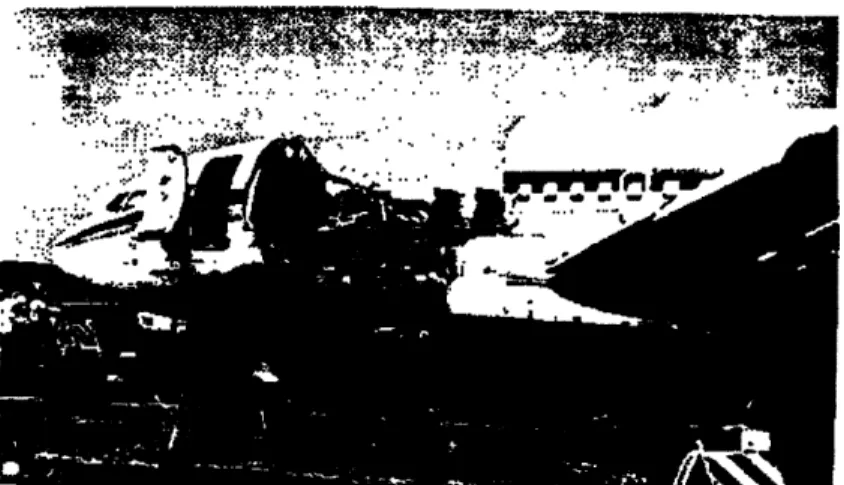
In addition to these economic costs, there are human costs as well. Many workers have been injured or killed due to corrosion weakened steam pipes rupturing, leaking high pressure, high temperature steam into workspaces. These human costs of cor-rosion struck the airline industry on April 28, 1988 when an Aloha Airlines Boeing 737, flight 243, experienced a failure in a joint in the aircraft skin at 24,000 feet[2]. A large section of the aircraft skin was torn away, resulting in rapid decompression of the aircraft cabin. One flight attendant was swept overboard, presumably killed, and eight other individuals were seriously injured. The reason for the failure of the joint was determined to be fatigue cracking of a bonded, riveted joint connecting sections
Figure 3-1: Photograph of Aloha Airlines Flight 243
of the aircraft skin. A similar accident occurred in the Republic of China in 1981, when a 737 experienced a similar explosive decompression of the cabin. The cause of the accident in China was determined to be "extensive corrosion damage in the lower fuselage structures, and at a number of locations there were corrosion penetrated through pits, holes and cracks due to intergranular corrosion and skin thinning exfo-liation corrosion . . . resulting in rapid decompression . . . midair disintegration[1]."
3.2
Corrosion of Aluminum Aircraft Structures
Corrosion is an electrochemical process that damages metal through dissolution of the metal atoms. A metal atom has electrons ripped away from it by another atom which strongly attracts electrons, like oxygen. The metal atom is said to have been oxidized and the atom that receives the electrons is said to have been reduced. Through this process, metal atoms are dissolved as ions in solution, and the metal structure is weakened through material loss.
3.2.1
Corrosion Products
Professor Marcel Pourbaix pioneered a useful technique in corrosion science. He wrote down equilibrium reactions for all possible reactions the metal might undergo when it is oxidized, and determined which reactions were energetically most favorable in certain environments. These are graphically represented as regions of a two dimen-sional diagram where the vertical axis represents the electric potential of the metal vs. a standard cathode and the horizontal axis represents pH. The regions indicate the most stable corrosion product for that environment. Figure 3.2 shows the Pourbaix diagram for aluminum in deaerated water.
From Figure 3.2 one can see that three corrosion products are possible, Al3+ in
solution, A1203 : 3H20, or Al02-. The most common form of corrosion product is
aluminum oxide hydrate, A1203 : 3H20.
3.2.2
Types of Corrosion
There are many different types of corrosion, but they can be divided into two gen-eral categories: uniform attack and localized attack. Uniform attack is characterized by uniform dissolution of material over the entire metal surface. It accounts for the greatest tonnage of material lost every year. [21, p. 11] Localized attack, while ac-counting for much less material loss, is of greater concern than uniform corrosion because it is much harder to predict, detect, and control. Forms of localized attack include pitting, crevice corrosion, intergranular attack, stress corrosion cracking, and corrosion fatigue cracking.
Localized forms of attack tend to have penetration rates much higher than those of uniform corrosion. This is because localized attack allows the local environment to become isolated from the rest of the electrolyte, causing corrosion products to build up and changing the concentrations of ions in the solution. Metal ions in solution
-? '-1 Q 1 2 re 5 7 a 8j orr It I
Figure 3-2: Pourbaix Diagram for Aluminum
r
!
!
Global Environment (pH = 7)
A1(OH)3
Environment
IH < 7)
Figure 3-3: Chemistry of a Corrosive Pit
tend to precipitate out as hydroxides, lowering the pH of the local environment. The buildup of insoluble hydroxides tends to limit diffusion of hydroxide ions from the global environment into the local environment, causing the pH of the isolated en-vironment to drop. This increasing acidity of the local enen-vironment increases the corrosion rate, putting more metal ions into solution, which precipitate out more hydroxide ions, which lowers the pH even more, continuing the cycle. This positive feedback loop accelerates the corrosion process. This effect is most pronounced at the
crack tip, causing the defect to deepen at a faster rate than it widens.
The factors that control this feedback process are the solubility of the metal hy-droxide, the size of the "local" environment, and the rate of diffusion of the ions in solution. Any area that allows a portion of the corrosive electrolyte to be isolated is vulnerable to this type of accelerated local attack. Some examples of vulnerable areas are cracks, scratches, crevices formed from joining two surfaces (as in a lap joint), rivets, and pits formed when corrosion resistant coatings fail locally.
may be deep enough to penetrate the entire thickness of the material. From Figure 3.3 one can see that these localized forms of corrosion will often result in the attacked regions being left packed with corrosion product, either AI(OH)3 or A1203 : 320.
3.3
Non-Destructive Evaluation of Corrosion in
Aircraft Structures
3.3.1
Benefits of NDE to the Airline Industry
The airline industry could save a great deal of money with a fast, inexpensive, reliable non-destructive inspection process to locate corrosion in aluminum structures. This would allow the airlines to catch the corrosion early and repair a small, inexpensive problem rather than a large, costly one. It would also decrease the amount of time each aircraft spent inoperable due to corrosion related problems. Airlines are very concerned with minimizing the amount of time aircraft must spend on the ground, and taking an aircraft out of service in order to repair corrosion damage is a very costly affair even if repair costs are ignored and only revenue lost due to flights not completed is considered. An effective non-destructive inspection procedure would also extend aircraft service life.
3.3.2
Aging Aircraft Concerns
We have already mentioned that it is economically advantageous to the airline in-dustry to extend aircraft lifetimes as long as possible due to the huge capital cost of the aircraft. Twenty years ago this was not an issue of great concern because large, commercial jet aircraft fleet was relatively new. Today, however, some of the aircraft still flying are older than many of their passengers.
User Total Total Over % Over In Fleet 20 Years Old 20 Years Old
Army Helicopters 8,115 5,176 64 Fixed Wing 330 179 54 Navy/Marines Helicopters 1,385 579 42 Fixed Wing 3,129 529 19 Air Force Fixed Wing 4,493 2,560 57 Total Military 17,452 9,087 52 Total Commercial 5,084 1,700 33
Table 3.1: Aging Aircraft Summary
continuously due to economic concerns like civilian aircraft. There is an additional problem, though, in that the military cannot independently determine the service lifetime of its aircraft. An excellent example is the KC-135 mid-air refueling tanker. The aircraft was brought into service in the mid 1950's, and Congress has recently voted to appropriate funds for a replacement aircraft in 2045. The Air Force has no choice but to continue operating the older aircraft past their intended lifetime. This is not an isolated example. A study in 1990 concluded that corrosion damage to U.S. Air Force aging aircraft is the most significant cost burden of any structurally related factors.[11] Table 3.1 shows the average age of various types of aircraft, both military and commercial[9].
3.3.3
Present State of Non-Destructive Inspection of
Air-craft
The airline industry presently relies on two techniques, visual inspection and eddy current probes.[19] Visual inspection is a non-quantitative technique that doesn't al-low for inspection of areas that an operator can't access. It is effective at detecting
more advanced corrosion, but it is difficult to see the early stages of uniform corrosion or localized forms of corrosion, such as small pits and cracks.
The eddy probe monitor is a device that relies on the fact that aluminum con-ducts electricity and the corrosion procon-ducts of aluminum do not. The probe is a small, hand-held device that induce eddy currents in the aircraft skin. The behavior of the eddy currents allows the operator to determine the thickness of the conduc-tor. In this way the amount of material lost to corrosion can be determined. It is an accurate technique when the instrument is handled by an experienced operator and is calibrated correctly. Drawbacks of the eddy current probe are that it is not very effective at detecting localized forms of corrosion attack such as pitting or stress corrosion cracking and that it is a very time consuming technique. Operators must literally crawl over the skin of the aircraft with the probe, which can only test a small area (on the order of square centimeters) at one time.
3.3.4
Neutron Radiography and Detection of Corrosion in
Aircraft Structures
In order to determine if neutron radiography is suitable for imaging corrosion in air-craft structures, one must remember the requirements for radiography. Radiography requires that the radiation penetrates the bulk material and that the details one wishes to image has a high attenuation coefficient.
Table 3.2 shows the elemental cross section for aluminum, oxygen, and hydrogen for soft x-rays (30 keV), thermal neutrons (0.025 eV) and cold neutrons (0.005 eV).
Element X-Rays Thermal Neutrons Cold Neutrons 30 keV .025 eV .005 eV Hydrogen 0.597 38.30 65
Oxygen 9.810 4.20 6.0 Aluminum 49.3 1.42 1.5 Table 3.2: Cross Sections of Various Elements
(10- 24cm2)
different materials by the following formula:
for X-Rays and Neutrons in barns
MWi
S= (jiXiaiAo) p
P (3.1)
Where:
* Ei = sum over all isotope types present in material
* Xi = mole fraction of isotope i
* P = linear attenuation coefficient (cm- 1)
* ai = atomic cross section ( cm) of isotope i
* Ao = Avogadro's Number = 6.02x10231atom
* MWi = molecular weight of material
* p = density 9 of materialCm3
Using equation 3.2, we can determine the linear attenuation coefficients of alu-minum and corrosion products for soft x-rays, thermal and cold neutrons. The results are listed in table 3.3.
Table 3.4 makes it easy to see why thermal neutrons are a better choice for imag-ing corrosion in aluminum than x-rays. Recall from Chapter 2 that the total fluence required to image a detail of fixed size is proportional to the inverse of the square of
Material X-Ray Thermal Neutron Cold Neutrons
30 keV 0.025 eV 0.005 eV
Al 3.0 0.085 0.086
A1203 :3H20 1.57 2.51 4.18
Al(OH)3 1.50 2.41 4.55
Table 3.3: Linear Attenuation Coefficients for Aluminum and Corrosion Products for X-Rays and Neutrons (cm - 1)
Material & vs Aluminum
X-Rays Thermal Neutrons Cold Neutrons
Al 0 0 0
A1203 : 3H20 0.48 2.85 4.76
Al(OH)3 0.50 2.73 5.19
Table 3.4: M for Corrosion Products in Aluminum for Different Radiation Types and cold neutrons than for x-rays, making neutrons a better choice for imaging cor-rosion in aluminum structures.
Chapter
4
Detector Configuration and
Characteristics
The detector used in this work consisted of commercially available elements. No ex-pensive, custom made parts were required. This was an important concern because the purpose of this work is to show that neutron radiography is a practical technique for use in the field. Exotic and delicate materials are not suited for field work. After considering the available detector types, we chose a scintillator coupled to a CCD camera because it is a simple, relatively inexpensive detector with low noise and high spatial resolution.
4.1
Theory of Position Sensitive Neutron
Detec-tion
Direct spatially localized detection of neutrons is a difficult task. Most position sen-sitive neutron detectors rely on a neutron converter, which converts the neutron into a more easily detected secondary radiation, such as a photon, electron, or alpha par-ticle. The detector used actually detects this secondary radiation.
When choosing a converter-detector pair, one must consider a number of factors. Neutron converters must balance efficiency with spatial resolution and output of sec-ondary radiation. One must also match the secsec-ondary radiation produced in the converter to the proper type of detector. By choosing the appropriate balance of these factors, one can maximize the detector response per unit neutron flux.
4.1.1
Gas
Detectors
Gas neutron detectors rely on a gas as a neutron converter. A gas with a high neutron cross section is chosen, such as boron trifluoride (BF3) or helium (He3). An incident
neutron strikes a gas molecule and ionizes it. A high voltage is placed across the gas chamber, accelerating the liberated electron and the ion towards the electrodes. As the particles are accelerated towards the electrodes, they gain energy and collide with other gas molecules, causing additional ionization. In this way a cascade of electrons and positive ions is formed, and a measurable charge is collected at the electrode. This measurable charge is the detector output signal.[10]
These types of detectors have been used in a position sensitive manner in two ways. One method is a discreet element gas detector, which is simply many small gas detectors placed in an array. Because each detector has an individual output, it is easy to determine where the neutron was detected. These detectors are expensive, require many outputs to be monitored, are easily saturated, and have very poor spa-tial resolution. They are not suitable for radiography.
A second gas position sensitive detector is a multiwire gas detector. This is a single gas chamber with a grid of wire electrodes. Because the charge is created and collected in a small area around the neutron interaction site, the electrode nearest the interaction site will collect the most charge. The neutron detection site can be found by using the vertical and horizontal wire with the largest response. These detectors are also expensive, delicate, and have poor spatial resolution, making them unsuitable
for radiography.
4.1.2
Scintillator Methods
Scintillator detectors are materials that have two characteristics. First, they have molecules with high neutron cross sections to absorb the energy of incident neutrons. Second, they have special added molecules that accept energy from nuclei excited by an incident neutron and release that excitation energy as a visible light photon. Thus, scintillators are neutron converters with visible light photons as the secondary radiation. The photons are converted into an output signal using a photomultiplier tube.
Like gas detectors, they have been used in a number of ways as position sensi-tive neutron detectors. Similar to a discreet element gas detector, as discreet element scintillator detector consists of many individual scintillator detectors in an array, each with an individual output. The detectors are expensive and have poor spatial
reso-lution.
The scintillator detector known as the Anger Camera is similar to a multi-wire gas detector. It consists of a single scintillator with many phototubes behind it. The neutron detection site is found by taking a weighted sum of the output signals from the phototubes. These detectors have poor spatial resolution and have problems with being saturated..
4.1.3
Film Methods
Film methods rely on materials with high neutron cross sections that undergo an (n,7) reaction, such as gadolinium. A thin foil is coupled to a photographic emulsion screen. The photons produced in the film are then detected in the photographic plate.
The detector response is measured by the darkening of the photographic plate. These detectors have excellent spatial resolution, but have other problems. One is that the response is not linear with detector flux. This means that the imaging system is not linear, as defined in chapter 2, and cannot be analyzed using the sim-plifications we used for a linear, stationary system.
4.2
Detector Configuration
The detector used for this work consisted of a commercially available scintillator screen whose output was directed and focused onto a charge-coupled device used for imaging purposes. The entire set-up was encased in a light tight aluminum box to prevent noise from external light affecting the detector. This aluminum box was cov-ered with 5.1E-2 cm thick cadmium sheeting on three sides to reduce the number of thermal neutrons that reached the screen after scattering from the sides or above the
detector. The detector is shown in Figure 4.1.
4.3
Scintillator
The scintillator screen used was a Nuclear Enterprises NE-426 screen. It uses lithium flouride with a zinc sulfide actuator. The lithium flouride is enriched in Li6, which has
a very high thermal neutron absorption coefficient of 945 barns. The Li' undergoes an (n, a/) reaction, liberating a 2.05 MeV alpha particle. The energetic alpha particles then collide with zinc sulfide molecules, transferring energy in the collision. These energetic zinc sulfide molecules then relax, emitting visible light photons in order to lose the energy the gained as the result of the collisions with alpha particles.
Scintillator Scree
Lens
lJ1
Figure 4-1: Components of Imaging System
CCD Chip
U
I---~ec--- ·---~--
-hN ]
screen. The first factor is the fraction of incident neutrons that react in the screen. This neutron efficiency is a function of two variables, the thickness of the screen and the density of Li6 in the screen. Spowart investigated the effect of these two factors on the light output of the scintillator screen.[33]
The NE-426 screen used was 0.25 mm. Spowart investigated screens of thicknesses from 0.05 mm to 1mm and found that the optimal thickness for radiography was 0.25 mm. The thickness could be increased in order to increase the neutron efficiency, but at the expense of both light output and spatial resolution. Light output for a thicker screen is slightly lower due to self absorption and spatial resolution is decreased. Screens thinner than 0.25 mm had problems due to non-uniform distribution if the lithium flouride.
The NE-426 screen used has approximately 15% neutron efficiency. It has one part lithium flouride and four parts zinc sulfide by weight. We chose this value because Spowart investigated the light output of scintillator screens with ZnS/Li6 weight ratios from about 0.1 to 6 and found that the peak light output is obtained for a ZnS/Li6 weight ratio of four. The light output measured by Spowart for this screen was 1.7x10⁵ photons per detected neutron. Because photon from the screen is isotropic, only half of these photons, or 8.5E4 photons per detected neutron, were produced in a direction such that they were directed onto the CCD camera.
4.4
Camera
The camera used to image the scintillator screen was a Princeton Instruments TE/CCD-1242E. The CCD is an EEV 05-30 with 1242x1152 pixels. The chip size is 28 mm x 26 mm, for a pixel size of 22.5 pm x 22.5 im. The camera is interfaced via a Princeton Instruments ST-138 controller which can be read out at high speed (12 bits, 1 Mhz) or low speed (15 bits, 430 kHz). The ST-138 also controls the thermoelectric camera
1 0.8- 0.6- 0.4- 0.2- 0-0 10 20 30 40 50 60
PHOTON ENERGY [keV)
Figure 4-2: CCD Efficiency vs Photon Energy
cooling mechanism, which can be run air cooled or with circulating chilled water.
4.4.1
Efficiency of CCD
The photon efficiency of the CCD depends on the photon energy. Koch measured the efficiency of the CCD vs photon energy and found that the peak efficiency was about 30% at photon wavelengths of 550 nm (See Figure 4.2). [24] Because the NE-426 photon emission spectrum has it's peak below this wavelength, copper (Cu) was added to the scintillator to shift the peak emission towards the area of highest CCD efficiency. The efficiency changes relatively slowly with photon energy, however, so we assumed a total efficiency of approximately 30%.[27]
4.4.2
CCD
Noise Characteristics
The noise characteristics of CCD detectors have been investigated by Schempp and Toker.[28] They determined the noise in the CCD signal comes from three sources: background photon noise, dark current, and readout noise. The total noise is given by the following expression:
-DQE
o DQE.measured
.. .... ... ... ....
/(P + B)tQe + Dt + Nr2
where:
* P = signal photon flux * B = background photon flux
* t = integration time
* Qe = detector efficiency
* D = dark current
* Nr = readout noise
Background Noise
The first source, background photon noise, is easy to understand. It is fluctuations produced in the CCD output due to the statistical variation in background photon flux. Because our detector is in a light tight box, there is no visible light background radiation. There is, however, background radiation in the form of x-rays and gamma rays produced by the accelerator itself and in the beryllium target used for neutron production.
In order to determine the effects of this x-ray flux, we exposed the system to iden-tical neutron fluxes in two situations; first the camera was left bare and the mean pixel response was measured. Then camera was surrounded by lead bricks two inches thick and the measurement was repeated. After each measurement of camera response, the neutron flux was measured using a GS-20 thermal neutron scintillator, which is a glass scintillator that also uses the Li6 thermal neutron reaction to detect neutrons. This GS-20 response was used to normalize the CCD response, as the neutron production rate may vary slightly even with the same accelerator settings. The following table contains the raw data collected. Each pixel in the image represents a square in real
Time (m) Mean Pixel Level (ADC Counts)
9.1 uAwPb 9.1uAw/oPb 40uAwPb 40uAw/oPb .5 127.07 170.00 231.02 406.56 5 621.78 1045.40 1683.60 3360.89 10 1172.67 2003.64 3299.82 6674.59 20 2271.47 3947.58 6569.02 13434.03 30 3364.62 - 9885.27 20133.15 GS-20 Counts Over 5 m 56275 52123 281319 284023
Table 4.1: Average Pixel Exposure, Shielded and Unshielded CCD space 1.6E-2 cm on each side.
The data from the previous table is contained in the following two plots. The horizontal axis represents the time of exposure and the vertical axis represents the mean pixel value divided by the number of counts per second measured by the GS-20 detector. This was done to normalize the values for slight fluctuations in neutron flux. It is easy to see from these plots that the CCD is sensitive to the x-ray flux pro-duced in the accelerator and target, but this background noise can be controlled by placing lead around the CCD camera. It is difficult to generate a specific numerical value for B because the x-ray flux produced depend on the accelerator settings and current. Thus, B is different for different accelerator settings and current. To reduce this x-ray contribution to the background level, B, the CCD was surrounded on all sides by 2" of lead. Additionally, We placed a .25" thick lead sheet at the base of the cement brick and polyethylene moderator structure surrounding the neutron source.
We did not generate a spectrum of the x-rays and gamma rays that might cause this background noise in the CCD. The specifics of the photon spectrum were of no concern to us, we simply wanted to know if the detector performance was improved by shielding the CCD with lead, and the data above shows that convincingly.
9.1 uA Average Current, Comparison of Detector Response with and without Pb
0 5 10 15 20 25
Time (s)
+ = without Pb
X = with Pb
Figure 4-3: Mean Pixel Level, Shielded and Unshielded CCD, 9.1 uA Beam Current
'-2 o o a) C, 0 C
--41 uA Average Current, Comparison of Detector Response with and without Pb
0 5 10 15 20 25
Time (s)
+
= without PbX = with Pb
Figure 4-4: Mean Pixel Level, Shielded and Unshielded CCD, 40.0 uA Beam Current
25 g20 0 co a) 0 : 15 O o•0 0 C w) .e
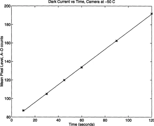
Time (s) Mean Pixel Level (A-D counts) Std. Dev. (A-D counts) 10 87.12 2.33 30 104.92 5.02 45 119.79 7.24 60 133.53 9.47 90 162.38 13.96 120 191.93 18.52
Table 4.2: Dark Current Data
Dark Current Noise
Understanding the second and third noise sources requires a very basic understand-ing of how CCD detectors operate. They can be thought of as a grid of capacitive wells that trap electrons liberated as a photon passes through the semiconductor chip, exciting electrons into the conduction band. These "wells" are then read out sequen-tially. Dark current noise that part of the output signal that is due to electrons that are thermally excited into the conduction band and then collected in a capacitive well. It obviously depends on the temperature of the CCD chip. for this reason, we kept the CCD chip cooled to -50 degrees Celsius with a water cooled thermoelectric Peltier device.
We measured the dark current noise by taking exposures for different times and measuring the mean pixel level. The results are shown in the table and plot below.
The dark current is equivalent to the slope of this curve, which is 0.9547 ADC per second per pixel. An ADC is an analog to digital count, and is simply a measurement of the number of electrons collected per pixel "well".
Readout Noise
The readout noise is caused by the method of reading each pixel "well" out the the ST-138 controller. The contents of each "well" are transferred from pixel to pixel
Dark Current vs Time, Camera at -50 C
0 Time (seconds)
Figure 4-5: Dark Current Exposure vs. Time
as successive pixel "wells" are read out. This process can be thought of as a bucket brigade, where the contents of each bucket are poured into the next as the final bucket is emptied (i.e. read out). The readout noise is the variation in the signal produced due to this transfer process. Because this noise is a factor of the way the CCD is read out and not any factors depending on time, it is independent of time. In the plot above, the readout noise can be found from extrapolating the data back to time zero and finding the ADC level. The readout noise for our system is 76.7906 ADC per pixel.
Fixed Pattern Noise
Fixed pattern noise is noise that is introduced into the signal due to imperfections in the CCD chip itself. These imperfections occur at a fixed location on the CCD chip, hence the name fixed pattern noise. Fixed pattern noise does not occur in the equation for CCD noise because it is very easy to eliminate. It can be eliminated
r-o a C = 0I .-J a,