339
Determining Shear Wave Velocities in Soft Marine
Sediments
by
J .A. Meredith, C.H. Cheng and R.H; Wilkens
Earth Resources Laboratory
Department of Earth, Atmospheric, and Planetary Sciences Massachusetts Institute of Technology
Cambridge, MA 02139
ABSTRACT
The inversion technique presented in this volume (Cheng, 1987) that simultaneously inverts full waveform acoustic logs for shear wave velocity
(Va)
and compressional wave attenuation(Qp)
was applied to selected full waveform acoustic logs taken in soft sedi-ments from Deep Sea Drilling Project Site 613.Besides V. and
Qp,
the sensitivity of the inversion to perturbations in the fixed parameters, P-wave velocity(V
p ) , fluid velocity(V,),
borehole diameter, bulk density(Pb) , and borehole fluid attenuation
(Q
I), were tested. Our study shows that the inversion technique is most sensitive to the estimate ofVp because the inversion is basedon the P leaky mode energy portion of the spectrum. The Poisson's ratio, however, which primarily controls the amplitude of the waveforms, is rather stable with different estimates in Vp • The inversion technique is less sensitive to small perturbations in
borehole diameter, Pb, VI> and Q"
The shear wave velocities inferred from these inversions correlate well with the at-tendant velocity logs run at Site 613 and the diagenetic changes identified by shipboard stratigraphers. For example, there is an increase in both Vp and V. at the diagenetic
boundary between siliceous nannofossil oozes and porcellanite. This boundary is respon-sible for a sharp seismic reflector in a USGS. seismic line run nearby. Over the depth interval that we analyzed, from 390.0 to 582.0 meters below sea floor, we determined shear wave velocities ranging from 0.74 to 1.06 km/sec corresponding to compressional
V.
=
wave velocities from 1.70 to 2.20 km/sec.INTRODUCTION
A goal long sought after by both the exploration geophysics and ocean engineering com-munities has been the determination of shear wave velocities in soft marine sediments (Hamilton, 1976). For ocean engineers, interest-lies in determining slope stabilities and strength parameters for underwater construction, plus being able to calculate acoustic wave propagation properties at the ocean-sea floor interface. For marine geophysicists, the primary motivation to study shear wave velocities is to help delineate reflecting horizons and diagenetic boundaries.
Despite this interest, determining shear wave velocities in soft marine sediments has been difficult and until recently no measurements with velocity or full waveform acoustic logs had been run. Inside the laboratory, as Nafe and Drake (1957) and Hamilton (1976) pointed out, indirect measurementsofV.can be made by first determining bulk modulus
(x:)
andVp experimentally and then determiningV. using the following equation_3(pV/ -
x:)
4pA similar equation was developed by Nafe and Drake for an empirical shear wave velocity-porosity relationship.
Of the few direct laboratory measurements ofV. in unconsolidated marine sediments, those of Kim et al. (1985) and Kim et al. (1983) are most relevant. They determined shear wave velocities from Western Pacific DSDP cores and conducted their shear wave determination at atmospheric pressure. In both studies, they examined sediments more deeply buried than the sediments Site 613 penetrated but one value at 383.0 meters is available for comparison. We will compare this measurement and one reported by Hamilton (1976) in the Results section of this paper.
Hamilton(1976) presented some novel techniques to compute shear wave velocities in situ. One interesting technique is to measure Stoneley waves at the surface from deep submersibles. Measurement of Rayleigh wave phase velocities determines a shear wave velocity but this measurement must be averaged over the volume of sediment the Rayleigh wave penetrates. Shotpoint surveys and VSPs have also been used but are affected by the highly attenuating nature of the unconsolidated sediments. Along with cross borehole measurements, these determinations have been limited to 140 meters depth and higher (Hamilton, 1976).
Seismic refraction and wide angle reflection surveys have also been made but suffer
Shear Waves In Marine Sediments 341
the same resolution problem of averaging over large volumes. Much recent interest has centered around developing direct she?-r wave logs. A tool presented in Zemanek et al. (1984) has been tested in soft marine sands but results are not yet available for
comparison.
The shear wave velocity of soft marine sediments is less than the acoustic velocity of the drilling fluid inside the borehole. Specifically, the slower formation shear wave velocity causes any potential refracted shear head wave to not reach the critical angle necessary for refraction. Thus any potential shear head wave gets refracted into the formation instead of the borehole. So traditional methods that rely on picking the shear dominated pseudo-Rayleigh wave, for instance (Willis and Toksaz, 1983), simply do not work.
Many investigators (White; 1965, Cheng and Toksaz; 1983; Chen and Willen; 1984, Stevens and Day, 1986) have investigated determining shear wave velocities in soft sediments by inverting the dispersion relation for the Stoneley wave present in low frequency full waveform logs. However, there are difficulties with this procedure which warrant developing other techniques. First, as pointed out by Paillet and Cheng (1986), the Stoneley wave becomes undetectable above 5 kHz for soft marine sediments, thus mandating low frequency or very broad band tools. Second, inverting for shear wave velocities based exclusively on the Stoneley wave velocity neglects high permeability at the fluid-borehole interface which affects Stoneley wave propagation (Rosenbaum, 1974; Williams et aI., 1984). As pointed out by Cheng and Toksaz (1983), the sensitivity of Stoneley wave velocity to shear wave velocity is not very great, so high quality data is needed. The algorithm presented in Stevens and Day (1986) additionally inverts for Vp ,
Pb, VI' PI and tool radius for a total of six parameters. This large number of parameters can cause too much variation to be attributed to parameters that can justifiably be fixed. Because of these factors, we decided a proper indirect inversion for shear wave ve-locities in soft marine sediments should take attenuation into account and should have demonstrated utility for any frequency band data available. We are confident that the borehole and fluid parameters are sufficiently well known to justify a two parameter in-version, the parameters being V. and Qp. By taking the inversion based on the P leaky mode wavetrain, most common full waveform logs can be used for the inversion process, and the adverse effects of excessively high or low permeability on the pseudo-Rayleigh and Stoneley waves are negated.
DATA DESCRIPTION
DSDP Site 613 was drilled during Leg 95 of the Deep Sea Drilling Project in 2333 meters of water. Both USGS seismic line 25 and the Continental Offshore Stratigraphic Test
wells B-2 and B-3 (COST B-2, COST B-3) investigated the Baltimore Canyon Trough area near Site 613. Site 613 is located at. the southern edge of the Baltimore Canyon trough, 250 miles from the New Jersey coast on the continental slope and represents a deep sea, pelagic, sedimentation environment.
Wilkens et al. (1986), and Goldberg et al. (1985) describe the stratigraphy, phys-ical properties, and analysis of the velocity, gamma ray, and resistivity logs in detail for Site 613. An important observation made in those papers is the high porosity of the sediments; porosities vary from 40 to 70% . Generally, beyond the initial terrige-nous components, the sediments are comprised of pelagic carbonaceous and siliceous nannofossil oozes. There is a gradual carbonate pelagic ooze to chalk transition which takes place over hundreds of meters. In only a few meters, the siliceous components go through an abrupt transition from almost pure opalline nannofossils to a porcellanite framework (Calvert; 1974, Wilkens et al.; 1985, Goldberg et aI., 1985) and can be seen in scanning electron microscope images (Wilkens et aI., 1985).
Specifically, at Site 613, the stratigraphic profile is divided into three units. First, there is a layer of primarily pelagic terrigenous sediments 280 meters in thickness under-lain by a transition to more homogeneous siliceous nannofossil ooze. This layer ranges from Upper Pliocene to Middle Miocene in age and can be seen as Unit I in Figure 1. Unit I contains clays, which have more radiogenic elements than the nannofossil oozes, resulting in a dramatic decrease in gamma ray count at the Unit I-Unit II boundary. TheVp and formation factor log also show this boundary but not as dramatically. Unit
II ranges in age from Middle Eocene to Lower Eocene. At about 440 meters below sea floor depth, an abrupt transition from Unit II to Unit III occurs which represents the diagenetic change in the siliceous component from ooze to porcellanite. A portion of full waveform logs from this transition zone is displayed in Figure 2. In this transition zone, there is an increase in both compressional and shear wave velocities. Moreover, there is also a decrease in porosity from between 50 to 60% down to 40%. The difference between Unit II and Unit III is primarily a physical one; the chemical compositions are very similar. The boundary between Unit II and Unit III correlates well with a reflector identified in USGS seismic line 25. Unit III is Lower Eocene to Maestrichtian (Creta-ceous) in age. The gamma ray log stabilizes below 520 meters and the formation factor andVp adopt a considerably gentler gradient. We believe this gentle gradient is related
to increased lithification in the ooze to chalk transition and increased compaction due to greater depths. The drilling terminated at about 580 meters depth in Unit III.
FORWARD MODEL
The forward model is a pressure response integral calculated around singularities in the complex wavenumber domain. Three available methods to calculate this integral include
Shear Waves InMarine Sediments 343
1.4
Vp
(km/sec)
1.8
2.
F
GAMMA
(gapi)
o
LITH
UNIT~u.
Plol.tocet
II
I
III
L. EocetM L. EocetMu.-u.
MIocen
M.Eocene
":::··::.··::·::::·:r:::::.::.
.. •.••...,! ~ . ...! ~ . . , ~..···j"···T·
···i···~..··· : : ...} ! ,!, ~ ,- . : ; ....···7···..· ...~ -: •···f···..··J··..
....
~l8:
.
, ···f···i···~· ....·· ..·i... ...;
.
...~ ....
~ ....
:.
...c . ···i··· . ..;.
···r···
.
~...
~...
...
":' .....····+....
····1··..·
: :...
.:..
••••••• t" •••••••••~••••••••• ···~···t·....····
: : ~ ! ~ . ~···~···r·..···
····1..
···t..··..···t····..··
; ; ;···..
·.;.···~···r····..···.;.···
! :
i :
...,.
(.
: : i ;: :...
~
...+...
....···1···..····
...
.; ....
".···..1···
···1···...,
40
120
440
200
360
520
280
-; ..
J:
I-Q. WC
...
E
TIME
(M U)
~
10
10.00
51.20
102.40
153.60
2 4.80
256.00
0 I I r11 .s=.s= LJ <.a --j.
:::r:
0 0 ~ 3: r11 --j r11.s=:rJU1
(J):"
- en).00
51.20
102.40
153.60
204.80
256.00
0TIME
(MU)
~
1 0
1RECEIVER -I
Shear Waves In Marine Sediments 345
real&Xisintegration (Rosenbaum, 1974), branch cut integration (Peterson, 1974; Tsang
and Rader, 1979) and a ray expansion of the kernel in the branch cut integration (Tsang and Rader, 1979). We chose the branch cut integral method of Tsang and Rader and the method is fully described in the preceding paper (Cheng, this volume).
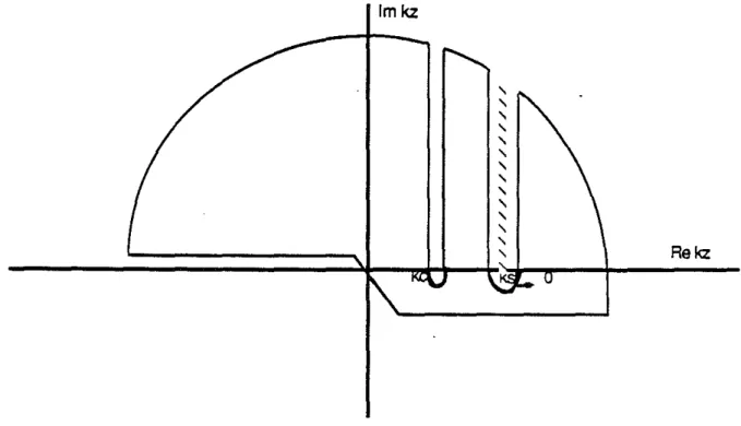
The first step consists of calculating a steepest descent branch cut integral around the compressional branch point on the real wavenumber axis k
=
k,. A map of the singularities in the complex wavenumber domain and the contour integral is highlighted in Figure 3. Although the method is in general applicable to both hard as well asImkz
,,
,,
,,
,
,,
,,
,
,,
RekzFigure 3: Wavenumber plot showing branch points
soft sediments, particular simplifications occur when soft sediments are considered. For example, since the shear head wave does not propagate in soft sediments the branch cut integral around the shear head wave can be neglected along with the pseudo-Rayleigh wave pole. Furthermore, at the relatively high frequencies of the Schlumberger tool, the Stoneley wave isnot excited. Thus the pressure response simplifies to minusthe branch cut integral and no prewindowing of the waveform to isolate the P wave is required.
This branch cut integral is computed with the standard assumptions of an axially symmetric, fluid-filled borehole with an infinite homogeneous formation surrounding it. Furthermore, point sources and receivers are assumed with no tool present. The
integral is evaluated using numerical quadrature. For this study we chose 4th order Gaussian-Laguerre quadrature after investigating up to tenth order quadrature. For our purposes, it is sufficient to calculate the frequency integral because the inversion calculations will all be done in the frequency domain. Attenuations are introduced by assuming complex velocities and thus complex wavenumbers.
In Cheng et al. (1986), we discussed forward models of soft sediment full waveform acoustic logs using the discrete wavenumber representation (Bouchon and Aki, 1977; Schmitt et aI., 1985). The discrete wavenumber representation computes all arrivals simultaneously including both head waves and guided waves. In that study, a Kelly source at a center frequency of 12 kHz (Kelly et aI., 1976) was used and parameter vari-ations studied included Poisson's ratio
(0"),
Pb, Qp and Q3' We concluded that Q3 has a negligible effect on soft sediment full waveform logs because of the absence of a shear head wave arrival and also showed that a reasonable range of bulk density variation does not significantly affect the waveforms. However, Poisson's ratio strongly affected the amplitude of the leaky P mode (Cheng and Toksoz, 1981) andQp also had a visually discernible effect. In this study, although only the compressional branch cut contribu-tion is calculated, the same conclusions apply as shown below in the inversion seccontribu-tion. Additionally, variations in tool radius, Qt, and fluid density are also investigated for the inversion procedure and are shown to be important.INVERSION PROCEDURE
To accomplish the inversions, we first calculated .two 512 pt. FFTs of data at two successive source-receiver separations and then computed the direct spectral ratio. In the soft sediment case, windowing of the waveform prior to taking the FFTs is not necessary because the waveform is mostly P wave energy and we are inverting the P wavetrain. Another simplification occurs because the full waveform log is a real valued time series, so the FFT is conjugate symmetric and only half of the FFT is required to calculate the spectral ratio (Oppenheim and Schafer, 1975). After computing the spectral ratio, the branch cut integral of the compressional branch pointkc is evaluated
for the two source-receiver spacings and the forward model spectral ratio is calculated. By taking the spectral ratio, the problem of unknown source function can be neglected. The spectrum is then windowed to exclude the low energy side lobes which cause undue noise in the spectral ratio. The spectral ratio for the inversions done in this study was windowed between 7.5 and 15 kHz.
The windowed spectra are inversely weighted with frequency so that all the frequen-cies are equally emphasized in the inversion. Finally, the data spectral ratio and forward model spectral ratio are compared in a nonlinear iterative inversion. Finite differences are used to approximate analytic partial derivatives and the Cholesky factorization is
Shear Waves In Marine Sediments 347
applisd in evaluating the resolution matrices. The inversion for V, and
Q
p is carriedout simultaneously and the effects of varying estimates of the fixed parameters in the inversion are discussed below.
Parameter Variations
Variations in VpWe used both Schlumberger's threshold detection algorithm and a statistical P-wave on-set program based on the Willis and Toksoz (1983) method to determine compressional wave velocities.
Schlumberger's threshold detection technique relies on the first arrival eclipsing a threshold at successive receivers and works well for high Q formations but often misses low amplitude first arrivals for low Q formations. This is because for low Q (highly attenuating) formations, amplitudes of the first arrivals at successive source receiver spacings might not exceed the threshold and thus cycle skip. Or more commonly, the threshold will be exceeded on different portions of the Bank of the incoming P wave for the two waveforms. This is illustrated below (Figure 4) and results in a consistently slower P·wave velocity determination.
•
-,
+---~~\IFigure 4: Illustration of Schlumberger's threshold detecting technique
The Willis and Toksoz (1983), however, is not based solely on threshold detection but instead measures the onset of the P-wave arrival energy through a semblance correlation following a rudimentary threshold detection. The slowness correlation value allied to
...
-.
>I!J't
*
~
•
C. F. I J----.ti--a be",' ICJlI ST'[P 2:. , ~
R2 "..,..
"
..
...
~ *~•
C.F2~ a , be" taQ STEP '3:Figure 5: lllustration of Willis and ToksOz(1983) method of velocity determination
the highest resulting energy is then chosen as formation compressional slowness. For highly attenuating formations, this technique gives more accurate velocity estimates. (See Figure 5 for a demonstration of the method and Figure 6 for a plot of Willis and ToksOZ picked values versus Schlumberger derived values). As can be clearly seen, there is approximately a 3% to 10% discrepancy between Schlumberger threshold detection derived values versus Willis and Toksaz values, with Schlumberger values being consistently on the low side. We used the Willis and ToksOz values in our inversions and verified them by hand picking first arrivals on some of the logs.
Variations in the initial estimate ofVp do affect the inversion procedure and since the
inversion is primarily based on calculating energy in the leaky P mode, the effects are often significant. Some of the effects relevant to incorrect estimates of Vp are illustrated
in the table below where estimates of Vp from 1.72 km/sec to 2.30 km/sec are given as
input to the inversion. This example is taken from a depth of 447 m and the correct Vpis
believed to be 2.03 km/sec. As can be seen, an initial estimate ofVp that is too low will
often yield an inversion for shear wave velocity that is also too low, essentially preserving the Poisson's ratio. This is true above, especially for P wave estimates between 1.91 and 2.30 km/sec. Poisson's ratio primarily controls the relative amplitude of the leaky P mode so is a more robust parameter in a spectral ratio inversion (Cheng et al., 1986). Another phenomenon observed with incorrect estimates of Vp is that the convergence properties of the inversion change. Instead of sharp minima, the minima are smoothed out as is clearly shown by graphical sensitivity analyses. The sensitivity analyses are calculated by running many different forward models with a matrix of Qp and V. val-ues, comparing the resultant forward model to the data spectrum, and determining an absolute error. Finally, a three dimensional plotting program plots the absolute error at
'Shear Waves In Marine Sediments 349
•
•
•
•
425 500 575
De~th below sea floor (rn)
Figure 6: Comparison of two velocity picking methods
Table 1: Results of inversions for varying initial estimate ofVp , data from a depth of
447 meters below sea floor
Poisson's Vp initial V. Qp Error
Ratio .394 1.72 0.720 22 3.30e-6 .401 1.82 0.741 22 2.80e-6 .370 1.91 0.866 24 1.68e-6 .365 1.97 0.907 21 1.63e-6 .364 2.03 0.940 23 1.37e-6 .362 2.12 0.987 24 1.34e-6 .378 2.30 1.020 23 2.30e-6
each matrix value, creating an error surface. A typical sensitivity analysis is indicated in Figure 7 followed by a sensitivity ~nalysis for the same waveform based on what we believe is an incorrect velocity. As is shown in this figure, in addition to the error being almost an order of magnitude greater, the trend to the surface is much smoother mak-ing determination of a global minimum more difficult. When such a characteristic fiat minima surface was encountered during an inversion or if the inversion did not converge to any kind of minima, this would provide a strong indication that the initial estimate of P-wave velocity might be incorrect. By critically examining theVp value at this depth,
and comparing it toVp values at adjacent depths, it was often found that a determined
valueofVpwas improper. Going back and correcting the value often resulted in a better
inversion with clearly defined global minimum.
Variations inFluid Velocity
A fluid velocity near that of sea water, approximately 1.5 km/sec, was used for the inversions, but we investigated variations up to 1.75 km/sec. Figure 8 shows four sensisitivity analysis snapshots for a fixed Vp and it can be seen that although the
minima are slightly shifted the picked shear wave velocities and the character of the error surface are almost equivalent. This is an encouraging result because we have very little control on the mud velocity in downhole conditions. Particularly with soft sediments, we would expect the drilling fluid to be contaminated by borehole washout.
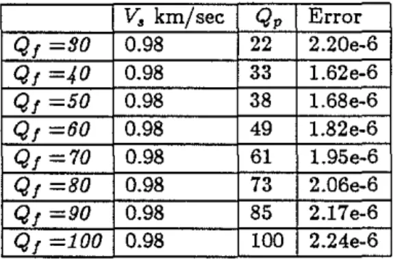
Va.riations in Qf
We used a Qf of 50 in our inversions. The table below shows the results of calculating sensitivity analyses for varyingQf. By changingQf, the result of the sensitivity analyses for
V.
was not affected but asQf increases so does the estimate forQp . As Qf increases from 30 to 100, Qp increases from 22 to 100. The approximate Qf of sea water is 100 so by taking into account borehole washout and drilling mud effects we felt a Qf of 50 was justified. Recent work performed at ERL (Tang et aI., 1987, this volume) indicates that the Qf of drilling fluid may be as low as 30.Borehole Radius Variations
In a soft sediment environment, the potential for washout or borehole collapse is great because of the high porosity, low viscosity nature of the sediments. Therefore, a caliper log is important. It is worthwhile considering the effect of borehole radius variations on the in version results. We systematically varied the borehole diameter and performed
Shear Waves
InMarine Sediments
Vp - 2.1S k/ ••e 351 j I .6 10I
I .6Vs
Vp - 2.30 k/ue II
I 1.1 II '
1.1...
o...
...
w
I I I I I I I I I I I I I I I I I I I I I I I I I I I I I 1 I i I I I I 1 I I I i I 9.6 9.7 9.6 9.9 1.9 I. I 1.2 1.3 I 1 1I I 9.7 9.6 9.0 1.9
I.'
1.2 1.3 1.6 V. V. VI - 1.55 VI - 1.10 ( ( 7 j I I 0.8 I I i t I I I I 0.9 I.IIl V. i i i 1.1 I I i I 2 i ! 1.3 0.6I I I I i0.7 [ , I 0.8 V. i , i 9 9 I I I. 1.9 I I I I. I i I 1.2Shear Waves In Marine SediInents 353
Table 2: Results of varying initial estimate of Q! , data from a depth of 438 meters
below sea floor
V, km/sec Qp Error Q! =90 0.98 22 2.20e-6 Q! -40 0.98 33 1.62e-6 Q! =50 0.98 38 1.68e-6 Q! -60 0.98 49 1.82e-6 Q! -70 0.98 61 1.95e-6 Q! -80 0.98 73 2.06e-6 Q! -90 0.98 85 2.17e-6 Q! -100 0.98 100 2.24e-6
inversions for a waveform at a depth of 451 meters below the sea floor. The results are shown in the table below. Changes in borehole radius do not substantially effect the inversions for V, but these changes do vary the output attenuation values. For the 9.0 em borehole, Qp reaches 80 while it is near 30 for the 10.0 em and 11.0 em radius
boreholes. Absolute errors are about the same for each of the three cases. Table 3: Results of inversions for varying borehole radius
Radius Error em V, Qp 8.0 em 2.2006 0.88 35 9.0 em 2.2006 0.88 83 9.5 em 1.5006 0.87 32 10.0 em 1.7e-6 0.88 31 10.5 em 2.3006 0.87 28 11.0 em 2.2e-6 0.87 30
Bulk Density Variations
A similar analysis to that performed for borehole diameter variations was carried out for a range of density variations. The results are shown in the table below. As can be seen from the table, these large variations in bulk density do perturb the inversion results. Increasing the density by 12% results in a 3% change in output shear wave velocity. Changes in density seem to have no effect on Qp values but this awaits further
observation. Through the use of density logs, accurate estimates of bulk density will be available but unfortunately no such log was available for Site 613. For the inversion
results in this study, based on core measurements, we used a bulk density of 2.0 grams per cubic centimeter as an approximate median bulk density.
Table 4: Results of varying inversions for bulk density, data from a depth of 451 meters Pb-1.75 Pb- 2.OO pb-2 .25
Starting Error 8.060-6 2.600-6 7.830-6
Ending Error 4.440-6 1.700-6 5.700-6
Final Vs .95 .98 1.01
Final Qp 23 20 19
ANALYSIS OF VARIATIONS IN
V,AND
QpThere were two ways of gauging error in the determinations ofV, andQp, relative error and absolute error. Absolute error is a measurement in the frequency domain which represents the square of the magnitude difference between the forward modeled spectral ratio and the data spectral ratio. It is furthermore weighted towards lower frequencies by dividing by the square of the frequency. Absolute error for the V, determined by this technique ranged from 1e-7 to 10-4 and the most stable best fitting inversions were those that generally had the smallest absolute error.
Another important criteria was the relative error. For instance, many times the absolute error was low for all ·of the sensitivity analyses but the differences were so small it was difficult to pick a global minimum. If there was large absolute error but a big contrast between minima and the surrounding values, then convergence was rapid and choosing a global minimum was simple. This is best illustrated in Figure 9.
In the determination of V" it was often necessary to use physical insight in addition to the lowest absolute error to determine the most suitable inversion. For instance, we know from the equations below relating the Lame parameters to the compressional and shear wave velocities that the highest possible shear wave velocity is the compressional wave velocity divided by the square root of two and occurs when A
=
o.
V,=v;
Shear Waves In Marine Sediments
high .rror
good contrast
355I
I 0.7( I
I0.8
II
I0.9
II
i 1.0 II
I 1 . t II
I 1.2low error
poorly defined minimum
I
I0.6
i i i 0.7I
I i '0.8
I
I I I0.9
iI
I I I 1.0I
I I . I II
1.2When). = 0 this corresponds to a Poisson's ratio of zero because (j = (X:2~)' So ( j = 0 provides an upper bound on the determination of shear wave velocity. On the
other hand, when an inversion for V, initially tended toward lower shear wave velocities, there were usually very broad, poorly constrained minima. Therefore, the inversion would proceed to shear wave velocities that would be physically unrealistic according to the few published laboratory studies done, essentially near zero (Nafe and Drake, 1957; Hamilton, 1976; and Kim et a!., 1983). By starting at a different initial estimate ofV, usually higher, in most cases the inversion would converge to a more constrained, even global minimum.
The inversion technique is less sensitive to Qp and the sensitivity toQp is somewhat unpredictable. The Qs are introduced in the model through the denominator of a complex velocity as follows.
tI~
=
(1
+
i/2Qk)
*
Uk
k=
p,s,jBecause Qp is introduced in the denominator, large absolute values ofQp often implied strange behavior. For instance, theQp parameter determined .in the inversion is a delta Qpvalue. Ifthis correction applied toQpwas too large, even negativeQp values could be calculated. The infrequent determinations of negative Qp's almost never occurred until there were such large positive values ofQp, typically larger than 200, that the correction for Qp would overcorrect yielding negativeQp values. In almost no cases did we obtain a stable inversion for V, with a negative Qp, in fact, a negative Qp usually meant the solution was highly oscillatory inbothV, and Qp. Upon encountering negative Qp, the best strategy was to start the inversion procedure over with new estimates ofV, and Qp.
The same discussion also applies to very large values ofQp even when the solution did not oscillate to negative Qp values. Namely, large Qp values implied oscillatory, unpredictable behavior and a strong suggestion to reexamine the data.
Pitfalls - Restrictions on Input Parameters
Inherent in any nonlinear inversion technique are pitfalls to avoid. Obviously, the better the initial estimates of the parameters, the better the inversion so density, caliper logs and measurements of borehole fluid properties are required. The inversion technique is not amenable to a one pass inversion because of its susceptibility to getting trapped in a local minimum. Usually two or three inversions based on a different initial estimate of shear wave velocity will result in a clearly defined minimum.
To avoid being prematurely trapped in local minima, two different step sizes for the finite difference approximation to the partial derivatives were used. When only
Shear Waves
In
Marine Sediments 357an approximate value ofV, was known, a larger step size of 1.2% was used to span more potential parameter space. But when a better estimate of shear wave velocity was available, for instance by determinations in an adjacent interval, a step size of .5% was found to be sufficient and more accurate. The disadvantage to large step size is the potential to skip over narrow global minima.
RESULTS
A physical properties profile including shear wave velocity, Qp dynamic moduli and porosity is presented in Figure 10. At the time this report was written we were still acquiring some portions of Site 613 full waveform acoustic log data. The data presented here represent depths from 390 to 560 meters below the sea floor.
Above the diagenetic boundary (440 m below sea floor), the compressional wave velocities are less than 2.0 km/sec and the shear wave velocities vary between .75 and .85 km/sec. In the transition zone between 440 and 460 mbsf,V, andVpshow a much greater variability of between 0.75 and 1.05 km/sec and 1.7 km/sec to 2.1 km/sec. Below the transition zone, at 460 m and beyond, both the compressional and shear wave velocities stabilize to about 2.1 km/sec and .95 to 1.05 km/sec respectively. The frequency of shear wave velocity determinations here was reduced because of the general uniformity of the ful! waveform logs and determined shear wave velocities at these depths. The stability in the full waveform logs below the transition zone was also recognized in the resistivity, velocity and gamma ray logs shown previously (Figure 1).
A possible indicator of cementation is the segregation of shear wave determinations with different Vp / V, ratios. Figure 11 shows this separation and we believe for the
values ofVp / V, less than 2.25, the Poisson's ratio is decreasing, suggesting better
cementation. On the bottom of Figure 10 can be seen that as V, increases for any depth, Vp does not increase proportionally as much, thus lowering the Vp / V, ratio. Although speculative at this point, this indicates that V, could be a more sensitive indicator of lithology changes than Vp •
Above the diagenetic boundary, Qp is highly variable spanning from 100 to 20 but below the boundary, Qp tapered down to near 20. In general, this gives a profile of Qp decreasing with depth, an observation also noted by Goldberg et al. (1985).
Both shear wave and compressional wave velocities are increasing with depth as porosity decreases and the framework stiffens. A crude straight line gradient fit to the data in Figure 10 following Hamilton (1976) gives a shear wave velocity gradient of approximately .98 sec-1 to be contrasted to Hamilton's value of .58 sec-1 for depths of
o.oer---,---.,
0.07 0.06 0.05 0."0.03J---t
2.2 2.1 2.0 1.9 1.0 1.71.0+---t
3 2 1.1+---
-1
1.0•
..
0.9 0.0 0 . 7 - t - - - _ - -j 0.02 001 o o o . J : - - - ~ - -__
- _ ~ - - - _ ~ _1 375 400 425 450 475 sao 525 550 575Shear Waves In Marine Sediments
Site 613
1 . 1 . . , . . . - - - ,
I!I Unit III • Unit II o Unit I
'"
•
••
I!I.:..---:
• I!H3 • Gl l!J GI 0.9 - 1.0-I!I •o,-~
..
~
••
<Il>
2.3 2.2 2.1 2.0 1.9 1.8 1.7 0.7 -+-~-~--_,_-~.,...--_r_-...
_,_--___r--_1
1.6Vp
from the theoretical formulation presented in Nafe and Drake (1957).
Although laboratory and in situ shear wave velocity data are scarce, the shear wave velocities we determined do compare grossly with the laboratory values and in situ values. Hamilton (1976), in reference to the work of Zhadin (in Vassil'ev and Gurevich, 1962) reported a single in situ shear wave velocity determination of700 m/sec at 650 meters depth corresponding to a Vp of2100 m/sec. This particular measurement was
taken in siltstone, an unlithified precursor to shale, and represents a Poisson's ratio of .44. Kim et al. (1983) measured a shear wave velocity from a DSDP Site 288 core of .62 km/sec. The sample was a high porosity (57%), Oligocene, for"miniferallimestone and had a P-wave velocity of1.81 km/sec. The burial depth was 380 meters and yields a Poisson's ratio of .43. In Kim et
aI.
(1983), the Vp measurement was taken in apressure vessel to recreate in situ conditions but due to instrumentation limitations V, measurements were made at atmospheric pressure. Kim et al. (1986) also computed shear wave velocities for more indurated, more deeply buried sediments of DSDP Sites 288 and 316. These more indurated sediments often do not qualify as soft sediments because of shear wave velocities which are near or greater than fluid velocities. Vp ranges
from 2.4 to 3'.8 km/sec while
V.
spanned 1.4 to 2.0 km/sec yielding Poisson's ratios of .23 to .32. The Qp determinations by Kim et al. (1983) based on the spectral ratio technique vary somewhat unpredictably from14to42 as do ourQp determinations from 10 to 100.Determining correct compressional and shear waVe velocity in the laboratory, from unconsolidated sediments especially, is an art at best. We're encouraged by the fact that our data fall in between laboratory values with which we would expect depressed shear wave velocities (Kim et aI., 1983) and laboratory values for more indurated sediments (Kim et aI., 1986). A typical shear wave velocity calculated by the inversion technique we present would be higher than the single value presented by Hamilton (1976) but we did obtain inversions for shear wave velocities at values of 750 m/sec versus the single reported value of 700 m/sec. We're also in a different stratigraphic setting which includes less compressible siliceous nannofossils (Calvert, 1974).
CONCLUSIONS
Although this study is still in a preliminary stage, we can say that the inversion technique is very well suited to determining shear wave velocities in soft marine sediments. The inversion is better able to resolve V. but is sensitive enough to Qp to allow accurate inversions ofV, for highly attenuating media.
Study of parameters pertinent to the borehole fluid such as fluid velocity, fluid at-tenuation, and borehole radius show that they have little effect on the determination of
Shear Waves In Marine Sediments 361
shear wave velocities. They have more effect on the derived values ofQp. Similarly, den-sity does not have a large effect on the inversions. So the forward model is particularly amenable to determiningQp andV,.
The determined shear wave velocities display Poisson's ratios that lie between those of Kim et al. (1983), Hamilton (1976), and Kim et al. (1985) for sediments respectively more indurated and less indurated than the ones we studied. This gives us confidence in the inversion results.
However, adequate determination of the accuracy of the inversion technique requires both more data to be processed at different depths and a different stratigraphic setting and most importantly, a head-to-head comparison with a shear wave tool or alternatively a laboratory comparison at proper in situ conditions.
ACKNOWLEDGEMENTS
The work was supported by the Full Waveform Acoustic Logging Consortium at M.LT. and by National Science Foundation grant No. OCE84-08761. Jeff Meredith was par-tially supported by the Chevron Fellowship.
REFERENCES
Bouchon, M., and Aki., K., 1977, Discrete wave-number representation of seismic-source wave fields; Bull. Seis. Soc. Am., 67, 259-277.
Calvert, S.E., 1974, Deposition and diagenesis of silica in marine sediments; Spec. Pubis. Int. Ass. Sediment., 1, 273-299.
Chen, S.T., and Willen, D.E., 1984, Shear wave logging in slow formations; Trans.
SPWLA 25th Ann. Logging Symp., Paper DD.
Cheng, C.H., and Toksiiz, M.N., and Willis, M.E., 1982, Determination of in-situ atten-uation from full waveform acoustic logs; J. Geophys. Res., 87, 5477-5484.
Cheng, C.H., and Toksiiz, M.N., 1983, Determination of shear wave velocities in slow formations; Trans. SPWLA 24th Ann. Logging Symp., Paper V.
Cheng, C.H., Wilkens,R.H., and Meredith, J.A., 1986, Modeling of full waveform acous-tic logs in soft marine sediments; Trans. SPWLA 27th Ann. Logging Symp. , Paper KK.
Chew, W.C., 1983, The singularities of a Fourier type integral in a multicylindricallayer problem; IEEE Transactions on Antennas and Propagation, AP-31, 653-655. Goldberg, D., Moos, D. and Anderson, R., 1985, Attenuation changes due to diagenesis
in marine sediments; Trans. SPWLA 26th Ann. Logging Symp., Paper KK.
Hamilton, E.L., 1970, Sound velocity and related properties of marine sediments, North Pacific; J. Geophys. Res., 75, 4423-4446.
Hamilton, E.L., 1976, Shear wave velocity versus depth in marine sediments, a review; Geophysics, 41, 985-996.
Kim, D.C., Katahara, K.W., Manghnani, M.H., and Schlanger, S.O., 1983, Velocity and attenuation anisotropy in deep-sea carbonate sediments; J. Geophys. Res., 88, 2337-2343.
Kim, D.C., Manghnani, M.H., and Schlanger, S.O., 1985, The role of diagenesis in the development of physical properties of deep-sea carbonate sediments; Marine Geology, 69,69-91.
Shear Waves
In
Marine Sedimentsan acoustic source in a borehole; Geophysics, 80, 852-866.
363
Nafe, J.E., and Drake, C.L.,1957, Variation with depth in shallow and deep water marine sediments of porosity, density and the velocities of compressional and shear waves; Geophysics, 22, 523-552.
Oppenheim, A.V., and Schafer, R.W., 1975, Digital Signal Processing, Prentice-Hall, Inc.
Paillet, F.L. and Cheng, C.H., 1986, A numerical investigation of head waves and leaky modes in fluid-filled boreholes; Geophysics, 51, 1438-1449.
Peterson, E.W., 1974, Acoustic wave propagation along a fluid-filled cylinder; J. Appl. Phys., 45, 3340-3350.
Rosenbaum, J .H., 1974, Synthetic microseismograms: logging in porous formations; Geo-physics, 39, 14-32.
Schlanger, S.O., and Douglas, R.G., 1974, The pelagic ooze-chalk -limestone transition and its implication for marine stratigraphy: Spec. Pub!. Int. Assoc. Sedimentol.; 1, 117-148.
Schmitt, D.P., and Bouchon, M., 1985, Full wave acoustic logging- synthetic microseis-mograms and frequency-wavenumber analysis; Geophysics, 50, 1756-1778.
Stevens, J.L., and Day, S.M., 1986, Shear velocity logging in slow formations using the Stoneley wave; Geophysics, 51, 137-147.
ToksOz, M.N., Wilkens, R.H., and Cheng, C.H., 1985, Shear wave velocity and attenu-ation in ocean bottom sediments from acoustic waveform logs; Geophys. Res. Lett., 12,37-40.
Tsang, L. and Rader, D., 1979, Numerical evaluation of the transient acoustic waveform due to a point source in a fluid-filled borehole; Geophysics, 44, 1706-1720.
White, J.E., 1965, Seismic waves: radiation, transmission and attenuation; McGraw-Hill Book Co.
Wilkens, R.H., Schreiber, B.C., Caruso, L., and Simmons, G.,1986, The effects of dia-genesis on the microstructure of Eocene sediments bordering the Baltimore Canyon trough; Initial Reports of the Deep Sea Drilling Project, Leg 95.
The long spaced acoustic logging tool; Trans. SPWLA 25th Ann. Logging Symp., Paper T.
Willis, M.E., and Toksoz, 1983, Automatic P and S velocity determination from full waveform digital acoustic logs; Geophysics, 48, 1631-1644.
Vassil'ev, Y.I., and Gurevich, G.I., 1962, On the ratio between attenuation decrements and propagation velocities of longitudinal and transverse waves; English translation, Bull, Acad. Sci., USSR, Geophys. Ser. no. 12, 1061-1074.
Zemanek, J., Atigona, T.A., Williams, D.M., and Caldwell, R.L., 1984, Continuous acoustic shear wave logging; Trans. SPWLA 25th Ann. Logging Symp., Paper U.