Designing a high-efficiency hydrostatic bicycle transmission

Designing a High-Efficiency Hydrostatic Bicycle Transmission by

Matthew T. Socks

SUBMITITED TO THE DEPARTMENT OF MECHANICAL ENGINEERING IN PARTIAL FULFILLMENT OF THE REQUIREMENTS FOR THE DEGREE

OF BACHELORS OF SCIENCE IN MECHANICAL ENGINEERING AT THE

MASSACHUSETTS INSTITUTE OF TECHNOLOGY

7 ,A _

-[

JANUARY 2006

02006 Matthew T. Socks. All Rights Reserved.

r'VL t- I....- 1 . .. '& F9'I _~' a. FA -LI

ne aumour nereby gramls to LVIl perImssIon Lo rep1ruue;L and to distribute publicly paper and electronic copies of this

thesis document in whole or in part.

MASS} L .CHUSETTS INSTITUTE )F TECHNOLOGY Ad 0 2 2006 .IBRARIES

Signature of the Author:

Department of MIecanical Engineering January 30, 2006

Certified by:

Accepted by:

David Gordon Wilson Professor Emeritus of Mechanical Engineering Thesis Supervisor

Prof John TH TLienhard V Professor of Mechanical Engineering Chairman, Undergraduate Thesis Committee

Designing a High-Efficiency Hydrostatic Bicycle Transmission by

Matthew T. Socks

Submitted to the Department of Mechanical Engineering on January 30, 2006 in Partial Fulfillment of the Requirements for the Degree of Bachelors of Science in

Mechanical Engineering

Abstract

Hydrostatic bicycle drives use a working fluid instead of the common roller-chain to transmit power to the drive wheel. These transmissions are typically considered too inefficient for human power applications. An experiment consisting of a very simple hydrostatic drive was designed and built in an attempt to measure the efficiency of these devices at approximate cycling speeds. A theoretical model was also developed to help predict losses using a wider range of operational parameters.

Due to shortcomings of the experiment design, the measured efficiencies were on the order of 60% - considerably lower than those theoretically possible. Although the experimental results are of limited value, this study highlights the importance of minimizing side-loading on hydraulic cylinder piston-rods during speed, low-pressure operation.

The research is used to suggest several design features which may aid in continued attempts to develop a highly efficient hydrostatic transmission.

Thesis Supervisor: David Gordon Wilson

Table of Contents

1.0 Introduction 4

2.0 Theoretical Analysis 4

2.1 Energy Equations for Fluid Flow 4

2.2 Frictional Losses in Fluid Flow 6

2.3 Minor Losses in Fluid Flow 7

2.4 Seal Friction 8 3.0 Experimental Procedure 8 3.1 Apparatus ₉ 3.2 Methods ₁₄ 4.0 Results ₁₅ 5.0 Discussion ₁₆ 5.1 Error Analysis ₂₀

5.2 Experimental Design Flaws 20

6.0 Prototype Design ₂₁

6.1 Pump and Motor Design 21

6.2 Hydraulic Tubing Selection 22

6.3 Cylinder Selection ₂₃

7.0 Future Work 23

8.0 References ₂₄

1.0 Introduction

The use of hydraulics in bicycle transmissions is not a new concept. There have been many attempts to replace the current chain standard with a more durable, enclosed, conveniently routable power transmission system. Using hydraulic machinery, one can theoretically produce a continuously variable transmission. Unfortunately, the same technology that would enable this remarkable feature would also result in unacceptably low efficiencies on the order of 80% [1]. While there is no absolute consensus among researchers, most studies agree that conventional chain-drives, on the other hand, can reach efficiencies well above 90%. For this reason, interest in the possibility of a hydraulic bicycle transmission has waned.

The potential benefits of a hydraulic-drive make this design problem worth a second look. Standard chains suffer from a multitude of problems. Namely, exposure to the environment allows sand, road salt, and other abrasive and corrosive materials to regularly contact the chain. These particles can quickly cause catastrophic mechanical wear on sprockets, derailleurs, and the chain itself. This problem is compounded in recumbent bicycles due to the lengthy chains they require. A hydraulic drive could be entirely enclosed, preventing unwanted contaminants from contacting the mechanical elements. Chains also have the undesirable tendency to slip off the sprockets. In the case of a hydraulic transmission, the power is transmitted to the rear wheel via a working fluid traveling through narrow tubing. This tubing could be mounted on the frame - greatly reducing the possibility of a disconnection. Another problem concerns finding a suitable path on the bike through which the chain can be routed. The hydraulic drive would eliminate this problem by allowing the fluid tubes to be routed in almost any direction.

Previous attempts at producing an efficient hydraulic bicycle drive have failed partly due to the reliance on conventional hydraulic machinery. The losses through valves typically required in hydraulic circuits have made the bicycle application unfeasible. However, if the valves in the system could be eliminated by using a simplified design, overall transmission efficiencies could theoretically become competitive with roller-chain technology.

2.0 Theoretical Analysis

Hydraulic transmissions are generally implemented as hydrostatic machines. In hydrostatic systems, the working fluid acts as a pressure transmitter. In most hydrostatic transmissions, a hydraulic pump is connected to a hydraulic motor via tubing of some form. These systems can be operated in a closed loop or may be open systems utilizing a reservoir. In contrast to hydrokinetic machines, the velocity of the working fluid in hydrodynamic machines is typically low. However, this does not mean that

hydrodynamic effects in these machines are non-existent. The following analysis quantifies the energy losses encountered in a simplified hydrostatic transmission.

2.1 Energy Equation for Fluid Flow

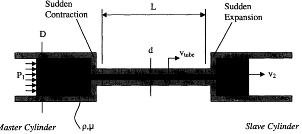
To determine the relative importance of the sources of loss in a hydraulic transmission, a simple hydrostatic system is devised for study. The system of interest takes the form of two hydraulic cylinders connected as shown in Figure 1. This system is

analogous to manual automobile brakes. When a force is applied to the master cylinder, the pressure is transmitted through the fluid and manifests as an output force from the slave cylinder. Sudden Contraction D L Sudden Expansion

Master Cyliinder x P,lJ Slave Cylinder

Figure 1: Cross-sectional drawing of hydraulic cylinders and tubing

To simplify the theoretical analysis, it is initially assumed that the experimental system can be treated as an incompressible steady-flow system. Furthermore, it is

assumed that the flow is laminar and fully-developed. Therefore, the energy equation for incompressible steady-flow stated below can be used to determine the important system characteristics.

+zg

=

+

a

2v2 + zg) ₂+(hfrition +Ehm)g, (1)

where P is the pressure of the fluid, p is the density, a is the kinetic-energy correction factor, v is the velocity, z is the height, g is the acceleration due to gravity, hfrition is the head loss due to friction, and hm is the minor head loss. The subscripts following the parenthetical expressions denote the positions in the fluid flow where the parameters are measured.

If the diameters of both pistons are the same and it is assumed that there is no leakage around the piston head seals, mass conservation dictates that vl=v2. Furthermore,

variations in the vertical height of the fluids contribute very little to the energy equation. Explicitly, ZlZ2. Therefore, the above equation reduces to

(2)

P = P2 +(hfr,,jon +h,)g.

P P

Solving Equation (2) for P2 yields

+av2

2.2 Frictional Losses in Fluid Flow

For a viscous fluid flowing through a conduit, some head loss results from the frictional interaction between the fluid and the conduit walls. Initially, it is assumed that the flow regime within the hydraulic tubing is always laminar. For a circular pipe, the laminar head loss, hfrition, is given by

2

L

__

friction am d 2g (4)

wherefiam is the laminar friction factor, L is the length of the hydraulic tubing, d is the diameter of the hydraulic tubing, and Vtube is the fluid velocity in the hydraulic tubing.

The fluid velocity in the hydraulic tubing, Vtube, can be calculated using the mass conservation equation. Since the fluid is modeled as incompressible, the velocity is simply

K D2

Vtube = 4 Vd2 (5)

The laminar friction factor is given in terms of the Reynolds number, Red, as

64 64,u

im = , (6)

Re- d pVtubed'

where ,u is the fluid viscosity. Substituting Equations (5) and (6) in Equation (4) yields the final expression for the frictional head loss,

64U L VtuOe 3 2 Vtue (7)

hfriction 2 (7)

PV tubedd

2g

Note that the frictional losses from the interaction between the fluid and the inside of the cylinders have been neglected. It can be assumed that the fluid velocity and surface area inside the cylinders are small enough such that these contributions can be neglected.

2.3 Minor Losses in Fluid Flow

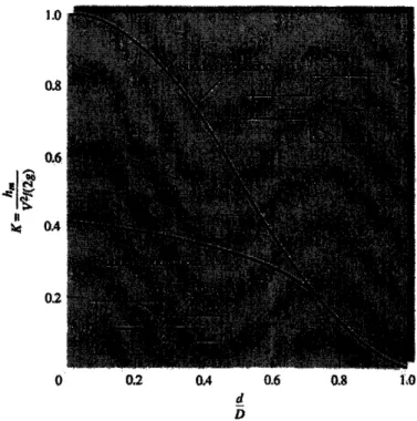
The sudden contractions and expansions in the system due to the working fluid rapidly entering and exiting the cylinders introduce minor losses in the system. Minor losses are typically characterized by the loss coefficient, K. Multiplying the loss coefficient by the velocity head of the fluid, v2/2g, yields the head loss through the

device, hm.

(8)

hm = K Vtube

2g

Figure 2 shows the approximate K factor values as the ratio between the diameters of the small and large conduit sections vary.

1.0 08 1 0.6 OA 02 0 0.2 0.4 0.6 0.8 1iO d D

Figure 2: K factors due to sudden expansions and contractions [2]

Substituting Equations (7) and (8) into Equation (3) yields

= 32uLVtbe ' EK 2

Pg

P2=pipgd 2 + .. g Ip d2 g 2 (9)

The second component on the right-hand side of Equation (9) represents the pressure loss due to friction between the working fluid and the walls of the hydraulic tubing. The third component represents the pressure losses due to the minor losses in the system.

2.4 Seal Friction

Typical working figures for frictional losses in hydraulic cylinders generally vary from 2% to 5% [3]. The exact quantification of forces introduced by seal friction poses a difficult problem. These forces are dependent on seal design, material, fluid and fluid pressure, temperature, rubbing speed, surface finish, and several additional factors [4]. Furthermore, cylinder manufacturers rarely specify frictional loss information. An initial estimate for seal friction is taken from the Seals and Sealing Handbook. Assuming that the cylinders are manufactured with two o-ring seals (one installed on the piston head and another on the rod side), the friction can be approximated by the following equation:

Ffrition = (f xL)+(fh XA) , (10)

where Ffri,tion is the total force due to seal friction,f, is the friction due to o-ring compression, L is the length of the seal rubbing surface, fh is the friction due to fluid pressure, and A is the projected area of seal. Tables and charts given in the Seals and

Sealing Handbook give approximations for these parameters. Assuming the piston o-ring has a 1" OD, the rod o-ring has a 5/16" OD, both o-rings are under a moderate

compression of 15%, both o-rings have a hardness of 70, and the working fluid pressure is -100 psi, the parameters have values given in Table 1.

Table 1

O-ring OD fc L fh A

(in) (lbs-force/in) (in) (lbs-force/in 2) (in2)

1 1 3.14 12 0.17

5/16 1 0.58 12 0.05

Therefore, the total value of Ffriction for both cylinders is 12.72 lbs-force (103.6 N). This is a very high estimate for the frictional forces induced by the internal seals as it is clear from simply actuating the cylinders by hand that the true frictional forces are

considerably lower.

The final equation for the output pressure of the system given the input pressure is

P2 32/ V tu E K PVtube friction

P2 =P1 d2 tb2 D2 (11)

3.0 Experimental Procedure

The importance of Equation (11) is highlighted in Figure 3. The pressure drops due to the loss sources have been translated into force losses by multiplying them by the cylinder bore. For the purposes of illustration, water has been selected as the working fluid, and the hydraulic tubing has a diameter of 1/4" and a length of 16". The cylinder bore is assumed to be 1". It is clear from the figure that both frictional and minor losses

are very small at low flow velocities. Therefore, it is probable that the major source of loss in the system is seal friction.

Figure 3: Force loss sources vs. fluid velocity in hydraulic tubing.

As discussed in Section 2.4, the magnitude of seal friction is dependent upon a number of factors. Seal friction can vary greatly depending on rubbing speed. Since an accurate quantification of seal friction can only be developed empirically, the

experimental analysis will focus on the losses in the system at typical rubbing speeds (-50 cycles per minute) [4].

In order to assess the feasibility of a hydrostatic bicycle transmission, a bench-level experiment was designed and manufactured to measure the efficiency of a simplified hydrostatic transmission. A DC motor with known torque-speed

characteristics was used to cyclically actuate a master cylinder through a linkage system. This master cylinder was connected to a slave cylinder with hydraulic tubing. Constant force springs were used to induce a constant load on the slave cylinder. By operating the motor at a voltage for which the torque-speed characteristics were known, the torque input into the system was deduced from measurement of the angular velocity of the motor shaft.

3.1 Apparatus

The experimental apparatus shown in Figure 4 consists of two double-acting pneumatic cylinders arranged such that they share a common axis. The cylinders have a maximum stroke of 1" (0.0254 m) and a bore diameter of 1" (0.0254 m). A DC motor was used to actuate the master cylinder on the right. The force was transmitted through

the working fluid in the hydraulic tubing to the slave cylinder on the left. Constant force springs were used to apply a constant load to the slave cylinder.

Unfortunately, the manufacturer of the cylinders used for the experiment, ARCO, has been acquired by another corporation and has discontinued the Duramite line.

Consequently, the technical specifications of the cylinders are unattainable. While the exact internal construction is unknown, cylinders of this type typically use Buna-N as the seal material. Double-acting cylinders typically use seals seated in grooves machined around the piston head as well as fixed seals on the piston-rod end. The number of seals in a given type of cylinder can vary depending on the manufacturer, but for the purposes of this analysis, it is assumed that a single seal is used on the piston-rod side, and another

single seal is installed on the piston-head.

Constant Force Power Supply

Springs Master Cylinder

Slave Cylinder

\

f Motor

Figure 4: Experimental apparatus

The cylinders were oriented so that their piston rods pointed in opposite directions as shown in Figure 5. A connection was made between one port from each cylinder with copper tubing. The tubing has a nominal OD of 0.25" and an ID of 0.186". Since the distance from the bottom bracket to the rear-cassette of most bicycles is usually between 16" and 18", the hydraulic tube was cut to a length of 16". The cylinders procured for experimentation are designed for use with air as the working fluid. Since air is highly compressible, it is unsuitable for the purposes of the experiment. For this reason, water, a nearly incompressible fluid, will be used as the hydraulic fluid. The exact operational

specifications of the cylinders are unknown; therefore, for purposes of safety, the fluid pressure inside the cylinders will be kept below a reasonable limit. The rod-side of each cylinder was vented to the atmosphere through the remaining ports.

O Air Open Ports * Water

Piston Rod Piston Head Hydraulic Tubing Cylinder Body

Figure 5: Schematic of experimental cylinder arrangement

Standard hydraulic pipe fittings were used to attach the pipe to the cylinders. In order to ensure that no air bubbles remained in the hydraulic system, one cylinder was first connected to the pipe then completely submerged in a large tank of water. The cylinder was then manually actuated several times to expel any air from the pipe and cylinder. Next, the second cylinder was submerged in the tank and actuated to remove all air. Finally, the cylinders were adjusted such that their strokes were 180° _{out of phase}

before the second cylinder was connected to the pipe. The cylinders were then rigidly secured to mounting plates with their screwed nose connections.

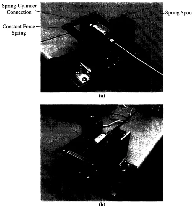
Constant force springs were selected to produce the load on the slave cylinder. Not only do these springs apply a nearly constant force over their extension, they also minimize any inertial loading effects that might arise when using other loading methods e.g. a mass-pulley system. The springs used produce a load of 10.6 lbs-force (47.2 N) each. A total of four springs were used in the experiment. In accordance with the manufacturer's optimal mounting specifications, each spring was installed on its own Delrin spool. These spools were free to rotate as the springs extended and contracted nearly eliminating all frictional resistance. Additionally, the springs were mounted back to back increasing the stability of the exerted force. Figure 6 illustrates how the springs were mounted and attached to the slave piston-rod. The spring-cylinder connection was designed such that the spring force would be delivered to the piston-rod along the approximate axis of the cylinder. This was done to help minimize side loading on the slave piston-rod and the resulting frictional losses.

---- Li I I

Spring-Cylinder Connection Constant Force -Spring -Spring Spool (a) (b)

Figure 6: Spring-cylinder module. (a) Note that only two springs are

attached to the cylinder in this photograph. (b) Note that the spring force is directed along the cylinder axis.

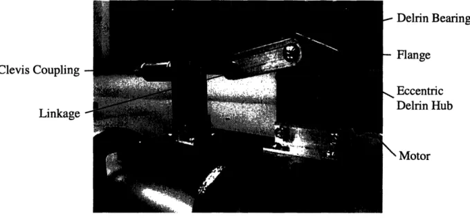
The DC motor used to actuate the master cylinder was manufactured by the Ford Motor Company. It was originally designed to power the windshield wipers on

automobiles. The motor is capable of producing reasonably high torque at low speed which makes it suitable for simulating the energy input from a human rider. The motor can be operated in several modes depending on how it is connected. The torque-speed curves for the various modes have been determined experimentally at a nominal voltage of 13.8 V [5]. A linkage system was designed to convert rotational motion into

joint. The motor was powered using a Model #1760A BK Precision Triple Output DC Power Supply at a constant voltage of 13.8V. Figure 7 illustrates the motor module.

Clevis Coupling Linkage -- Delrin Bearing - Flange Eccentric Delrin Hub

\ Motor

Figure 7: Motor module

The torque-speed curves for the two operational modes used during experimentation are shown in Figure 8. The equation of the line in Figure 8a is

=--0.0926w+7.5, and the equation for the right-most line segment in Figure 8b is

z=-0.5w+25.

Torque-Speed for Ford Motor, Yellow & White wires,

CW direction (1S-L2S \ 8 7 a E 5

z

4

(b)

Figure 8: Torque-speed curves for the Ford motor. (a) High speed mode

(yellow and white connections). (b) High torque mode (black and white connections).

3.2 Methods

Three experiments were conducted with the test apparatus. First, the slave cylinder was disconnected from the constant force springs and the motor was powered in high-speed mode. The motor was wired to spin the shaft in the clockwise direction when viewed from the shaft side. The power supply was adjusted to produce a constant 13.8V,

and the system was allowed to reach steady state operation (the motor has a time constant of approximately 2 seconds). Next, a Panasonic DVX100 video camera was used to film the linkage system attached to the motor during operation. By analyzing the film frame by frame, the rotational angle of the motor shaft can be determined. The camera records 24 frames per second, so two consecutive frames are separated by -0.04167 seconds. Angle and time data was logged for five full revolutions of the motor shaft.

Next, two constant force springs were connected to the slave cylinder. The motor was then powered in high-torque mode by using the white and black connections. The power supply was adjusted to produce a constant voltage of 13.8 V. The motor was

allowed to reach full speed before the data was recorded with the video camera.

Finally, all four constant force springs were connected to the slave cylinder. The motor connections and power supply output were maintained from the previous

experiment, and data was logged using the video camera.

The angular position of the motor shaft was plotted against time. Additionally, the time-varying angular velocity of the motor shaft was calculated by taking the difference between each consecutive angle measurement and dividing by the time duration between each frame of the video. By using the torque-speed curves of the motor, the time-varying output torque was determined.

Torque-Speed for Ford Motor, Black & White wires,

CW direction I t 12 10 4 2 0 0 10 20 30 40 50 Speed (RPM 1

4.0 Results

Shown below in Figure 9 are the results for the test conducted with two constant force springs with the motor wired for high-torque operation. The angular position of the motor shaft as a function of time is very nearly a linear function.

Angular Position vs. Time

U5 E 10 -.2 15 -o -20 -a. _a 25 C 30 -' 35 40 -0 2 4 6 8 Time (s)

..':_ -

'i..._

.'

:

_{... _,...}

_..

_{. ...}

Figure 9: Graph of angular position vs. time for the two springs, high-torque test.

Figure 10 below shows the angular velocity of the motor shaft as a function of time.

Angular Velocity vs. Time

* *** **** * -** . * . ... ** . .. .. *6 ... *v * _. __l* 2 -.. _HLl w...L. .WW .W 10 # -* * * ** 4 Time (s) 6

Figure 10: Graph of angular velocity vs. time for the two springs, high-torque test.

co 3 0) -3 -3.5 -4 -4.5 -5 -5.5 -6 0 8

- --LC ---

I--- ---

__ILYI·-- --- I---I-

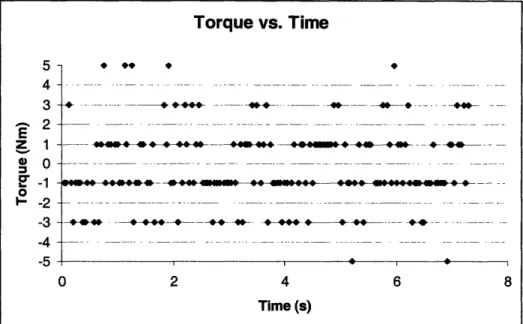
Figure 11 shows the variation of the motor's output torque with time. This data was generated by using experimental velocities and the torque speed curves shown in Figure

8. ;, 4 3 - 2 E

z 1

_o

-Figure 11: Graph of torque vs. time for the two springs, high-torque test.

The no-load test was conducted mainly for safety considerations. The data collected from this experiment can be seen in Appendix A. Data for the test conducted with four springs was not collected. The power supply was incapable of operating the motor with the large load without constantly varying the input voltage. Since the

torque-speed characteristics of the motor are only known for a nominal input voltage of 13.8 V, the data from this experiment was not valuable for the present analysis.

5.0 Discussion

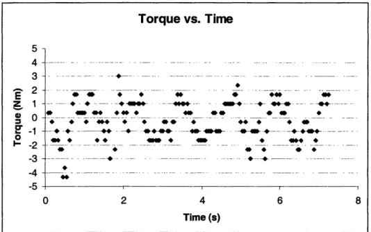
At first glance, the experimental results look somewhat ambiguous; however, taking a three-point average of the torque data points reveals a sinusoidal curve. Figure 12 highlights the sinusoidal characteristics of the torque vs. time plot.

Torque vs. Time .. . .. ... ... _ _ ...-..- ... .*. . . .__. _.... .__... .. . . .__... .. .. _.... _...._. ... .-... . __ q- --- -... ---- .. . _-- ,_ . -... A___ ~ ~ ~ ~ - ~ .___. ' ~~~.. -.; _.., * *_ ~ - -. -

-_

---

-_.

Torque vs. Time 4- 3-- 2 E z 1-0 0--2 --3 4 5 -0 2 4 6 8 Time (s) .. .. ... ... ...s ...- --... -. ....- ... .... . . -- .- . .. -.... . -. .- . . . . ---.. , ... ...- e .---- --- .- ---- 4- --- - -- . ....- . -

-~~~~40~

Figure 12: Graph of torque vs. time for the two springs, high-torque test.

By averaging the values of each three consecutive data points, the sinusoidal behavior of the system becomes clearer.

The transmission efficiency, rM, for bicycles is defined as the energy output at the coupling to the driving wheel divided by the energy delivered by the human body [1].

W

qM = Wt x100, (12)

Win

where Wout is the energy output at the driving wheel, and Wn is the work input from the human rider.

The overall efficiency of the testing apparatus can be determined by applying Equation (12) to the system. Wou, is simply the work done by the cylinder to extend the constant force spring. The extension of the spring was measured during the experiment to be Ax=0.9" (0.0229m). Since the two constant force springs produce a total force of 94.4 N, Wout is

Wout = Fspring x Ax = 94.4N x 0.0229m = 2.16J . (13)

The work input from the motor is analogous to the human rider work input from Equation (12). The motor only does work during one half of the cycle. For the

following half-cycle, the springs exert a restoring force on the cylinder to help return the master cylinder piston-rod to it original orientation. By finding the average torque produced during the first half-cycle, an approximate value for Win can be determined. By multiplying the average torque by the angle through which it acts ( rad), an

approximation of the input work is obtained. I

Win =verage X,_{in average} (14) where ,,,,,average is the average torque delivered by the motor shaft. Table 2 shows the input and output work and the efficiency of the test system. Each row in Table 2 corresponds to the half-cycle when the springs are being extended.

Table 2

Average Torque Work In Work Out Efficiency

(Nm)

(J)

(J)

(%)

Taking the average of the efficiencies calculated in Table 2 yields 69.5%. In order to compare this data to the theoretical model developed in Section 2, Equation (11) must be modified to incorporate the physical load and motor. P2 in Equation (11) is

simply the force applied by the constant force springs divided by the area of the piston head:

Frin

P2 spring (15)

( 4 )

The input pressure, Pi, can be expressed in terms of the motor torque as

p r -rsin

(16)

where r is the motor torque, r is the radial offset of the connecting linkage from the motor shaft, and 0 is the rotation of the motor shaft (positive x-axis taken as zero, positive in the counterclockwise direction). After substituting Equations (15) and (16) into Equation (11) and solving for r, the theoretical motor torque can be plotted as a function of time. The resulting equation was solved using Matlab. The m.file used to generate the plots below can be seen in Appendix B.

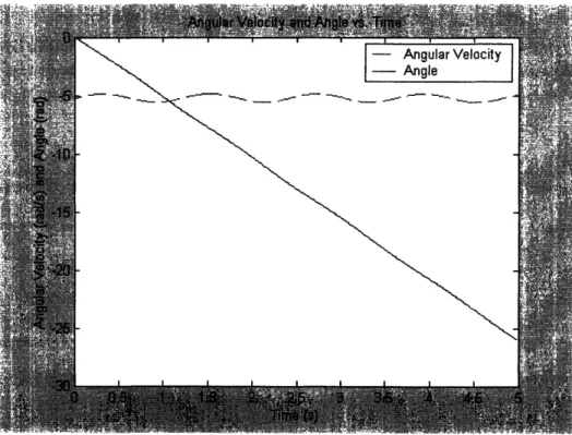
Figure 13 shows the theoretical angular position and velocity of the motor shaft vs. time. Figure 14 show the agreement between the experimental and the theoretical motor torque. There seems to be a reasonably good agreement between the two sets of data, but neither can be fully trusted for reasons outlined in the next section.

Figure 13: Theoretical motor shaft angular position and velocity vs. time.

Figure 14: Theoretical vs. experimental motor torque. Note that the

5.1 Error Analysis

The error in the experimental measurements can be explained by a combination of four factors. First, the power supply used to power the motor had a maximum rated current capacity of 2 A. During the two springs, high-torque experiment, there was a brief moment when the power supply switched to constant current mode. During this time, the voltage was time varying. This would introduce error in the torque calculation

since the known torque-speed curves would no longer be accurate. However, the power supply only switched into constant current mode for a fraction of a second during each cycle, and the voltage only varied -0.2 V during this period. Therefore, most of the error is due to other sources.

The second source of error is the questionable torque-speed data for the motors. The data points on the charts are sparse, and the best fit lines do not detail the associated error. It might be useful to reconstruct these curves in an additional experiment.

The third source of error is associated with the method of determining the angular position of the motor shaft. Figure 15 shows a typical frame used to log data points.

Figure 15: Example frame from experimental recording

Data points were recorded by attaching a transparency of a 360° protractor to the

computer screen. The video was analyzed frame by frame to determine the orientation of the shaft as a function of time. The black dot placed on the bottom corner of the flange in the above photograph was used to compile the data. Each frame taken by the video camera is 1/48 second in duration. Consequently, some blur is introduced in the

individual images. Due to the methods used to log the data, there is an associated error of +1°in all data points. This translates to an error of +4 Nm in the experimental torque. 5.2 Experimental Design Flaws

Unfortunately, the results of the experiment are of limited to no value. Oversights in the design of the experimental apparatus led to additional losses in the system that could not be measured nor separated from the losses of interest. Namely, no precautions were made to prevent side-loading on the piston-rods. This means that large frictional

forces could have developed inside the cylinders. This would make the observed losses far more substantial than if proper measures had been taken to ensure that only axial loads were transmitted. Since the side-loading of the piston-rods could not be directly measured, it was not possible to separate the resulting losses from the seal friction losses of interest.

Another shortcoming of the experiment was the use of water instead of oil as the working fluid. Water was initially selected for its convenience and availability (see Section 3.1); however, it is probable that the frictional losses in the system could have been considerably lower if oil had been used in place of water.

The primary downfall of the documented experiment is due to its complexity. The experiment was designed to measure the losses in the hydrostatic transmission during cyclical actuation. The way that the actuation was implemented introduced

immeasurable losses due to side-loading of the cylinders that were outside the scope of the analysis. A more reasonable approach to this design problem would have been to investigate one aspect of the system at a time. A suitable initial experiment would have been a simple analysis of the system shown in Figure 1. If the input and output forces of the system could be accurately measured during low speed actuation, the efficiency of the cylinder system alone could be isolated. If the losses in this simple system were

sufficiently low, experimentation could continue to determine the losses during low speed cyclical actuation with the proper precautions taken to limit side-loading of the piston rods.

6.0 Prototype Design

Designing a functional prototype of a hydrostatic bicycle transmission is considerably more difficult than designing a simple testing apparatus. There are many considerations that must be taken that were not as important during experimentation. The difficulty is compounded by the fact that most hydraulic machinery is designed for industrial use. Typically, nominal operating speeds and pressures of OEM components are considerably higher than those necessary for a human power application.

Furthermore, most models are prohibitively massive and bulky for installation on a bicycle. For example, an entry in Parker Hannifin's "Chainless Challenge," a new competition challenging university students to develop a hydraulic or pneumatic

alternative for the standard chain-based bicycle transmission, weighed a hefty 137 pounds. The hydraulic system alone accounted for approximately 61 pounds [6]. The following design suggestions are intended to reduce weight and complexity of the system while generating high efficiencies.

6.1 Pump and Motor Design

The hydraulic pump is one of the two primary components of the hydrostatic drive. Perhaps the most useful information gathered from the experiment is the necessity of using some mechanism to minimize side-loading on the pistons. The pump selected for this application is a horizontal, triplex, piston, power-pump. This type of pump can be easily fitted with crossheads to virtually eliminate side-loading. Its construction is very similar to that of an internal combustion engine. Three eccentrics are mounted on a straight shaft with a 120° _{phase shift between each. The eccentricity of the cams is}

exactly half the length of the desired piston stroke. Connecting rods mounted on low-friction sleeve bearings connect the crankshaft to the crossheads at the wrist pin. The

crossheads are in turn connected to the piston rods and are free to slide in linear motion within the crossways.

There are several factors that lead to this design choice. These pumps are generally characterized by high mechanical efficiencies. Overall efficiencies typically range from 85% to 95% [7]. Other pump choices offer useful features but cannot

produce competitive efficiencies. The axial piston pump with adjustable swash plate, for instance, can be used as part of a continuously variable transmission. However, the operating efficiencies are far too low to be competitive with chains and rear cassettes. Second, other design choices are simply too bulky for the bicycle application.

A three-piston design was selected to eliminate the possibility of a top-dead-center condition. Additionally, using multiple cylinders will help remedy the problem of pulsing flow generally associated with reciprocating pumps.

This type of device could be used as the hydraulic motor as well, by simply operating the system in reverse.

6.2 Hydraulic Tubing and Fluid Selection

An important consideration in the design of the hydrostatic transmission is the selection of the hydraulic tubing. The tubing must obviously withstand significant

internal pressures without rupturing, but it must also resist elastic deformation as much as possible. If a highly elastic material was used as the hydraulic tubing, it would undergo deformation during use. The strain energy associated with the deformation would reduce the overall efficiency of the system. Furthermore, deformation of the hydraulic tubing would reduce the effective stroke of the slave cylinder. For these reasons, it is important to select a sufficiently inelastic material for the hydraulic tubing. For a thin-walled cylindrical pressure-vessel, the hoop stress is given by

P r , (17)

t

where a is the hoop stress, Pin, is the internal pressure, r is the radius of the pressure vessel, and t it the wall thickness. Strain energy per unit volume can then be calculated as

2

u = , (18)

2E

where u is the strain energy per unit volume, and E is the modulus of elasticity. From Equation (18) it is clear that a higher modulus of elasticity will decrease the strain energy. Finally, the strain energy in the hydraulic pipe is approximated by

U = 8 zd3 _{L, (19)}

For the purposes of the prototype, steel piping of 1/4" OD and 0.049" wall thickness can be used. In future designs, it may be beneficial to find a lower weight solution. The total strain energy in a 16" pipe at a very high operating pressure estimate of 2500 psi is a minute 0.046 J.

As mentioned in Section 5.2, hydraulic oil should be used as the working fluid instead of water. This will help reduce frictional losses due to fluid viscosity.

Additionally, an accumulator should be connected to each hydraulic line to accommodate for any losses of the hydraulic fluid at the seal interfaces.

6.3 Cylinder Selection

Cylinder selection is the most important factor in the design of the hydraulic bicycle. The majority of the losses in the system can be expected to stem from the seals within the cylinders; therefore, it will be beneficial to select cylinders with minimal frictional losses at typical operating speeds and pressures. An empirical study of seal friction losses in potential cylinders should precede their implementation in the prototype.

7.0 Future Work

With additional time and resources, a simplified experiment would be constructed consisting of two cylinders connected as shown in Figure 1. The apparatus would be constructed to directly and accurately measure the input and output forces in the system. Thus, the efficiency of the isolated cylinder-to-cylinder system could be determined. Depending on the results of this experiment, improvements could be made to the current experimental apparatus to limit side loading on the cylinder piston-rods. Additionally, a better method of measuring the input torque from the motor would be implemented, or an entirely new method of cyclical actuation and loading would be devised.

8.0 References

[1] Wilson, David G., Bicycling Science, Third Edition. Cambridge, MA: The MIT Press, 2004.

[2] White, Frank M., Fluid Mechanics, Fourth Edition. Boston, MA: McGraw-Hill Companies, Inc., 1999.

[3] Brunell, R., Hydraulic & Pneumatic Cylinders. Morden, Surrey, England: Trade & Technical Press Ltd.

[4] Warring, R.H., Seals and Sealing Handbook, First Edition. Houston, TX: Gulf Publishing Co., 1981.

[5] "Ford Windshield Wiper Motor." 2.007 Webpage, January 1, 2006 <http://pergatory.mit.edu/2.007/kit/actuator/fordmtr/fordmtr.html> [6] "Unchained Innovation." MachineDesign.com, January 12, 2006

<http://www.machinedesign.com/ASP/viewSelectedArticle.asp?strArticleId=59280&strS ite=MDSite&catId=0>

[7] Henshaw, Terry L., Reciprocating Pumps. New York, NY: Van Nostrand Reinhold Co., 1987.

Appendix A

The following data was collected for the no-load, high-speed experiment.

Time (s) 0.000 0.042 0.083 0.125 0.167 0.208 0.250 0.292 0.333 0.375 0.417 0.458 0.500 0.542 0.583 0.625 0.667 0.708 0.750 0.792 0.833 0.875 0.917 0.958 1.000 1.042 1.083 1.125 1.167 1.208 1.250 1.292 1.333 1.375 1.417 1.458 1.500 1.542 1.583 Angle (deg) 0 340 319 299 278 259 238 217 197 176 156 136 115 96 74 54 34 13 353 332 312 292 271 250 230 210 190 169 149 128 108 88 67 47 26 6 346 325 305 Normalized Absolute Angle (deg) 0 -20 -41 -61 -82 -101 -122 -143 -163 -184 -204 -224 -245 -264 -286 -306 -326 -347 -367 -388 -408 -428 -449 -470 -490 -510 -530 -551 -571 -592 -612 -632 -653 -673 -694 -714 -734 -755 -775 Table Al Time (s) 1.708 1.750 1.792 1.833 1.875 1.917 1.958 2.000 2.042 2.083 2.125 2.167 2.208 2.250 2.292 2.333 2.375 2.417 2.458 2.500 2.542 2.583 2.625 2.667 2.708 2.750 2.792 2.833 2.875 2.917 2.958 3.000 3.042 3.083 3.125 3.167 3.208 3.250 3.292 Angle (deg) 244 224 203 182 162 142 121 101 80 61 40 19 359 338 318 298 277 257 236 217 196 175 155 134 114 94 73 53 32 12 352 331 311 290 270 250 229 209 188 Normalized Absolute Angle (deg) -836 -856 -877 -898 -918 -938 -959 -979 -1000 -1019 -1040 -1061 -1081 -1102 -1122 -1142 -1163 -1183 -1204 -1223 -1244 -1265 -1285 -1306 -1326 -1346 -1367 -1387 -1408 -1428 -1448 -1469 -1489 -1510 -1530 -1550 -1571 -1591 -1612 Time (s) 3.417 3.458 3.500 3.542 3.583 3.625 3.667 3.708 3.750 3.792 3.833 3.875 3.917 3.958 4.000 4.042 4.083 4.125 4.167 4.208 4.250 4.292 4.333 4.375 4.417 4.458 4.500 4.542 4.583 4.625 4.667 4.708 4.750 4.792 4.833 4.875 4.917 4.958 5.000 Angle (deg) 127 107 86 65 46 25 5 344 324 304 283 263 242 221 202 181 161 140 120 100 79 59 38 18 358 337 317 296 276 256 235 214 194 174 154 133 113 92 71 Normalized Absolute Angle (deg) -1673 -1693 -1714 -1735 -1754 -1775 -1795 -1816 -1836 -1856 -1877 -1897 -1918 -1939 -1958 -1979 -1999 -2020 -2040 -2060 -2081 -2101 -2122 -2142 -2162 -2183 -2203 -2224 -2244 -2264 -2285 -2306 -2326 -2346 -2366 -2387 -2407 -2428 -2449

The following data was collected for the two springs, high-torque experiment. Angle (deg) 358 343 332 320 308 295 282 271 259 247 234 223 214 205 194 180 167 152 140 128 114 103 90 78 64 51 39 25 13 0 346 333 321 309 297 285 274 262 250 238 227 215 203 Normalized Absolute Angle (deg) -2 -17 -28 -40 -52 -65 -78 -89 -101 -113 -126 -137 -146 -155 -166 -180 -193 -208 -220 -232 -246 -257 -270 -282 -296 -309 -321 -335 -347 -360 -374 -387 -399 -411 -423 -435 -446 -458 -470 -482 -493 -505 -517 Angle (rad) -0.035 -0.297 -0.489 -0.698 -0.908 -1.134 -1.361 -1.553 -1.763 -1.972 -2.199 -2.391 -2.548 -2.705 -2.897 -3.142 -3.368 -3.630 -3.840 -4.049 -4.294 -4.485 -4.712 -4.922 -5.166 -5.393 -5.603 -5.847 -6.056 -6.283 -6.528 -6.754 -6.964 -7.173 -7.383 -7.592 -7.784 -7.994 -8.203 -8.412 -8.604 -8.814 -9.023 Table A2 Angular Velocity (rad/s) -6.283 -4.608 -5.027 -5.027 -5.445 -5.445 -4.608 -5.027 -5.027 -5.445 -4.608 -3.770 -3.770 -4.608 -5.864 -5.445 -6.283 -5.027 -5.027 -5.864 -4.608 -5.445 -5.027 -5.864 -5.445 -5.027 -5.864 -5.027 -5.445 -5.864 -5.445 -5.027 -5.027 -5.027 -5.027 -4.608 -5.027 -5.027 -5.027 -4.608 -5.027 -5.027 -5.027 Angular Velocity (RPM) -60 -44 -48 -48 -52 -52 -44 -48 -48 -52 -44 -36 -36 -44 -56 -52 -60 -48 -48 -56 -44 -52 -48 -56 -52 -48 -56 -48 -52 -56 -52 -48 -48 -48 -48 -44 -48 -48 -48 -44 -48 -48 -48 3-Point Average (RPM) -52.000 -50.667 -46.667 -49.333 -50.667 -49.333 -48.000 -46.667 -49.333 -48.000 -44.000 -38.667 -38.667 -45.333 -50.667 -56.000 -53.333 -52.000 -50.667 -49.333 -50.667 -48.000 -52.000 -52.000 -52.000 -52.000 -50.667 -52.000 -52.000 -53.333 -52.000 -49.333 -48.000 -48.000 -46.667 -46.667 -46.667 -48.000 -46.667 -46.667 -46.667 -48.000 -48.000 Torque (Nm) 5 -3 -1 -1 1 1 -3 -1 -1 1 -3 -7 -7 -3 3 1 5 -1 -1 3 -3 1 -1 3 1 -1 3 -1 1 3 1 -1 -1 -1 -1 -3 -1 -1 -1 -3 -1 -1 -1 Time (s) 0.000 0.042 0.083 0.125 0.167 0.208 0.250 0.292 0.333 0.375 0.417 0.458 0.500 0.542 0.583 0.625 0.667 0.708 0.750 0.792 0.833 0.875 0.917 0.958 1.000 1.042 1.083 1.125 1.167 1.208 1.250 1.292 1.333 1.375 1.417 1.458 1.500 1.542 1.583 1.625 1.667 1.708 1.750 3-Point Average Torque (Nm) 1.00 0.33 -1.67 -0.33 0.33 -0.33 -1.00 -1.67 -0.33 -1.00 -3.00 -5.67 -5.67 -2.33 0.33 3.00 1.67 1.00 0.33 -0.33 0.33 -1.00 1.00 1.00 1.00 1.00 0.33 1.00 1.00 1.67 1.00 -0.33 -1.00 -1.00 -1.67 -1.67 -1.67 -1.00 -1.67 -1.67 -1.67 -1.00 -1.00 -..

1.792 1.833 1.875 1.917 1.958 2.000 2.042 2.083 2.125 2.167 2.208 2.250 2.292 2.333 2.375 2.417 2.458 2.500 2.542 2.583 2.625 2.667 2.708 2.750 2.792 2.833 2.875 2.917 2.958 3.000 3.042 3.083 3.125 3.167 3.208 3.250 3.292 3.333 3.375 3.417 3.458 3.500 3.542 3.583 3.625 3.667 3.708 3.750 3.792 3.833 191 179 166 154 143 130 119 106 93 80 66 54 40 27 15 2 348 337 324 312 300 288 276 265 253 241 230 218 205 194 182 169 156 144 133 120 108 95 82 69 56 43 30 17 4 350 337 323 311 300 -529 -541 -554 -566 -577 -590 -601 -614 -627 -640 -654 -666 -680 -693 -705 -718 -732 -743 -756 -768 -780 -792 -804 -815 -827 -839 -850 -862 -875 -886 -898 -911 -924 -936 -947 -960 -972 -985 -998 -1011 -1024 -1037 -1050 -1063 -1076 -1090 -1103 -1117 -1129 -1140 -9.233 -9.442 -9.669 -9.879 -10.071 -10.297 -10.489 -10.716 -10.943 -11.170 -11.414 -11.624 -11.868 -12.095 -12.305 -12.531 -12.776 -12.968 -13.195 -13.404 -13.614 -13.823 -14.032 -14.224 -14.434 -14.643 -14.835 -15.045 -15.272 -15.464 -15.673 -15.900 -16.127 -16.336 -16.528 -16.755 -16.965 -17.191 -17.418 -17.645 -17.872 -18.099 -18.326 -18.553 -18.780 -19.024 -19.251 -19.495 -19.705 -19.897 -5.027 -5.445 -5.027 -4.608 -5.445 -4.608 -5.445 -5.445 -5.445 -5.864 -5.027 -5.864 -5.445 -5.027 -5.445 -5.864 -4.608 -5.445 -5.027 -5.027 -5.027 -5.027 -4.608 -5.027 -5.027 -4.608 -5.027 -5.445 -4.608 -5.027 -5.445 -5.445 -5.027 -4.608 -5.445 -5.027 -5.445 -5.445 -5.445 -5.445 -5.445 -5.445 -5.445 -5.445 -5.864 -5.445 -5.864 -5.027 -4.608 -5.445 -48 -52 -48 -44 -52 -44 -52 -52 -52 -56 -48 -56 -52 -48 -52 -56 -44 -52 -48 -48 -48 -48 -44 -48 -48 -44 -48 -52 -44 -48 -52 -52 -48 -44 -52 -48 -52 -52 -52 -52 -52 -52 -52 -52 -56 -52 -56 -48 -44 -52 -49.333 -49.333 -48.000 -48.000 -46.667 -49.333 -49.333 -52.000 -53.333 -52.000 -53.333 -52.000 -52.000 -50.667 -52.000 -50.667 -50.667 -48.000 -49.333 -48.000 -48.000 -46.667 -46.667 -46.667 -46.667 -46.667 -48.000 -48.000 -48.000 -48.000 -50.667 -50.667 -48.000 -48.000 -48.000 -50.667 -50.667 -52.000 -52.000 -52.000 -52.000 -52.000 -52.000 -53.333 -53.333 -54.667 -52.000 -49.333 -48.000 -48.000 -1 1 -1 -3 1 -3 1 1 1 3 -1 3 1 -1 1 3 -3 1 -1 -1 -1 -1 -3 -1 -1 -3 -1 1 -3 -1 1 1 -1 -3 1 -1 1 1 1 1 1 1 1 1 3 1 3 -1 -3 -0.33 -0.33 -1.00 -1.00 -1.67 -0.33 -0.33 1.00 1.67 1.00 1.67 1.00 1.00 0.33 1.00 0.33 0.33 -1.00 -0.33 -1.00 -1.00 -1.67 -1.67 -1.67 -1.67 -1.67 -1.00 -1.00 -1.00 -1.00 0.33 0.33 -1.00 -1.00 -1.00 0.33 0.33 1.00 1.00 1.00 1.00 1.00 1.00 1.67 1.67 2.33 1.00 -0.33 -1.00 -1.00 -. ,. - -. ... . . .

3.875 3.917 3.958 4.000 4.042 4.083 4.125 4.167 4.208 4.250 4.292 4.333 4.375 4.417 4.458 4.500 4.542 4.583 4.625 4.667 4.708 4.750 4.792 4.833 4.875 4.917 4.958 5.000 5.042 5.083 5.125 5.167 5.208 5.250 5.292 5.333 5.375 5.417 5.458 5.500 5.542 5.583 5.625 5.667 5.708 5.750 5.792 5.833 5.875 5.917 287 275 263 253 241 230 217 205 194 181 168 155 146 134 122 110 96 84 70 57 45 30 18 5 352 340 327 313 301 290 278 266 254 243 232 220 208 196 183 171 159 147 135 123 113 100 87 75 61 48 -1153 -1165 -1177 -1187 -1199 -1210 -1223 -1235 -1246 -1259 -1272 -1285 -1294 -1306 -1318 -1330 -1344 -1356 -1370 -1383 -1395 -1410 -1422 -1435 -1448 -1460 -1473 -1487 -1499 -1510 -1522 -1534 -1546 -1557 -1568 -1580 -1592 -1604 -1617 -1629 -1641 -1653 -1665 -1677 -1687 -1700 -1713 -1725 -1739 -1752 -20.124 -20.333 -20.543 -20.717 -20.926 -21.118 -21.345 -21.555 -21.747 -21.974 -22.201 -22.427 -22.585 -22.794 -23.003 -23.213 -23.457 -23.667 -23.911 -24.138 -24.347 -24.609 -24.819 -25.045 -25.272 -25.482 -25.709 -25.953 -26.162 -26.354 -26.564 -26.773 -26.983 -27.175 -27.367 -27.576 -27.786 -27.995 -28.222 -28.431 -28.641 -28.850 -29.060 -29.269 -29.444 -29.671 -29.897 -30.107 -30.351 -30.578 -5.027 -5.027 -4.189 -5.027 -4.608 -5.445 -5.027 -4.608 -5.445 -5.445 -5.445 -3.770 -5.027 -5.027 -5.027 -5.864 -5.027 -5.864 -5.445 -5.027 -6.283 -5.027 -5.445 -5.445 -5.027 -5.445 -5.864 -5.027 -4.608 -5.027 -5.027 -5.027 -4.608 -4.608 -5.027 -5.027 -5.027 -5.445 -5.027 -5.027 -5.027 -5.027 -5.027 -4.189 -5.445 -5.445 -5.027 -5.864 -5.445 -5.445 -48 -48 -40 -48 -44 -52 -48 -44 -52 -52 -52 -36 -48 -48 -48 -56 -48 -56 -52 -48 -60 -48 -52 -52 -48 -52 -56 -48 -44 -48 -48 -48 -44 -44 -48 -48 -48 -52 -48 -48 -48 -48 -48 -40 -52 -52 -48 -56 -52 -52 -49.333 -45.333 -45.333 -44.000 -48.000 -48.000 -48.000 -48.000 -49.333 -52.000 -46.667 -45.333 -44.000 -48.000 -50.667 -50.667 -53.333 -52.000 -52.000 -53.333 -52.000 -53.333 -50.667 -50.667 -50.667 -52.000 -52.000 -49.333 -46.667 -46.667 -48.000 -46.667 -45.333 -45.333 -46.667 -48.000 -49.333 -49.333 -49.333 -48.000 -48.000 -48.000 -45.333 -46.667 -48.000 -50.667 -52.000 -52.000 -53.333 -53.333 -0.33 -2.33 -2.33 -3.00 -1.00 -1.00 -1.00 -1.00 -0.33 1.00 -1.67 -2.33 -3.00 -1.00 0.33 0.33 1.67 1.00 1.00 1.67 1.00 1.67 0.33 0.33 0.33 1.00 1.00 -0.33 -1.67 -1.67 -1.00 -1.67 -2.33 -2.33 -1.67 -1.00 -0.33 -0.33 -0.33 -1.00 -1.00 -1.00 -2.33 -1.67 -1.00 0.33 1.00 1.00 1.67 1.67 -1 -1 -5 -1 -3 1 -1 -3 1 1 1 -7 -1 -1 -1 3 -1 3 1 -1 5 -1 1 1 -1 1 3 -1 -3 -1 -1 -1 -3 -3 -1 -1 -1 1 -1 -1 -1 -1 -1 -5 1 1 -1 3 1 1 |

5.958 35 -1765 -30.805 -5.864 -56 -52.000 3 1.00

6.000 21 -1779 -31.049 -5.027 -48 -53.333 -1 1.67

6.042 9 -1791 -31.259 -5.864 -56 -52.000 3 1.00

Appendix B

The following Matlab m.file was used to find the theoretical efficiency of the testing apparatus. %Motor r=(.45*0.0254); %m %Hydraulic Fluid rho=1000; %kg/m^3 mu=0.001; %kg/m*s %Cylinder D=0.0254; %m %Tubing d=0.0254*.2; %m L=16*.0254; %m %Loss Factors Ffriction=56.6; %N Kcontraction=0.4; Kexpansion=0.9; Ktotal=Kexpansion+Kcontraction; %Springs / Input SpringForce_lbs=10.6; %lbs SpringForce_N=SpringForce_lbs*4.448221; %N SpringCount=2; F2=-SpringForce_N*SpringCount; %N P2=(F2*4)/(pi*DA2); %N/m^2 %Environment g=9.8; %m/s^2 theta=0; %rad w=O; %rad/s t=O; %s

t_duration=5; MotorStats=[]; FluidStats=[]; while length(t)<((t_duration/t_increment)+tincrement) theta=[theta theta(length(theta))+w(length(w))*tincrement]; vl=w(length(w)).*r.*sin(theta(length(theta))); vtube=(D^_2/dA2)*vl; P1=P2-(32*mu*L*vtube/dA2)-(Ktotal*rho*abs(vtube)*vtube/2); F1=(P1 *(pi*D2)/4)-Ffriction; tau=F1 *r* -sin(theta(length(theta))); w=[w (tau+25)/-4.775]; t=[t t(length(t))+t_increment];

MotorStats=[MotorStats; tau F1 w(:,(length(w)- 1))*60/(2*pi)]; FluidStats=[FluidStats; P1 P2 vtube]; end figure(l) clf plot(t,w,'r-') hold on plot(t,theta,'b')

title('Angular Velocity and Angle vs. Time') xlabel('Time (s)')

ylabel('Angular Velocity (rad/s) and Angle (rad)') legend('Angular Velocity','Angle')

figure(2) clf hold on

plot(t(1 :length(t)- 1), MotorStats(:,1)) title('Torque vs. Time')

xlabel('Time (s)') ylabel('Torque (Nm)')

Appendix C

This three-dimensional representation of the experimental apparatus was prepared in SolidWorks to ease the manufacturing and integration processes. The CAD model looks almost identical to the physical apparatus.