HAL Id: hal-02927850
https://hal.archives-ouvertes.fr/hal-02927850
Submitted on 8 Sep 2020
HAL is a multi-disciplinary open access
archive for the deposit and dissemination of
sci-entific research documents, whether they are
pub-lished or not. The documents may come from
teaching and research institutions in France or
abroad, or from public or private research centers.
L’archive ouverte pluridisciplinaire HAL, est
destinée au dépôt et à la diffusion de documents
scientifiques de niveau recherche, publiés ou non,
émanant des établissements d’enseignement et de
recherche français ou étrangers, des laboratoires
publics ou privés.
from site to continental scale: uncertainties arising from
model structure and parameter values
A. Valade, P. Ciais, N. Vuichard, N. Viovy, A. Caubel, N. Huth, F. Marin,
J.-F. Martiné
To cite this version:
A. Valade, P. Ciais, N. Vuichard, N. Viovy, A. Caubel, et al.. Modeling sugarcane yield with a
process-based model from site to continental scale: uncertainties arising from model structure and parameter
values. Geoscientific Model Development, European Geosciences Union, 2014, 7 (3), pp.1225-1245.
�10.5194/gmd-7-1225-2014�. �hal-02927850�
www.geosci-model-dev.net/7/1225/2014/ doi:10.5194/gmd-7-1225-2014
© Author(s) 2014. CC Attribution 3.0 License.
Modeling sugarcane yield with a process-based model from site to
continental scale: uncertainties arising from model structure and
parameter values
A. Valade1, P. Ciais1, N. Vuichard1, N. Viovy1, A. Caubel1, N. Huth2, F. Marin3, and J.-F. Martiné4
1LSCE, CEA-CNRS, Gif-sur-Yvette, 91191, France
2CSIRO. Ecosystem Sciences, P.O. Box 102, Toowoomba, Qld, 4350, Australia
3EMBRAPA Informatica Agropecuria, Barão Geraldo, 13083-886 Campinas SP, Brazil
4CIRAD, UR SCA, Saint-Denis, La Réunion, 97408, France
Correspondence to: A. Valade ([email protected])
Received: 30 December 2013 – Published in Geosci. Model Dev. Discuss.: 31 January 2014 Revised: 22 May 2014 – Accepted: 26 May 2014 – Published: 30 June 2014
Abstract. Agro-land surface models (agro-LSM) have been
developed from the integration of specific crop processes into large-scale generic land surface models that allow calculating the spatial distribution and variability of energy, water and carbon fluxes within the soil–vegetation–atmosphere contin-uum. When developing agro-LSM models, particular atten-tion must be given to the effects of crop phenology and man-agement on the turbulent fluxes exchanged with the atmo-sphere, and the underlying water and carbon pools. A part of the uncertainty of agro-LSM models is related to their usu-ally large number of parameters. In this study, we quantify the parameter-values uncertainty in the simulation of sugar-cane biomass production with the agro-LSM ORCHIDEE– STICS, using a multi-regional approach with data from sites in Australia, La Réunion and Brazil. In ORCHIDEE–STICS, two models are chained: STICS, an agronomy model that calculates phenology and management, and ORCHIDEE, a land surface model that calculates biomass and other ecosys-tem variables forced by STICS phenology. First, the param-eters that dominate the uncertainty of simulated biomass at harvest date are determined through a screening of 67 differ-ent parameters of both STICS and ORCHIDEE on a multi-site basis. Secondly, the uncertainty of harvested biomass attributable to those most sensitive parameters is quantified and specifically attributed to either STICS (phenology, man-agement) or to ORCHIDEE (other ecosystem variables in-cluding biomass) through distinct Monte Carlo runs. The un-certainty on parameter values is constrained using observa-tions by calibrating the model independently at seven sites.
In a third step, a sensitivity analysis is carried out by vary-ing the most sensitive parameters to investigate their effects at continental scale. A Monte Carlo sampling method associ-ated with the calculation of partial ranked correlation coeffi-cients is used to quantify the sensitivity of harvested biomass to input parameters on a continental scale across the large regions of intensive sugarcane cultivation in Australia and Brazil. The ten parameters driving most of the uncertainty in the ORCHIDEE–STICS modeled biomass at the 7 sites are identified by the screening procedure. We found that the 10 most sensitive parameters control phenology (maximum rate of increase of LAI) and root uptake of water and nitro-gen (root profile and root growth rate, nitronitro-gen stress thresh-old) in STICS, and photosynthesis (optimal temperature of photosynthesis, optimal carboxylation rate), radiation inter-ception (extinction coefficient), and transpiration and ration (stomatal conductance, growth and maintenance respi-ration coefficients) in ORCHIDEE. We find that the optimal carboxylation rate and photosynthesis temperature parame-ters contribute most to the uncertainty in harvested biomass simulations at site scale. The spatial variation of the ranked correlation between input parameters and modeled biomass at harvest is well explained by rain and temperature drivers, suggesting different climate-mediated sensitivities of mod-eled sugarcane yield to the model parameters, for Australia and Brazil. This study reveals the spatial and temporal pat-terns of uncertainty variability for a highly parameterized agro-LSM and calls for more systematic uncertainty analy-ses of such models.
1 Introduction
In recent years, many governments have set targets in terms of biofuels consumption for transportation fuel (Sorda et al., 2010), resulting in a large increase in bioenergy cropping area around the world. Concerns about energy shortage,
pol-icy to reduce CO2emissions, and the search for new income
for farmers can explain why energy policies have considered biofuels as a serious alternative to fossil fuel in many coun-tries (Demirbas, 2008). Yet, the claimed benefits of biofuels for fossil fuel substitution have been questioned in terms of
their net effect on atmospheric CO2 and climate, and even
of their economic return (Doornbosch and Steenblik, 2008; Naylor et al., 2007). In particular, the conditions of biofuel cultivation, such as the type of crop, practice, previous land use, and local climate, have emerged as key factors that de-termine the effectiveness of their carbon emissions reduction (Fargione et al., 2008; Hill et al., 2006; Searchinger et al., 2008). At the heart of biofuel cultivation is ethanol that rep-resents today 74 % of the energy content of the world pro-duction of liquid biofuels (Howarth et al., 2008) and whose production is expected to double between 2011 and 2021 (OECD, 2012), hence the urgency to better quantify and un-derstand regional potentials of bioethanol crops. Based on recent life cycle analysis studies (de Vries et al., 2010; Schu-bert, 2006; von Blottnitz and Curran, 2007), ethanol from sugarcane is the most competitive in terms of energy use and net carbon balance, and the energy use projections from the International Energy Agency foresee that by 2050, sugarcane is the only first generation biofuel that that will keep expand-ing (IEA, 2011).
The impact of sugarcane expansion on climate and carbon balance is under scrutiny with different approaches. Satel-lite observation data have been used to study biophysical effects of sugarcane expansion on local temperature in the Brazilian Cerrado (Loarie et al., 2011). Surveys for agricul-tural and industrial performances from sugarcane mills have allowed Macedo et al. (2008) to establish the carbon bal-ance of sugarcane ethanol production in the center-south of Brazil. Georgescu et al. (2013) simulate the hydroclimatic impacts of sugarcane expansion by forcing sugarcane land cover characteristics into a regional climate model. All ap-proaches provide useful information on impacts and poten-tials but are impractical to apply outside of the regions and conditions (climate, management) where they have been con-ducted.
In parallel with empirical approaches, significant progress has been made towards mechanistic modeling of sugarcane yields using models. Crop models are generally used to sim-ulate sugarcane production at site scale, with specific param-eters (Cheeroo-Nayamuth et al., 2000). Land surface mod-els (LSM) are rather used to estimate the spatial distribution of crop productivity under different soil and climatic condi-tions, over a region or even over the globe, but with a sim-pler and generic description of sugarcane plants (Black et
al., 2012; Cuadra et al., 2012; Lapola et al., 2009). Agro-LSM models stand at the interface between plot-scale crop models and global LSMs. Yet, as highlighted by Surendran Nair et al. (2012), if the development of agro-LSM models for biofuels has been the subject of much interest recently, detailed parameterization, validation and uncertainty quan-tification are still very limited in regional and global applica-tions, and efforts must be made in that direction. The impor-tance of evaluating and communicating about global models uncertainty was as well emphasized within the framework of the model inter-comparison project AgMIP – providing in-sights for IPCC AR5 report – in which crop models uncer-tainty is identified as a key theme of interest that has only been nominally explored so far (Rosenzweig et al., 2013). ORCHIDEE–STICS (Gervois et al., 2004) is an agro-LSM model that has been developed from the coupling of the agro-nomical model STICS (Brisson et al., 1998) and the land surface model ORCHIDEE (Krinner et al., 2005) and that has been applied for studies from site to continent mainly for temperate crops in Europe (Gervois et al., 2008) and has been recently adapted to sugarcane simulation (Valade et al., 2013).
Four uncertainty sources affect the simulation of sugar-cane biomass with ORCHIDEE–STICS: (1) input uncer-tainty on boundary conditions used for climate drivers and soil properties, (2) structure uncertainty related to model equations and parameterizations, (3) parameter value uncer-tainty, and (4) uncertainty associated with the measurements used for model evaluation or calibration. Here we focus on structure and parameter uncertainty and try to estimate how these two sources of uncertainties affect the simulations of sugarcane harvest biomass. We want to determine which pa-rameters are responsible for most of the uncertainty in har-vest biomass (screening analysis) and to what extent this is related to the model’s structure (uncertainty analysis). In ad-dition, we want to quantify this uncertainty and examine its temporal and spatial variability (sensitivity analysis).
In the following, we first present the sites and regions con-sidered in this study (Sect. 2.1) and the main features of the ORCHIDEE–STICS model (Sect. 2.2). We then describe the screening algorithm used to sort the most important parame-ters (Sect. 2.3), and the uncertainty and the sensitivity anal-yses (Sects. 2.4 and 2.5). Then we discuss the results of the screening analysis in terms of the parameters identified by the screening as the most important for controlling harvested sugarcane biomass (Sect. 3.1). We describe the results for the measure of the uncertainty calculated for seven sites in Sects. 3.2 to 3.4 and present maps of the sensitivity of the model to its main parameters in Sect. 3.5.
2 Materials and methods
In this study, we aim to quantify the uncertainty related to the parameter values of a chain of two process-based models (ORCHIDEE–STICS) to simulate sugarcane yield (biomass at harvest date). This is a difficult task because this model is a detailed and complex model that contains over 100 plant spe-cific parameters within the primitive equations of phenology, energy and water balance, photosynthesis and allocation. We perform the uncertainty analysis in three steps, illustrated in Fig. 1 and consisting of screening, uncertainty and sensitivity analyses, all described in more details in Sect. 2. These three steps are sequential and complementary. The first step is a screening to sort the most important parameters controlling yield, and to reduce the dimension of the parameter space from a large number of parameters to few key parameters, allowing a moderate number of sensitivity simulations. The screening allows the restriction of the two further steps to a smaller parameter subset. The second step is an uncertainty analysis that considers all retained parameters together with their probability distributions, and determines the probability distribution for the output variable (biomass). The third step is a sensitivity analysis of the modeled spatial distribution of sugarcane yield to the model parameters for two large
re-gions, in Brazil and Australia, at a spatial resolution of 0.7◦.
The sensitivity is established from the spatial distribution of ranked correlations between each parameter and yield in each grid point. Along the study steps, we address several prob-lems inherent to uncertainty and sensitivity evaluation, such as the determination of the uncertainty on the input parame-ters and the spatial (regional) differences of the sensitivity of the model to its key parameters.
2.1 Sites and study areas
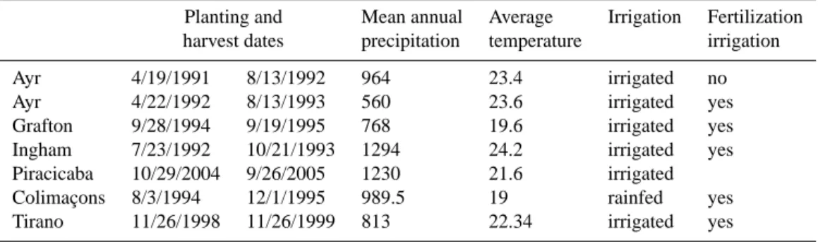
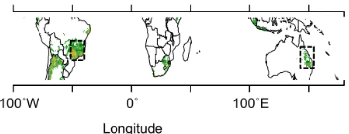
This study is based on sugarcane field trials in three regions (Fig. 2) where sugarcane is of economical importance, Brazil (1 site), Australia (4 sites), and La Réunion Island (2 sites). These sites, already used by Valade et al. (2013), span differ-ent climatic conditions and agricultural practices, as shown in Table 1, which makes them useful for our purpose to pro-vide continental-scale sugarcane yield uncertainty estimates. More details about the four sites from Australia and La Réu-nion can be found respectively in Keating et al. (1999), Mu-chow et al. (1994), Robertson et al. (1996) and in Martiné (unpublished). The site from Brazil is described in Marin et al. (2011). The sensitivity analysis of the yield spatial distribution to the model parameters is carried out for two continental-scale areas where sugarcane is cultivated at large scale. In Brazil, we consider the region encompassing partly the São Paulo and Mato Grosso states, and in Australia the sugarcane cultivation belt of the northeastern coast (Fig. 2).
2.2 Model and parameters considered
We use the agro-land surface model ORCHIDEE–STICS (Gervois et al., 2004) in a version that was already cali-brated for sugarcane for leaf area index at the same sites as used here (Valade et al., 2013). This model chains the crop model STICS with sugarcane specific phenology and man-agement with the generic process-based land surface model ORCHIDEE that can be applied either at a site, or on a grid for regional runs.
STICS (Brisson et al., 1998) is an agronomical model designed for site-scale operational applications, which de-scribes in detail the soil and crop processes associated with specific crop varieties and with management practices, such as aboveground biomass, and biomass nitrogen content, wa-ter and nitrogen content in the soil, yield, and root density. Yet, STICS is a generic crop model, because from a set of common equations it can describe a large number of crop species through specific parameterizations. Similarly, spe-cific vectors of parameters define crop cultivars. STICS has been validated for a variety of cropping situations (Brisson et al., 2003)
ORCHIDEE (Krinner et al., 2005) is a land surface model developed for global applications, standing now as the land surface model of the IPSL Earth System Model. It has been developed from the association of a surface energy and water balance scheme (SECHIBA) with a biogeochemistry module (STOMATE) and as such simulates the short timescale ex-changes of water and energy between the land surface and the atmosphere, as well as the processes of the carbon cy-cle including photosynthesis, respiration, carbon allocation, and soil decomposition. The vegetation is represented in OR-CHIDEE with the plant functional type (PFT) concept by grouping species into a few categories based on the simi-larities of their traits and resulting in an average plant. For example, sugarcane would fall in the generic “C4 crop” PFT in the standard version of ORCHIDEE, and this uncalibrated version of model fails to reproduce site-level phenology, as shown by Valade et al. (2013).
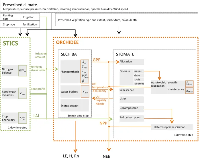
The chaining of STICS with ORCHIDEE was performed to improve the ability of ORCHIDEE to simulate specific crops, for which the PFT concept was not appropriate, as it lacks representation of crop phenology and crop manage-ment practices (Gervois et al., 2004). In the chain-like struc-ture (Fig. 3), STICS calculates phenology, water and nitro-gen requirements, and passes the key variables of leaf area index (LAI), root profile and nitrogen stress as well as the in-put data concerning irrigation requirements to ORCHIDEE that uses them to calculate carbon assimilation and alloca-tion, water balance, and energy-related variables. The one-way coupling between the two models can generate some inconsistencies, such as the soil status that is different be-tween ORCHIDEE and STICS. This type of inconsistency, inherent to the structure of the model, is considered as part of the structural uncertainty and is not covered in this study.
Screening
7 sites Morris methodUncertainty
7 sites LHS 50 parameters U(O) 17 parameters U(S) U(OS) 3 parameters 8 parametersOp?miza?on at seven sites
STICS ORCHIDEE STICS ORCHIDEE
Uncertainty
7 sites LHSU(O) U(S) U(OS) STICS ORCHIDEE STICS ORCHIDEE
Sensi?vity
2 regions LHS / PRCC STICS ORCHIDEE STICS ORCHIDEE STICS ORCHIDEEReduc?on of the ranges
Figure 1. Flowchart of the analysis carried out in this study. The first step is the separate screening for seven sites of the STICS and ORCHIDEE parameters. The selection of parameters obtained from the screening are then used for two uncertainty analysis, one with the same parameter ranges of variation as for the screening, the other with parameter ranges of variation constrained by the optimization of the model at seven sites. Each uncertainty analysis is decomposed in three parts, one including only ORCHIDEE parameters, one including only STICS parameters and one including parameters from both ORCHIDEE and STICS. Finally a sensitivity analysis is carried out for two small regions in Australia in Brazil for all parameters together.
Table 1. Description of climate and management for the sites used in this study in Australia (Ayr, Ingham, Grafton), Brazil (Piracicaba) and La Réunion (Colimaçons, Tirano).
Planting and Mean annual Average Irrigation Fertilization harvest dates precipitation temperature irrigation
Ayr 4/19/1991 8/13/1992 964 23.4 irrigated no
Ayr 4/22/1992 8/13/1993 560 23.6 irrigated yes
Grafton 9/28/1994 9/19/1995 768 19.6 irrigated yes
Ingham 7/23/1992 10/21/1993 1294 24.2 irrigated yes
Piracicaba 10/29/2004 9/26/2005 1230 21.6 irrigated
Colimaçons 8/3/1994 12/1/1995 989.5 19 rainfed yes
100˚W 0˚ 100˚E Longitude
Figure 2. Spatial distribution of the regions (dashed rectangles) used in this study overlaid on a map of the distribution of sugar-cane growing areas indicated in green.
However, this particular one-way structure will have a conse-quence in the uncertainty that we are analyzing in this study. ORCHIDEE and STICS each have a large number of pa-rameters involved at every step of a simulation over the course of a growing season. The values of these parameters – often empirically prescribed – are not easy to measure or are not measurable at all, calling in many cases for expert judgment to set their values, when it is impractical to find reference values. The uncertainty of these parameters is prop-agated onto the output variables of ORCHIDEE STICS and has impacts whose strength depends on the structure of both STICS and ORCHIDEE. Because of the chain-type struc-ture of ORCHIDEE–STICS (Fig. 3), the parameters from STICS that control LAI and nitrogen stress are expected to have a weaker and more indirect effect on downstream vari-ables, such as biomass compared with parameters from OR-CHIDEE that directly control carbon assimilation processes, and the development of biomass to produce yield at the date of harvest.
2.3 Parameter screening
In this section, we describe the screening step that allows us to select the most influential parameters upon which the model uncertainty is investigated. An initial set of 17 pa-rameters from ORCHIDEE and 50 papa-rameters from STICS is considered for the screening, according to their influence on the simulation of biomass production, based on expert knowledge and literature as listed in Table 2. The screen-ing analysis procedure is the same as described in Valade et al. (2013). It is based upon the method of Morris (Cam-polongo et al., 2007; Morris, 1991; Pujol, 2009) often used to explore the parameters space for complex models with a large number of parameters. Like all screening methods, the Morris method gives qualitative information on the sensitiv-ity of the output variables to the parameters, since it only discriminates parameters based on their importance, but does not provide information on the relative difference of impor-tance (Cariboni et al., 2007). Its aim is to reduce the dimen-sionality of the problem for further use of quantitative, com-putationally heavier methods (Saltelli et al., 2004).
The advantage of the Morris method is that it is compu-tationally efficient and easy to implement and interpret. It is based on a one-at-a-time approach, in which only one param-eter is changed between two runs, allowing for the calcula-tion of a local partial derivative of the output variable with respect to the input parameter, called an elementary effect. The Morris method is considered to be a “global” screening method, because the algorithm is repeated several times to calculate the elementary effects of each parameter in several locations of the parameters space, so that the average and standard deviation of all elementary effects associated with each parameter are representative of the behavior of this pa-rameter in its whole range of variation. The results of the Morris screening algorithm can be represented by a 2-D plot of standard deviation versus mean value of the elementary ef-fects on the output variable (here harvested biomass) of each parameter. A parameter with a high mean elementary effect (called µ, or µ∗ for mean of absolute values) is interpreted as a parameter with high influence on the output harvested biomass variable. A parameter with a high standard devia-tion of its elementary effects (σ ) is interpreted as inducing non-linearities in the model output, and/or as having interac-tions with other parameters.
Here, we apply the Morris method as implemented in the R “sensitivity” package (Pujol et al., 2013) using site-scale simulations of ORCHIDEE STICS across the seven field trial sites listed in Table 1. For each site, we identify the most influential parameters for the output variable harvested biomass. The parameters identified as important at least at two sites are selected for the rest of the study.
2.4 Uncertainty analysis (UA)
The goal of the UA is to quantify the overall uncertainty in the harvested biomass output variable that results from un-certain input parameter values. Firstly, based on the a pri-ori probability of each parameter’s value, a probability den-sity function is assigned to each parameter in order to gener-ate sample parameter sets according to the Latin Hypercube Sampling (LHS) method. Secondly, an ensemble of model runs is performed using those samples. Thirdly, the uncer-tainty on the output variables is obtained from the statistical properties of the distribution of simulated harvested biomass from the ensemble runs by defining the uncertainty as one standard deviation of the distribution.
The first step is thus to generate parameter samples con-strained with prior parameter ranges and statistical distribu-tions that are then used as inputs for ensemble simuladistribu-tions.
The parameters considered for the uncertainty (UA) for both STICS and ORCHIDEE are those selected by the screening analysis, allowing a reduction in the parameters space hypercube dimensionality and therefore in the re-quired computing resources. Starting from the initial set of 17 and 50 parameters, respectively, for the screening of OR-CHIDEE and STICS parameters, the Morris algorithm result
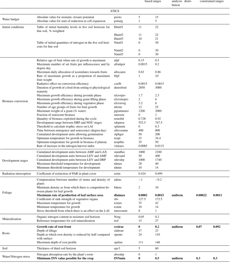
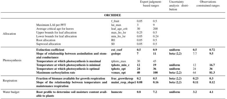
Table 2. List of parameters from STICS and ORCHIDEE included in each step of the analysis with their ranges of variation. Parameters in bold indicate parameters identified by the screening analysis as the most important for uncertainty propagation.
Expert judgment- Uncertainty Observations
based ranges analysis
distri-bution
constrained ranges
STICS
Water budget Absolute value for stomatic closure potential psisto 5 15
Absolute value for start of reduction in cell expansion psiturg 1 5
Initial conditions Table of initial humidity levels in five soil horizons for
fine soil, % weighted
Hinitf1 11 22
Hinitf2 11 22
Hinitf3 10 21
Table of initial quantities of nitrogen in the five soil hori-zons for fine soil
Ninitf1 0 30
Ninitf2 0 30
Ninitf3 0 30
Biomass conversion
Relative age of fruit when rate of growth is maximum afpf 0.15 0.5
Maximum number of set fruits per inflorescence and by degree day
afruitpot 0.0015 0.2
Maximum daily allocation of assimilates towards fruits allocamx 0.63 0.86
Rate of maximum growth as a proportion of maximum fruit weight
bfpf 1 10
Radiative effect on conversion efficiency coefb 0.0015 0.0815
Duration of growth of a fruit from setting to physiological maturity
dureefruit 2850 3000
Maximum growth efficiency during juvenile phase efcroijuv 1.7 2.3
Maximum growth efficiency during grain filling phase efcroirepro 2 6
Maximum growth efficiency during vegetative phase efcroiveg 3.2 6
Number of age groups of fruits for fruit growth nboite 12 25
Maximum weight of a grain (% water) pgrainmaxi 1200 2000
Fraction of senescent biomass ratiosen 0 1
Quantity of biomass exploited during the cycle remobil 0.728 0.92
Development range between DRP and NOU stages sdrpnou 552.5 747.5
Threshold to calculate trophic stress on LAI splaimin 0 0.3
Time between emergence and senescence (degree day) stlevsenms 400 800
Cumulated development units allowing germination stpltger 50 200
Optimum temperature for growth in biomass teopt 15 34.4
Optimum temperature for growth in biomass if plateau teoptbis 35 50
Rate of increase in the nitrogen harvest index vitirazo 0.0085 0.0115
Development stages
Cumulated development units between AMF and LAX stamflax 1000 2100
Cumulated development units between LEV and AMF stlevamf 50 400
Cumulated development units between LEV and DRP stlevdrp 1000 1740
Maximum threshold temperature for development tdmax 28 40
Minimum threshold temperature for development tdmin 10 14
Radiation interception Coefficient of extinction of PAR in plant cover extin 0.424 0.699
Foliage
Compensation between number of stems and density of plants
adens −1 −0.2
Minimum density as from which there is competition be-tween plants for leaf growth
bdens 2 10
Maximum rate of production of leaf surface area dlaimax 0.0002 0.0015 uniform 0.00022 0.0011
Coefficient of sink strength of vegetative organs sbv 127.5 172.5
Maximum temperature for growth tcmax 35 42
Minimum temperature for growth tcmin 10 14
Stress threshold from which there is an effect on the LAI tutressmin 0 1
Mineralization Organic nitrogen content in moisture soil horizon Norg 0.05 0.2
Reference temperature for soil mineralization tref 15 27
Roots
Growth rate of root front croirac 0 0.2 uniform 0.07 0.092
Depth of tillage zlabour 17 23
Depth at which root density is reduced by half compared with surface
zpente 24 110
Maximum depth of root profile zprlim 111 140
Soil Thickness of third soil horizon epc3 5 60
Water/Nitrogen stress Nitrogen absorption rate by the plant’s roots absodrp 0 1
Table 2. Continued.
Expert judgment- Uncertainty Observations
based ranges analysis
distri-bution
constrained ranges
ORCHIDEE
Allocation
f_fruit 0.05 0.5
Maximum LAI per PFT lai_max 3 9
Average critical age for leaves leaf_age_crit 30 200
Upper bounds for leaf allocation max_lto_lsr 0.25 0.5
Lower bounds for leaf allocation min_lto_lsr 0.05 0.24
Root allocation R0 0.05 0.5
Sapwood allocation S0 0.05 0.5
Photosynthesis
Extinction coefficient ext_coef 0.5 0.9 uniform 0.5 0.72 Slope of relationship between assimilation and
stom-atal conductance
gsslope 7 11 beta (2,2) 7.7 9.5 Temperature at which photosynthesis is maximal tphoto_max 30 45
Temperature at which photosynthesis is minimal tphoto_min_c 12 19 uniform 12 16.7 Temperature at which photosynthesis is optimal tphoto_opt 24 36 uniform 24 36 Maximum carboxylation rate vcmax_opt 40 100 beta (2,2) 64 81.3
Respiration Fraction of biomass available for growth respirationSlope of the relationship between temperature and frac_growthresp 0.2 0.5 beta (2,2) 0.23 0.3
maintenance respiration
maint_resp_slope1 0.08 0.16 beta (2,2) 0.11 0.12
Water budget Root profile to determine soil moisture content
avail-able to plants
humcste 0.8 7.2 uniform 3.2 4.1
(see Sect. 3.1) allows us to reduce the parameter numbers to 8 and 3 parameters for ORCHIDEE and STICS.
For the UA, we use Monte Carlo methods, which are com-putationally less expensive than variance-based approaches (Marino et al., 2008), making them a frequent choice in environmental sciences (Poulter et al., 2010; Verbeeck et al., 2006; Zaehle et al., 2005). The Monte Carlo sampling scheme used here is the stratified LHS, which is an efficient scheme for generation of multivariate samples of statistical distributions (McKay et al., 1979). In LHS, the range of each
of the k parameters X1, X2, . . . Xk included in the study is
divided into N intervals of equal probability. One value is randomly selected from each interval. The N values obtained
for the X1parameter are then paired at random, without
re-placement, with the N values obtained for the X2parameter,
then to the N values obtained for the X3parameter and so
on until the kth parameter. The procedure results in N sets of k parameters, or samples, that can be used for input to the model. In this study, from the 11 parameters identified by the screening, the N value is set to 250, resulting in 250 simula-tions for exploring the uncertainty around modeled biomass for each site.
In order to get insights on the part of the uncertainty at-tributable to each of the two models chained together, STICS and ORCHIDEE (Fig. 1), first, only the uncertainty com-ing from ORCHIDEE parameters is evaluated (Fig. 1), sec-ondly, only the uncertainty propagated from STICS param-eters (Fig. 1), and last, uncertainties propagated from both ORCHIDEE and STICS parameters are considered together through the chained model ORCHIDEE–STICS.
An important difficulty in the utilization of sampling-based UA methods is the lack of literature about a priori probability distribution of most parameters, given the depen-dency of output upon a priori assigned values (Marino et al., 2008). If most studies rely on a thorough literature search and expert judgment (Medlyn et al., 2005; Verbeeck et al., 2006; Wang et al., 2005), this approach might result in an over-estimation of the model output uncertainty due to combina-tions of extreme parameters values that are not realistic and therefore excessively decrease the estimated reliability of the models. Some studies have addressed this issue by trying to rationalize the parameter ranges through benchmarking out-puts (removing parameter sets resulting in values for output variables outside of a given benchmark range) or by prescrib-ing hypothesized correlations between parameters (Poulter et al., 2010; Zaehle et al., 2005). Here, after a first estimation of uncertainty based on expert opinion for the a priori pa-rameter range (overestimation of uncertainty), we propose a second approach to overcome the scarcity of information about parameter reference distributions by reducing the pa-rameters a priori range based on site-optimized values, thus providing narrower and more realistic a priori ranges that are constrained by observations (likely underestimation of un-certainty).
For the first a priori estimation of parameter range, ranges and distributions are assigned to parameters based on expert knowledge and previous parameterization studies (Kuppel et al., 2012) and centered on their a priori values. The a priori ranges prescribed using this approach are considered as overestimations of the likely ranges for parameters’ val-ues for sugarcane because they are adapted from studies in which parameters’ ranges were assigned for plant functional
Nitrogen) stress)index) Soil) Temperature) )&)humidity) Prescribed)climate) Temperature,)Surface)pressure,)Precipita<on,)Incoming)solar)radia<on,)Specific)humidity,)Wind)speed)
ORCHIDEE(
STICS(
STOMATE) SECHIBA) Photosynthesis) Water)budget) Energy)budget) Alloca<on) Biomass) Senescence) LiHer) Decomposi<on) Soil)carbon)pools) Heterotrophic)respira<on) Autotrophic) respira<on) LE,)H,)Rn) NEE) 30)min)<meMstep) 1)day)<meMstep) Prescribed)vegeta<on)type)and)extent,)soil)texture,)color,)depth) Crop)) phenology) Root)length) dynamics) Nitrogen)) balance) LAI) fer<liza<on) Crop)type) Plan<ng) date) Irriga<on) 1)day)<meMstep) GPP) LAI) Rugosity) Albedo) leaves) roots) stem) reserves) Root)profile) Irriga<on) amount) growth) maintenance) NPP) δLAI max κroot kext Tmin Topt VC max opt β κhum fGresp αMresp INNminFigure 3. Structure of the ORCHIDEE–STICS chain model. STICS calculates the crop phenology, water and nitrogen requirements and passes LAI, root profile, irrigation and nitrogen nutrition index to ORCHIDEE. ORCHIDEE consists in the coupling of two module. SECHIBA simulates the photosynthesis process, water and energy budgets; STOMATE is a carbon module and calculates carbon fluxes and to the atmosphere (respiration) and carbon accumulation in the carbon pools (biomass compartments, litter, soil).
types instead of a single crop, as is the case here, and some-times used for optimization studies, therefore requiring wide enough ranges within the model’s domain of applicability (Groenendijk et al., 2011; Kuppel et al., 2012). By using overestimated ranges for input parameters, we estimate an upper bound for the value of the uncertainty on output vari-ables.
The second (site-constrained) a priori estimation is a re-finement of the uncertainty estimation based on the idea that the “real” probability distribution of the parameters can be approached by the distribution of optimal parameters over all the possible case studies (sites, weather, management). It is of course not possible to determine the model’s opti-mal parameters for an infinite number of eco-climatic and land-management conditions, but a sample of representative case studies can provide a rough estimate of the parame-ters plausible range. Building on this hypothesis, the model is calibrated independently at seven sites using an iterative
method, seeking to constrain the uncertainty analysis with observation-based parameter ranges. For this, we performed a Bayesian calibration of the model parameters, using a stan-dard variational method based on the iterative minimization of a cost function that measures both the model data mis-fit as well as the parameters’ deviations from prior knowl-edge. The iterative scheme is described in Tarantola (1987) with the hypothesis of Gaussian error on the observations and the parameters. At each site, parameter values are var-ied iteratively until the best match between simulation and observation is found. More details on the calibration results can be found in the Supporting Information. We are aware that the optimization of the parameters at seven sites only to obtain a representative a priori range of the parameters distri-butions likely results in an optimistic estimate of this range even though the sites chosen cover different climatic, edaphic and management conditions, making them well suited for ap-plying our method. This observations-constrained range is
highly dependent on growing conditions. When the model is applied to the context of climate change, these ranges may then be out of their domain of significance and the first wider estimate of prior parameters distribution, based on literature, must be preferred.
For both a priori parameter range estimations (expert judg-ment vs. site constrained), when no parameter value appears to be more likely than another, a uniform a priori uncertainty distribution is prescribed. When there is some level of con-fidence that the a priori value is more likely, we use a beta distribution. This type of distribution is often used for un-certainty analyses, because of its adjustable shape (param-eterized equation) and advantage of having bounded tails (Monod et al., 2006; Wyss and Jorgensen, 1998). The suc-cessive analysis of both techniques provides an improve-ment in the estimation of the uncertainty from the first (expert-judgment based, likely too pessimistic) to the second (observation-based, perhaps too optimistic) approach.
2.5 Spatial sensitivity analysis (SA)
The first step in the sensitivity analysis also consists in gen-erating parameter samples. The same parameters are consid-ered for the SA as for the UA (Sect. 2.4), that is, the 11 pa-rameters (8 papa-rameters from ORCHIDEE and 3 papa-rameters from STICS) selected by the screening analysis.
As opposed to the UA where all parameters are consid-ered together for their effect on the distribution of the har-vested biomass output variable, the goal of the sensitivity analysis is to rank the influence of parameters based on their impact on the biomass and its spatial distribution obtained in
the continental-scale 0.7◦runs. The partial correlation
coeffi-cient (PCC) measures the correlation between an output vari-able and a parameter after the correlation with other parame-ters has been eliminated (Marino et al., 2008). However, for monotonic but non-linear relationships, these measures per-form poorly and a rank transper-formation needs to be applied to the data first to linearize the relationship. The correlation calculated between the rank-transformed data is then called partial rank correlation coefficients (PRCC). PRCC has been found to be an efficient indicator for the influence of param-eters, because it is a measure of the sensitivity of the out-put to parameters (Saltelli and Marivoet, 1990). The larger the PRCC, the more important the parameter is with respect to the output variable. Here, the relationship between mod-eled biomass on a grid, and parameters is diagnosed through the calculation of the partial ranked correlation coefficients (PRCC) on each grid point between the output and parame-ter, assuming a monotonic behavior of the model.
The SA is implemented from the results of the 0.7◦
simu-lations over Brazil and Australia (see Fig. 1 and Sect. 3.5). In this regional sensitivity analysis, ORCHIDEE–STICS is run for each region on a grid of 20 by 15 grid points and 13 by 20 grid points, respectively, driven by gridded climate forc-ing fields from the reanalysis products ERA-Interim (Dee et
al., 2011), with varying parameter values from a sampling where only bounds and no distributions were assigned to the parameters. The management information (date of planting, date of harvest, fertilization, irrigation) and the soil proper-ties (as described in Valade et al., 2013) are assumed to be uniform across each region and were defined as typical of each area. The a priori bounds used for the parameters in the SA correspond to the first version of the parameter ranges considered in the uncertainty analysis (i.e., derived from ex-pert knowledge). As cited by Wang et al. (2005), for sensitiv-ity analyses, Bouman (1994) advises using parameter ranges as broad as possible within the limits of the model valid-ity domain. Once the parameters’ a priori bounds have been set, ensemble runs are performed with all the parameter sets. From the distributions of input parameters and output vari-ables obtained at each pixel, a spatial distribution of PRCC is obtained, which is interpreted in Sect. 3.5 in terms of re-gional differences of each parameter on modeled sugarcane yield.
The interest of carrying out such a regional sensitivity analysis is that it provides maps of the geographic patterns of the importance of each parameter, leading to a better com-prehension of the mechanisms behind the parameter-related model sensitivity. These results can be very useful for plan-ning purposes, for instance when quantifying the different factors controlling sugarcane yield and ethanol production over a large region under future climatic conditions as com-pared to present-day conditions.
3 Results and discussion 3.1 Screening
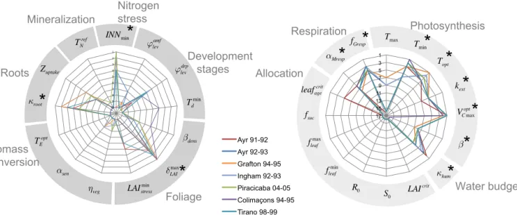
From the Morris screening method, we obtain for each pa-rameter two indices µ∗ and σ , that measure the influence of each parameter and its degree of involvement in non-linearities and interactions with other parameters, respec-tively. We first made sure that no parameter with a significant value for µ∗ was above the line σ = 2µ∗, which would im-ply that non-linearities and/or interactions would be so strong that the uncertainty propagation from the parameter to the model output could not be clearly established. None of our parameters selected for their significant values of µ∗ was above this line (Fig. S2 in the Supplement). From µ∗ and σ values, we establish a ranking of the parameters by only con-sidering parameters involved in limited interactions and/or non-linearities (σ < 2µ∗) and then we rank the remaining parameters based on their µ∗ index, a larger µ∗ being inter-preted as a more influential parameter. The Morris parame-ters ranks for ORCHIDEE and STICS are respectively shown in Fig. 5a and b, where each radar plot corresponds to one model. The axes refer to the parameters and the line colors to the sites. For STICS, for the sake of readability, not all of the initially selected 50 parameters are represented on the
VC max= VC max opt ⋅ε
temp⋅εwater⋅εleaf light= e−kext.LAI
κroot: root growth rate
fGresp : fraction of GPP lost as growth
respiration (dimensionless) Gresp=
1 Δt(fGresp⋅ Balloc) ci= max 0 ci 01+ α MrespTi ( ) ⎧ ⎨ ⎪⎪ ⎩⎪⎪ Mresp=Δt1 ci⋅ Bi i≠leaf∑ + cleaf⋅ Bleaf⋅ 0.3⋅ LAI +1.4 1− e( −k⋅LAI) LAI ⎛ ⎝ ⎜ ⎞⎠⎟
αMresp : slope of the dependance on
temperature of maintenance
respiration coefficient (K-1)
Tmin/ Topt : Minimum / Optimal
photosynthesis temperatures (°C) zroot eff= κ root. fΔT.pfz. fanox.dt 0 T ∫
εtemp= f T(air,Tmin,Topt)
gs : Stomatal conductance (µmol.m -2.s-1) hr : Air relative humidity (kg.kg
-1) Ca : Air CO2 concentration (ppm) VC max : Effective rate of carboxylation (µmol.m
-2.s-1) εtemp : Temperature limitation (unitless)
VC maxopt : Rate of carboxylation in
optimal conditions (µmol⋅m−2⋅s−1)
β : Ball-Berry slope (unitless)
εtemp : Limitation of photosynthesis capacity by temperature
kext : extinction coefficient (unitless) light : Light fraction that goes through the vegetation
ci : Fraction of biomass lost as maintenance respiration for part i (unitless)
ci0 : Prescribed maintenance respiration coefficients at 0 Degree Celsius (unitless)
Ti : Air (soil for belowground compartments) temperature (°C)
Mresp : Maintenance respiration (gC.m -2.dt−1) Bi : Biomass in compartment i (gC.m -2) gs= β hr Ca A+ gs offset δLAI
max : daily maximum increment
of LAI (m2.plt-1.deg-day-1)
d : Sowing density (plt.m-2)
αdens,βdens : Parameters describing competition from planting density(unitless, plt.m −2) Tcrop,Tcrop
min,T crop
max : Actual, minimum and maximum temperature for crop growth (°C) kLAI : LAI development stage (unitless)
LAI : Leaf area index (m2.m-2) INN,WS : Nitrogen nutrition index, water stress
CN crit,C
N
plt : Actual and critical nitrogen concentration in the plant (%)
splai : Stress index for competition between foliage and sugar accumulation (unitless)
A : Assimilation (µmol.m-2.s-1) gs
offset : Offset constant (unitless)
εstress : Water and nitrogen limitation (unitless)
εleaf : Limitation from leaf age (unitless)
Gresp : Growth respiration (gC⋅m2⋅dt-1) Balloc : Allocatable biomass (gC⋅m
2)
zrooteff : Depth of the root front efficient for absorption (cm)
fΔT : Minimum temperature for emergence of the crop (°C) pfz : Water status of the soil layer (unitless) fanox : Anoxia effect
LAI= ΔLAI dev⋅ Δ LAI T ⋅ Δ LAI dens⋅ Δ LAI stress.splai.dt 0 T ∫ ΔLAI dev= δLAI max 1+ ef k(LAI)
ΔLAIstress= min
INN= maxCN plant CNcrit , INNmin ⎛ ⎝⎜ ⎞ ⎠⎟ Ws ⎧ ⎨ ⎪ ⎩ ⎪ (Monsi and Saeki, 1953) (Krinner et al., 2005) (Ishida et al., 1999) (Ball et al., 1987) Tbg= 1 Kint + Tk⋅ e
−κhum⋅zk−1−e−κhum⋅zk
( ) k=1 nlay ∑ fw= αsat⋅e −κhum⋅htop+ 1−α sat ( )⋅e−κhum⋅hbottom
Tbg : Temperature for below-ground biomass (K)
Kint : Integration constant (unitless)
nlay, zk : Number of soil layers, depth of the kth soil layer (m)
Tk : Soil temperature for kth layer (K)
fw : Water fraction available for the plant (unitless)
αsat : Normalizing coefficient related to wetness of the top soil layer (unitless)
htop,hbottom : Depth of dry soil in the top and bottom layers (m) ΔLAI
dens= eαdenslog
d βdens ⎛ ⎝ ⎜⎜⎜ ⎜ ⎞ ⎠ ⎟⎟⎟ ⎟⎟⋅d Δ LAI T = Tcrop− Tcrop min if Tcrop≤ Tcrop max Tcropmax− T crop min if Tcrop≥ Tcrop max ⎧ ⎨ ⎪ ⎩⎪
INNmin: threshold for nitrogen
nutrition index (unitless)
ORCHIDEE STICS
κhum: Root profile description (m
-1 ) (Brisson et al., 2009) (Brisson et al., 2009) (Krinner et al., 2005; Ruimy et al., 1996) (Ruimy et al., 1996) (Krinner et al., 2005)
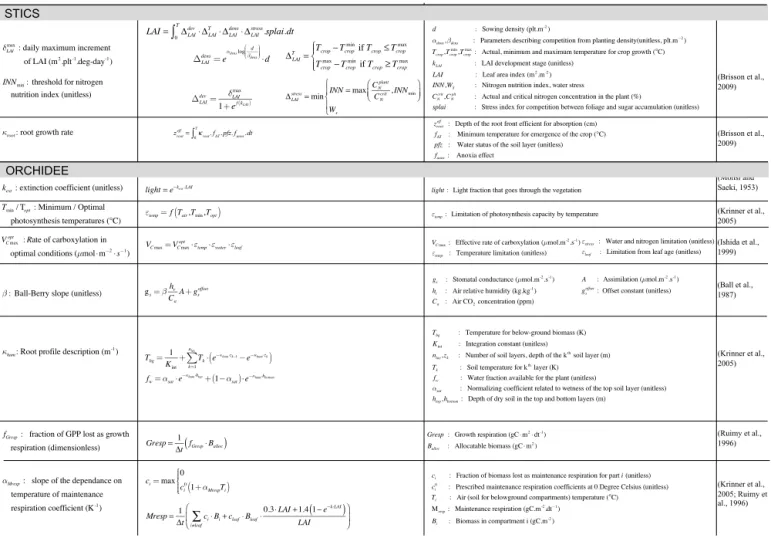
Figure 4. Main parameters for simulation of sugarcane yield with ORCHIDEE–STICS with the equations in which they are involved.
radar plot but only those parameters that pertain to the 10 top-ranked parameters at least at one site. The maximum number of 10 parameters was fixed based on examination of Morris indices µ∗ and σ at individual sites that only revealed 3 to 5 sensitive parameters each time. The positions and roles in the model of the parameters identified as most important are shown in Fig. 3. Figure 4 gives more details, with the main equations through which these parameters affect the output variables of STICS and of ORCHIDEE.
The three most influential parameters of STICS (Fig. 3a) reflect the way STICS and ORCHIDEE are chained (Fig. 3). Indeed, from the chained model structure, the indirect impact of STICS parameters on harvested biomass occurs through their effect on processes related to LAI, root growth and nitrogen stress, the only STICS variables passed to OR-CHIDEE for calculating biomass. This chaining of the mod-els through three variables is reflected in the identification of the three most important STICS parameters, which
con-trol the daily maximum rate of foliage production, δmaxLAI, the
growth rate of the root front, κroot, and the threshold of
nitro-gen nutrition index, INNmin. δLAImaxand INNminparameters are
both involved in LAI calculation. Indeed, the LAI equation
has four members describing four processes of the sugarcane
foliage development. First, the LAI development (1devLAI in
Fig. 4) describes the potential LAI increase through the scal-ing of the daily maximum rate of foliage production by a
function of the development stage (kLAI), and is logically
directly controlled by the value of parameter δLAImax. The
sec-ond member in the equation represents the temperature effect on LAI growth through the accumulation of degrees above a
temperature threshold (Tminin Fig. 3). The last two members
of the equation represent processes that can limit LAI devel-opment, competition for light between plants due to planting
density (1densLAIin Fig. 4) and a limitation from trophic stress
emerging from competition between plant components for nitrogen based on calculation of a nitrogen nutrition index
limited by parameter INNmin. The root growth rate κroothas
a less direct impact on LAI since it intervenes in the calcula-tion of the root front depth, which then impacts the availabil-ity of nitrogen and water and therefore the stress status of the
crop (impact on CNplantand Wsin Fig. 4).
The eight most influential parameters that control har-vested biomass in ORCHIDEE, are identical for all sites ex-cept at the Colimaçons site (where only seven parameters are
1" 2" 3" 4" 5" 6" 7" 8" 9" 10" 11" Aus_Ay_5" Aus_Ay_6_9293" Aus_Gr_11_1" Aus_In_3" Bre_Pi_i0405" Reu_Co_i95" Reu_Ti_i99" κroot αsen δLAI max TE opt ϕlev drp Zuptake INNmin ηveg Biomass conversion Nitrogen stress Roots Mineralization LAIstress min βdens Td min ϕlev amf Development stages Foliage TN ref 1" 2" 3" 4" 5" 6" 7" 8" 9" 10" 11" Ayr 91-92 Ayr 92-93 Grafton 94-95 Ingham 92-93 Piracicaba 04-05 Colimaçons 94-95 Tirano 98-99 leafage crit Tmax S0 R0 LAIcrit fsuc Topt β κhum αMresp fGresp Tmin fleaf min fleaf max kext VC max opt Photosynthesis Respiration Allocation Water budget 1 3 5 7 9 11 13 15 17 Total&biomass&above-ground& Ayr 91-92 Ayr 92-93 Grafton 94-95 Ingham 92-93 Piracicaba 04-05 "Colimacons 94-95" Tirano 98-99 1" 2" 3" 4" 5" 6" 7" 8" 9" 10" 11" Ayr 91-92 Ayr 92-93 Grafton 94-95 Ingham 92-93 Piracicaba 04-05 Colimaçons 94-95 Tirano 98-99
(a) STICS parameters
(b) ORCHIDEE parameters
*
*
*
*
*
*
*
*
*
*
*
Figure 5. Parameters rankings derived from the Morris screening analysis for STICS parameters (a) and ORCHIDEE parameters (b) for seven sites (color lines). Each axis of the radar plot corresponds to the rank of a parameter, the lower the rank, the more important the parameter.
identified as influential by the Morris method). The Morris top-ranked parameters of ORCHIDEE control photosynthe-sis and water budget equations as well as respiration pro-cesses (Fig. 4). Three of those (the minimum and optimal
temperatures for photosynthesis, Tmin, Topt, the maximum
rate of carboxylation VCmaxopt )directly affect the rate of
car-boxylation Vc that is calculated from the maximum rate of
carboxylation weighted by a mean leaf efficiency and scaled by a limiting factor depending on the optimum and mini-mum temperatures for photosynthesis. The stomatal
conduc-tance gs that links assimilation and transpiration is defined
by the Ball–Berry equation (Ball et al., 1987) as a function of assimilation and depends on the air relative humidity and
CO2concentration, scaled by a slope factor, called the Ball–
Berry slope (β). The root profile constant (κhum)describes
the exponential distribution of root density in the soil and is involved in the definition of available water and root
tem-perature. Finally, the extinction coefficient (kext)intervenes
in an equation derived by Monsi and Saeki (1953), similar to Beer’s law, which describes the attenuation of light with depth in the canopy.
Two ORCHIDEE parameters controlling autotrophic res-piration also stand out, with the maintenance resres-piration
co-efficient (αMresp) and the fraction of biomass allocated to
growth respiration (fGresp). The leafcritageparameter that is
in-volved in the biomass allocation also ranked high (fifth most important) but only for one site and is therefore not retained for the rest of the study.
For the chained model ORCHIDEE–STICS, the 11 most influential parameters show a good agreement between sites for the most important parameters as seen in Fig. 5 where ranking lines overlap for most of the parameters. Building on the results of the Morris screening analysis, we select the eight top-ranked parameters for ORCHIDEE and three for STICS that were revealed as influential for biomass for fur-ther uncertainty and sensitivity analysis.
3.2 Uncertainty analysis: parameters controlling biomass uncertainty at a typical site
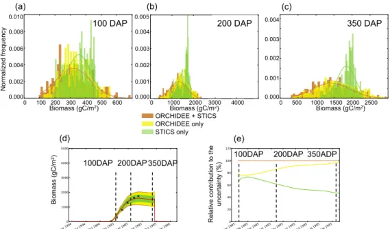
In this section, we attribute the harvested biomass uncertainty to the uncertainty of the ORCHIDEE vs. STICS parameters. The simulated biomass uncertainty is a function of time dur-ing the growdur-ing season, and it differs between sites. In Fig. 6, we show the contributions of ORCHIDEE and STICS pa-rameters, respectively, to the total uncertainty for one typical site, Grafton, Australia, during the 1994–1995 growing sea-son, which has climate conditions within the range of other sites. Figure 6a–c display the normalized frequency distri-butions of simulated biomass obtained from ensemble runs for three times in the growing season: (1) very early in the cycle in Fig. 6a, at 100 days after planting (DAP), (2) dur-ing the peak growdur-ing season in Fig. 6b, at 200 DAP and (3) shortly before harvest in Fig. 6c, at 350 DAP. We dis-tinguish between the normalized frequency distributions of simulated biomass when considering the uncertainty prop-agated from STICS parameters alone (green), ORCHIDEE parameters alone (yellow), and from ORCHIDEE and STICS parameters together (brown), along with their best-fit normal
ORCHIDEE + STICS ORCHIDEE only STICS only (a) (c) R el at ive co nt rib ut io n to th e un ce rt ai nt y (% ) (d) Biomass (gC/m2) Biomass (gC/m2) N orma lize d fre qu en cy 100DAP 350DAP 100 DAP (e) 350 DAP Bi oma ss (g C /m 2) 200 DAP (b) 200DAP Biomass (gC/m2) 350ADP 100DAP 200DAP 100 200 300 400 500 600 0.010 0.008 0.006 0.004 0.002 0.000 0 0.005 0.004 0.003 0.002 0.001 0.000 1000 2000 3000 4000 0 0.004 0.000 0.003 0.002 0.001 0 500 1000 1500 2000 2500
Figure 6. Uncertainty analysis for the site Grafton 94–95. (a–c) Probability distributions of harvested biomass simulated after parameter uncertainty (from STICS: green, from ORCHIDEE: yellow, from ORCHIDEE+STICS: brown) has been propagated into the model. (d) Reference simulation of harvested biomass (red) and uncertainty from ORCHIDEE, STICS, ORCHIDEE+STICS. (e) Contribution (%) of ORCHIDEE (yellow) and STICS (green) to the total uncertainty (brown) over the length of the growing season.
distributions overlaid. These distributions were obtained by Monte Carlo LHS ensemble runs (Sect. 2.4) with a sampling of parameters of STICS alone, ORCHIDEE alone and of both models together. We consider uncertainties starting from the
time when biomass reaches 50 gC m−2 in order to discard
the emergence phase during which biomass is very low and uncertainties are therefore not significant.
At 100 DAP (Fig. 6a), the uncertainty distribution of biomass related to ORCHIDEE parameters U(O) spans a slightly larger range than the distribution related to STICS, U(S), and it has more extreme values. The U(O) distribution is symmetrical around the mean value, with a standard
devia-tion of 86.9 gC m−2. The U(S) distribution is non-symmetric,
skewed towards larger values of biomass, and it has a slightly
smaller standard deviation (76.5 gC m−2)than that of U(O).
Combining U(O) and U(S) in Monte Carlo runs by vary-ing the parameters of both models at the same time gives the total uncertainty distribution, U(O+S), shown in brown in Fig. 6. This distribution has more extreme values and a
higher standard deviation (112.0 gC m−2), in other words,
U(O+S) > U(O) + U(S).
At 200 DAP (Fig. 6b), and later at 350 DAP (Fig. 6c), the picture has changed. First, all uncertainty distributions are wider than at 100 DAP. Secondly, the means of U(O) and U(S) are no longer in agreement, with the asymmetric U(S) distribution being even more shifted towards high val-ues of the harvested biomass. The reason for this shift is that among the variables transmitted from STICS to ORCHIDEE in the chain of models, the only one that can act to increase the biomass calculated by ORCHIDEE in the later phase of
the growing season, near 350 DAP, is LAI. This is because a higher LAI will result in increased photosynthesis and there-fore biomass in ORCHIDEE. However, past a certain thresh-old, the LAI impact saturates when the foliage is sufficient for all incoming light to be captured, and therefore, uncer-tainty on the STICS parameters that impact LAI will not in-crease the uncertainty of biomass any longer. Unlike LAI, the nitrogen stress and root profile variables controlled by the parameters of STICS continue to act as limiting factors on biomass throughout the peak and late growing season. The saturation of the biomass uncertainty associated with STICS parameters is stronger at 200 DAP than at 300 DAP, when biomass increase has slowed down and the role of LAI for driving biomass is less important.
In Fig. 6d, the total uncertainty U(O+S) is given for the reference simulation (with parameters at their maximum likelihood values, red line) and the uncertainty on harvested biomass can be defined as a percentage of the harvested biomass in the reference simulation. For the Grafton site, at harvest, the overall uncertainty is 26 %. The relative contri-butions of ORCHIDEE and STICS to the total uncertainty,
αO and αS, respectively, are defined by αO=U(O+S)U(O) , αS=
U(S)
U(O+S). The evolution of these contributions to the total
un-certainty is shown in Fig. 6e. We can see in this example that U(O) > U(S) during the entire growing season, but with a de-crease of U(S), and an inde-crease of U(O) such that the inde-crease in biomass uncertainty seen in Fig. 6d becomes increasingly dominated by uncertain ORCHIDEE parameters. The pro-gressive increase in the weight of ORCHIDEE parameters
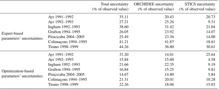
Table 3. Uncertainty associated with STICS, ORCHIDEE, or ORCHIDEE+STICS parameters uncertainties expressed as percentage of the reference harvested biomass for each site and for each of the two uncertainty analysis.
Total uncertainty ORCHIDEE uncertainty STICS uncertainty (% of observed value) (% of observed value) (% of observed value)
Expert-based Ayr 1991–1992 35.11 20.43 20.73 parameters’ uncertainties Ayr 1992–1993 27.21 25.26 9.31 Ingham 1992–1993 38.60 31.42 21.04 Grafton 1994–1995 26.05 23.92 14.07 Piracicaba 2004–2005 25.49 23.36 14.00 Colimaçons 1994–1995 41.21 41.87 18.61 Tirano 1998–1999 44.26 36.80 30.61 Optimization-based Ayr 1991–1992 31.20 14.01 25.64 parameters’ uncertainties Ayr 1992–1993 15.84 15.60 4.58 Ingham 1992–1993 21.66 22.35 9.19 Grafton 1994–1995 16.84 15.25 9.81 Piracicaba 2004–2005 14.67 14.80 5.84 Colimaçons 1994–1995 21.31 20.01 10.28 Tirano 1998–1999 22.26 18.06 15.03
uncertainties is due to the reduction in the role played by LAI for biomass increase along the growing season. Indeed, if early in the season the foliage is crucial to allow photosynthe-sis and carbon allocation, later in the cycle, other processes become important as well; past a certain LAI for which all incoming light is captured, it might not even play a role any-more, and then the STICS parameters only impact biomass accumulation through nitrogen stress index and root depth.
3.3 Uncertainty analysis: role of ORCHIDEE vs. STICS parameters in controlling biomass uncertainty at seven sites
Table 3 summarizes the results of the overall parametric uncertainty analysis at the seven sites, including Grafton. The total uncertainty U(O+S) ranges between 25.5 % of biomass at Piracicaba, Brazil during 2004–2005 and 44.26 % of harvested biomass at Tirano, La Réunion in 1998–1999. This yields an average uncertainty on biomass at harvest (due to uncertain parameter values of the chained model ORCHIDEE–STICS) of 34.0 % of harvested biomass across the seven sites, in the order of previous results on different variables in similar studies using process-based models, such as Dufrêne et al. (2005) who found an uncertainty of 30 % on modeled NEE for forest sites in France with the CASTANEA model.
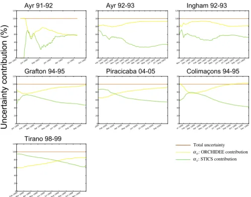
As for the ORCHIDEE vs. STICS relative contributions to the uncertainty of simulated biomass at all sites, the re-sults at each site are not identical but display a similar gen-eral pattern shown by Fig. 7. For all sites, the ORCHIDEE parameters contribution to total uncertainty increases dur-ing the cycle, or remains approximately constant for Ing-ham in 1992–1993, and increases during the growing cycle to dominate entirely the total uncertainty at the end of the
cycle compared to STICS parameters. The STICS contribu-tion to overall uncertainty decreases during the growing sea-son to reach a minimum by the end of the growing seasea-son. For sites Piracicaba during 2004–2005, Tirano in 1998–1999 and Colimaçons during 1994–1995, during the beginning of the cycle the U(S) is even larger than U(O). The results for Ayr in 1991–1992 display a less clear pattern. Indeed, at the end of the cycle, the contributions of ORCHIDEE and STICS to the total uncertainty are almost equal, due to an in-crease in STICS contribution during the second half of the cycle. This result confirms a hypothesis made in Valade et al. (2013) where the difficult calibration of LAI at this site was attributed to the simulation by STICS of an important stress. Indeed if a large stress is simulated by the pheno-logical module, this can impede ORCHIDEE processes of biomass growth and therefore increases the weight of STICS parameters with respect to ORCHIDEE ones.
3.4 Uncertainty analysis: constraining uncertainty from site optimization
Optimizing the 11 ORCHIDEE–STICS parameters selected from the screening analysis at seven sites leads to a re-duction of the width of the a priori uncertainty distribu-tion of the parameters (Table 2). Carrying out the same un-certainty analysis with a narrower unun-certainty range of pa-rameters (thanks to their site calibration) leads to an im-portant reduction of uncertainties of biomass, both for the STICS and ORCHIDEE components of uncertainty. This can be seen by comparing Fig. 6 (initial range of parameters) with Fig. 8 (narrower range after parameter calibration at the sites). For site Grafton during 1994–1995 for example, U(O+S) gets reduced from 26 % to 17 % for the reference harvested biomass, U(O) from 24 % to 15 % and U(S) from
Ayr 91-92 Ayr 92-93 Ingham 92-93
Grafton 94-95 Piracicaba 04-05 Colimaçons 94-95
Tirano 98-99 Total uncertainty αO: ORCHIDEE contribution αS: STICS contribution
U
nce
rt
ai
nt
y
co
nt
rib
ut
io
n
(%
)
Figure 7. Contribution (%) of ORCHIDEE (yellow) and STICS (green) to the total uncertainty (brown) over the length of the growing season for seven sites.
14 % to 10 %. Figure 9 and Table 3 (bottom section) show the uncertainty contributions and overall uncertainty estimates for the seven sites after observation-based reduction of the a priori uncertainty on parameters. The overall parametric un-certainty of biomass defined as the 1-sigma standard devia-tion of the (O+S) distribudevia-tion has thus been reduced to 21 % on average, to 11.48 % when attributed to STICS alone, and to 17.15 % when attributed to ORCHIDEE alone (Table 3).
The ORCHIDEE and STICS contributions to the total un-certainty keep the same general pattern as with the initial pa-rameter uncertainty distribution, with a domination of OR-CHIDEE parameters in the uncertainty towards the end of the growing season (Fig. 9). Compared with the first uncertainty budget with expert-based parameters uncertainties (Fig. 8), there is generally a slight decrease in the STICS contribution at the end of the season.
We have thus established full uncertainty budgets for the two components of the ORCHIDEE–STICS chain of mod-els, which has revealed variations in the uncertainty in the biomass simulation from site to site. The next step is to dis-criminate between the different parameters the ones that con-tribute most to the overall uncertainty through a sensitivity analysis at regional scale.
3.5 Spatial sensitivity analysis: sensitivity of sugarcane yields to the model parameters for Brazil and Australia
The overall parametric uncertainties have been quantified at seven sites and attributed to either STICS or ORCHIDEE. The sensitivity analysis (SA) in this section will go a step further and leads to discriminate the different parameters that contribute to the spatial distribution of uncertainty over the two regions considered. This sensitivity analysis is per-formed at regional scale because from the previous section, we have seen that the uncertainty in the biomass simulation varies from site to site.
Ensemble runs at regional scale were conducted over Brazil and Australia, each with different value combinations for the 11 parameters previously selected through the Morris screening analysis (Table 1). The Partial Rank Correlation Coefficients (PRCC) were then calculated for each pixel in each of the two regions (see Sect. 2.5), and the SA results are discussed for two dates during the growing season, 200 and 350 days after planting (DAP). The SA results express the strength of the relationship between an uncertain param-eter and the simulated biomass at harvest at each pixel. The statistical significance of the PRCC calculated for each grid cell is tested with the associated p values, and non-significant PRCC are removed (p value < 0.05). The first date, 100 DAP, examined for site-scale UA studies (Sect. 2.3) is not shown here, because no statistical significance was found in the cor-relations between the parameters and the harvested biomass
ORCHIDEE + STICS ORCHIDEE only STICS only Bi oma ss (g C /m
2) 100DAP 200DAP 350ADP
R el at ive co nt rib ut io n to th e un ce rt ai nt y (% )
100DAP 200DAP 350DAP
(a) (c)
100 DAP 200 DAP 350 DAP
(b) N orma lize d fre qu en cy Biomass (gC/m2) Biomass (gC/m2) Biomass (gC/m2) (d) (e) 0.012 0.014 100 200 300 400 500 600 0.010 0.008 0.006 0.004 0.002 0.000 0 0.005 0.004 0.003 0.002 0.001 0.000 1000 2000 0 0.004 0.000 0.003 0.002 0.001 0 500 1000 1500 2000 2500 500 1500 2500
Figure 8. Uncertainty analysis for the site Grafton 94-95 after parameter uncertainty ranges have been constrained through optimization at seven sites. (a–c) Probability distributions of harvested biomass simulated after parameter uncertainty (from STICS: green, from OR-CHIDEE: yellow, from ORCHIDEE+STICS: brown) has been propagated into the model. (d) Reference simulation of harvested biomass (red) and uncertainty from ORCHIDEE, STICS, ORCHIDEE+STICS. (e) Contribution (%) of ORCHIDEE (yellow) and STICS (green) to the total uncertainty (brown) over the length of the growing season.
Ayr 91-92 Ayr 92-93 Ingham 92-93
Grafton 94-95 Piracicaba 04-05 Colimaçons 94-95
Tirano 98-99 Total uncertainty αO: ORCHIDEE contribution αS: STICS contribution U nce rt ai nt y co nt rib ut io n (% )
Figure 9. Contribution (%) of ORCHIDEE (yellow) and STICS (green) to the total uncertainty (brown) over the length of the growing season for seven sites after parameter uncertainty ranges have been constrained through optimization at seven sites.
at 100 DAP. Then, the pixels’ statistically significant PRCC, calculated for each parameter, can be analyzed both in a ge-ographical projection (latitude, longitude) (Figs. 11 and 12, columns 1–2 and 4–5) and in a (temperature, precipitation)
climatic space projection (Figs. 11 and 12, columns 3 and 6). The regional sensitivity analysis thus carried out for sugarcane-growing areas in Brazil and Australia shows the magnitude, spatial distribution and climatic dependency of