AN ALGORITHM FOR
PARALLEL UNSTRUCTURED MESH
GENERATION AND FLOW ANALYSIS
by
Tolulope 0. Okusanya
B.Sc. Mechanical Engineering Rutgers University, New Jersey, 1994SUBMITTED TO THE DEPARTMENT OF AERONAUTICS AND ASTRONAUTICS
IN PARTIAL FULFILLMENT OF THE REQUIREMENTS FOR THE DEGREE OF
MASTER OF SCIENCE at the
Massachusetts Institute of Technology February 2, 1996
@Massachusetts Institute of Technology 1996 All Rights Reserved
Signature of Author
Department of Aeronautics an/ Astronautics
-ebruary 2, 1996
Certified by I ---
-Professor Jaime Peraire, Thesis Supervisor Department of Aeronautics and Astronautics
Accepted by
Professor #tarold Y. Wachman, Chairman Department Graduate Committee
;:ASACHUSJ TS: S NS'i'T U'TE
OF TECHNOLOGY
FEB
211996
PARALLEL UNSTRUCTURED MESH GENERATION
AND FLOW ANALYSIS
by
Tolulope O. Okusanya
Submitted to the Department of Aeronautics and Astronautics on February 2, 1996
in partial fulfillment of the requirements for the degree of Master of Science in Aeronautics and Astronautics
Abstract
A strategy for the parallel generation of unstructured meshes is proposed. A distributed unstructured mesh generation environment is presented and this is cou-pled with a time dependent compressible Navier-Stokes equations solver. The mesh generation schemes developed in the serial context are extended for parallel execution. Dynamic load-balancing and mesh migration are incorporated to ensure even work dis-tribution and for refinement analysis. Anisotropic mesh refinement is also incorporated for flow analysis involving anisotropic gradients. The flow solver is linked to the mesh generation environment as a test of the parallel mesh generation capabilities for flow analysis and several well defined test cases are modeled for comparison to experimental results.
Acknowledgements
First of all, I would like to thank my thesis advisor, Professor Jaime Peraire for his invaluable support and encouragement over the past year. He has shown me new and interesting views and was always a constant source of ideas. I look forward to working
with him in the future and wish him the best in his new role as a father.
A very special thanks goes to Dr. Andrea Froncioni and Professor Richard Peskin who started me off in the field of CFD. It was a real pleasure working with them at Rutgers. Here is to "Andy" in the hopes of his settling down long enough for a few bouncing baby bambinos.
Thanks goes to all my friends at CASL, GTL and SSL who have moved on and are still here. To those who endured the nightmares of taking the qualifiers and/or writing a thesis, pray you do not have to do such again. Things would simply not be the same without mentioning Folusho, Karen, Graeme, Ray, Jim, Carmen, Guy (Go RU !), Angie, Ed and K.K. (Remember guys, that was no ordinary chicken !!). Ali deserves special mention because like it or not, our fates are tied together somehow.
I also wish to thank the "arcade" group (that's right, you know yourselves !) espe-cially the other members of Team Megaton Punch for at least dragging me out of the lab (kicking and screaming) to go have fun. What would life have been without hearing phrases like "Feel the power little guy"?
Of course, I wish to thank my parents for their unconditional love and support without which I would never have been here in the first place. Lastly, I wish to thank God because there is only so far you can go by yourself.
%tctU
Ui: ttU
9
MP\®
0n
Sq
a
U4rI
cz
IC-T
Hakai no Tenshi0)
f1'
Contents
1 Introduction
1.1 Overview . . . .
2 Mesh Generation Algorithms
2.1 Prelim inaries .. ... ... ... .. ... ... ... ... ... .. ...
2.1.1 Delaunay Triangulation ...
2.1.2 Constrained Delaunay Triangulation . . .. . . . . .
2.2 Delaunay Triangulation Algorithms . . . .
2.2.1 Watson Point Insertion Algorithm . . . .
2.2.2 Green-Sibson Point Insertion Algorithm . . . .
2.2.3 Alternative Point Insertion Algorithms . . . .
2.3 Implementation Issues ...
2.3.1 M esh Control ...
2.3.3 Geometric Searching ...
2.4 Mesh Generation Process ...
2.4.1 Preprocessing ...
2.4.2 Interior Point Creation ...
3 Anisotropic Grid Generation Extension
3.1 Anisotropic Refinement ...
3.2 Wake Path Generation ...
4 Parallel Systems and Model Overview
4.1 Parallel System s ...
4.1.1 SIM D architecture ...
4.1.2 MIMD architecture ...
4.1.3 Shared Memory Systems ...
4.1.4 Distributed Memory Systems ...
4.2 Distributed memory programming model . . . .
5 Parallel Automatic Mesh Generation
5.1 Introduction . .. . . . . 31 32 36 37 40 43 43 43
5.2 Previous Efforts ...
5.3 Requirements ...
5.3.1 Data Structure ...
5.4 Parallel Grid Generation ...
5.4.1 Element Migration . .
5.4.2 Load Balancing ....
5.4.3 Element Request .. .
5.4.4 Procedure ... ... ... .. ... ... ... ... ... .. ...
6 Grid Generation Results
6.1 Mesh Migration Results ...
6.2 Load Balancing Results ...
6.3 Mesh Generation Results ...
7 CFD Application 7.1 Pream ble . . . . 7.2 Governing Equations . . .. 7.3 Non-Dimensionalization ... 7.4 Spatial Discretization ... . . . . 52 . . . . 55 . . . . 60 . . . . 70 . . . . . . 89
7.4.1 Interior Nodes .
7.4.2 Boundary Nodes . . . .
7.5 Artificial Dissipation . . . .
7.6 Temporal Discretization . . . .
7.7 Boundary Conditions ...
7.7.1 Wall Boundary Conditions . . . .
7.7.2 Symmetry Boundary Conditions . . .
7.7.3 Farfield Boundary Conditions . . . . .
7.7.4 Boundary Layer Boundary Conditions
7.8 Parallelization ...
7.8.1 Edge Weight Parallelization . . . .
7.8.2 Parallel Variable Update . . . .
7.9 Results . . . .
8 Conclusions
A Mesh Generation Function Set
B Parallel Communication Function Set
100 100 100 101 . . . . 101 102 102 103 106 107 109
C Element Migration Algorithm
D Partition Location Algorithm
Bibliography
111
112
List of Figures
2.1 Watson Point Insertion Strategy . . . .
2.2 Edge Swapping with Forward Propagation . . . .
2.3 Source Elem ent ...
2.4 Point, Line and Triangle Sources ...
2.5 Rebay Point Insertion Algorithm ...
2.6 Non-manifold mesh example ...
3.1 Viscous Flat Plate Mesh ...
3.2 Anisotropic Refinement Parameters . . . .
3.3 Anisotropic Point Creation ...
3.4 Viscous Mesh Generation on 737 Airfoil . . . .
3.5 Trailing Edge Closeup of 737 Airfoil ...
3.6 Wake Path Generation on NACA-0012 Airfoil . . . .
4.1 Possible connectivities for Shared Memory MIMD systems .
4.2 1D, 2D, 3D and 4D hypercube connectivity . . . .
4.3 3D torus connectivity . . . .
5.1 Interprocessor Front Segment . . . . .
5.2 Element Migration Philosophy . . . .
5.3 Element Migration Example . . . .
5.4 Linear 1D Load Balance System . . .
5.5 Remote Element Request Configuration Example . .
5.6 Constrained Triangulation Violation . . . .
5.7 Cyclic Ring Deadlock ...
5.8 Green-Sibson Element Configuration Exception . . .
5.9 Slave Processor Operation ...
6.1 Mesh Migration Throughput ...
6.2 Load Balancing Results for Random Element Assignment ...
6.3 Mesh Generation of 1 Million Elements . . . .
6.4 2D Parallel Mesh Generation -Four processor illustrative example . . . . . . . . 46
. . . . . 54
. . . . . 56
7.1 Interior Node Control Volume . . . .
7.2 Edge Weight Vector ...
7.3 Boundary Point Control Volume . . . .
7.4 Single Layer Halo ...
7.5 Mach Number Contours for Supersonic Bump . . . .
7.6 Mach Number Contours for Flat Plate . . . .
93 94 95 103 ... . 104 105
List of Tables
List of Symbols
Q Computational domain
Qk Global element k (Serial)
Sfj,k Local element k in subdomain
j
(Parallel)Rd Computational dimension
{Vi} Voronoi regions for point set {xi}
Rf Rebay factor
Si Minimum distance from point i to boundary
0 Minimum anisotropic refinement spacing
rg Anisotropic geometric growth ratio
Gf Growth limiter factor
N, Number of processors
Tj Global element identification tag
Q Migrated element set
cm Contiguous subset of migrated element set
nB Number of X bands
nyB Number of Y bands
GNe Global number of elements
GNP Global number of vertices
GNpf Global number of processor fronts
Bx,[i] Required average number of elements in X band (i)
{ir}
Nr {Fr} {F"} p P u, v E H FG 7 Pr Re c TTXX, Tyy, TXY, TYX
WX , wY, W, -Wy Sp At CFL Sf F.F(vi)
Initial element set before remote element request Final element set after remote element request Number of remote request processors
Granted remote element set for request transfer Initial front set before remote element request
Final front set after remote element request Pressure Density 2D velocity components Total energy Total enthalpy State vector Flux components Ratio of specific heats Prandtl number Reynolds number Local speed of sound Local temperature
2D stress components Viscosity coefficient Edge based weights Pressure switch Local time step
Courant-Friedrichs-Lewy condition Safety factor
Chapter 1
Introduction
1.1
Overview
Unstructured mesh methods for computational fluid dynamics have experienced a rapid growth over recent years and, for the computation of inviscid flows, have achieved a considerable level of maturity. As a result, a number of systems incorporating automatic mesh generators and flow solvers have been built which are currently being used in a semi-production mode by industry and research establishments [21, 25, 40]. The main advantage of the unstructured mesh approach is that, for complex geometries, it allows to significantly reduce the time period associated with the CFD analysis cycle. This feature is especially valuable during the early stages of design of aircraft when a large number of options needs to be analyzed.
The reasons for distributed mesh generation are twofold. The first one is to re-duce the computational times required for mesh generation. Currently, the serial mesh generator within the unstructured mesh system FELISA [25] generates grids at an ap-proximate constant rate of 3 million elements per hour on a high end workstation. It is conceivable that for the large grids required for viscous turbulent flow analysis, mesh generation may become a problem. More important however, are the memory require-ments. At present, the size of a computation is determined by the ability to generate the grid on a serial machine. For large applications, the memory requirements can be a
problem. For instance, the generation of an unstructured grid containing 8 million cells requires a serial machine with 512Mb of core memory using the FELISA system [25] . Once generated, this grid needs to be partitioned and sent to the parallel processors to carry out the flow solution. Hence, a strategy capable of generating a grid in parallel mode and such that when the grid generation process is finished, the grid is already partitioned and in place for the flow solution, is necessary.
This thesis addresses the development of a parallel unstructured mesh generator designed to operate on parallel MIMD machines with distributed memory. Serial mesh generation is a prerequisite to any form of parallel mesh generation since this is essen-tially mesh generation on a single processor. The serial mesh generation algorithms are detailed in chapter 2 and these deal with the algorithms, data structures and mesh representation. Chapter 3 deals with the extension of isotropic mesh generation to anisotropic mesh generation for analysis involving anisotropic gradients. Parallel sys-tems based on architecture and memory organization is discussed in chapter 4. This chapter also discusses the programming model adopted for the purpose of parallel mesh generation. The development of a parallel mesh generation system is discussed in chap-ter 5 and this deals with the topics of mesh migration, load balancing and the parallel extension of the serial mesh generation algorithms. The results of the serial and par-allel mesh generation systems are presented in chapter 6. The mesh generation system can only be truly tested under an actual CFD application and the formulation of an explicit 2D compressible Navier-Stokes equation solver is presented in chapter 7. The results for several test configurations is presented in this chapter with conclusions and recommendations for future work in chapter 8.
Chapter 2
Mesh Generation Algorithms
2.1
Preliminaries
A general description of a computational mesh in Rd may be given as a set of unique global coordinate vertices, {xi I i = 1..M} along with some form of connectivity in-formation regarding this set of points. Computational grids can be broadly subdivided into two major classes: structured and unstructured although mixed or hybrid grids also exist. Structured meshes in general do not require the connectivity information as this may be deduced from the point set distribution. Unstructured meshes require this con-nectivity due to the lack of a logical structure to the point set distribution. This may be thought of in the sense that the number of connectivity paths meeting at a point varies from point to point. The meshes considered here will be such that the connectivity information associated with any given grid satisfies the following constraints.
* The connectivity information is contained in a set of closed polyhedral elements
k which span the domain.
* Any given pair of polyhedral elements in Rd may share up to n global points.
* Any given set of (d-1) points which are coplanar and form an element face can be shared by at most two elements. In the case of boundary faces, these are shared by exactly one element for external boundaries and possibly two elements for internal
boundaries.
Given this set of constraints, we observe that the polyhedral elements (tfk) have been defined in a way such that for any given domain fl, the elements satisfy
S= U nk (2.1)
k
which implies that the elements are non-overlapping and tile the entire domain. The polyhedral elements considered for grid generation are triangles in 2D and tetrahedra in 3D.
2.1.1 Delaunay Triangulation
A triangulation of a given set of points in Rd may be effected by means of Dirichlet
tessellation. The Dirichlet tessellation of a point set {xi} is defined as the pattern of
convex regions {Vi} which is formed by assigning to each point xi, a region Vi which represents the space closer to point xi than any other point. These regions satisfy the property
V
= x:
{
x-
x
<
Ix- xjl}
Vj
i
(2.2)
The resultant convex polyhedra are called Voronoi regions and cover the entire domain. The Delaunay triangulation of a point set is then formed by considering any point pair with a common Voronoi boundary segment and joining them together. This results in a triangulation of the convex hull of the point set {xi} and is also referred to as the dual of the Voronoi diagram of the point set.
If Delaunay triangulation is considered in R2
, we observe that since each line seg-ment of the Voronol diagram is equidistant from the two points it separates, then each
vertex of the Voronoi diagram must be equidistant from the three nodes which form the Delaunay triangle that encloses the vertex. This is to say that the vertices of the Voronoi diagram are the circumcenters of the Delaunay triangles. In R3, this translates to the vertices of the Voronoi diagram being the circumcenters of the Delaunay tetrahedra.
The Delaunay triangulation satisfies a number of properties in R2 not all of which have extensions to R3. These include
1. Completeness. The Delaunay triangulation covers the convex hull of all points.
2. Uniqueness. The Delaunay triangulation is unique except for degeneracies such as 4 or more cocircular points (in R2) and 5 or more cospherical points (in R3).
3. Circumcircle/ Circumsphere criteria. A triangulation of N points is Delaunay if and only if every circle passing through the three vertices of a triangle in 2D (sphere passing through the four vertices of a tetrahedra in 3D) does not contain any other point.
4. Edge circle property. A triangulation of N points in 2D is Delaunay if and only
if there exists some circle passing through the endpoints of every edge which is point-free. This can be extended to 3D for element faces.
5. Equiangularity property. The Delaunay triangulation of a given set of points max-imizes the minimum angle of the triangulation. Hence the Delaunay triangulation is also called the MaxMin triangulation. This only holds in R2.
6. Minimum Containment Circle(Sphere). The Delaunay triangulation minimizes
the maximum containment circle(sphere) over the entire triangulation. The con-tainment circle(sphere) is defined as the smallest circle(sphere) enclosing the ver-tices of a triangle(tetrahedron).
7. Nearest neighbor property. An edge formed by connecting a vertex to the nearest
neighbor is always an edge of the Delaunay triangulation.
8. Minimal roughness. Given an arbitrary set of data fi defined on the vertices of the mesh such that fi varies as a piecewise linear function over the elements. For every possible triangulation, the Delaunay triangulation minimizes the functional
I = J Vf.Vfd (2.3)
2.1.2 Constrained Delaunay Triangulation
For a given point set {xi
I
i = 1..M}, the boundary of the Delaunay triangulation ofthe point set is the convex hull of the point set. However, if the Delaunay triangu-lation of a point set with respect to a prescribed set of fixed edges which bounds the domain is considered, this is referred to as a Constrained Delaunay triangulation. This prescribed set of edges may represent the domain boundary or interior boundaries. In most practical applications, we will be interested in constrained triangulations.
2.2
Delaunay Triangulation Algorithms
For the purposes of mesh generation, Incremental Insertion algorithms are considered. These algorithms are designed in such a way that given a point set, the points are considered in sequence and inserted into the triangulation in such a way as to ensure that the grid is always locally Delaunay. Due to the localized nature of these algorithms, global Delaunay cannot always be guaranteed. Several incremental insertion strategies exist such as the Bowyer algorithm [1] and Randomized algorithms [30]. However for the purpose of computational simplicity, we consider only the Watson algorithm [12]
and the Green-Sibson algorithm [43]. These are outlined in 2D but are extendable to 3D.
2.2.1 Watson Point Insertion Algorithm
The Watson point insertion strategy is based on the circumcircle property of the De-launay triangulation. Given a point Q to be inserted into the current triangulation, the
root element is defined as any element whose circumcircle contains the point. From the
root element, a Breadth First Search (BFS) is performed to locate all elements whose circumcircle contains the given point. The BFS is a tree search which is accomplished by checking the neighbors of all the currently identified elements which violate the cir-cumcircle test and considering only those elements which have not been tested. This may be done recursively or with the help of supporting data structure and is always guaranteed to terminate. This generated set of elements is always independent of the element selected as root. This search method is particularly suited to constrained tri-angulations where an element may not be visible to the point Q due to a prescribed edge. For constrained triangulations however, one required modification is to make sure that the root element is on the "same" side of the prescribed edge as the point Q by testing if the centroid of the root element is on the "same" side as Q. Deletion of the
set of elements which violate the circumcircle condition results in a polygonal cavity surrounding the point Q. This cavity is then retriangulated by connecting the point Q
to the vertices of the polygonal cavity. This guarantees that the triangulation is always locally Delaunay around the point Q. The implementation steps of the algorithm are listed below.
2. Locate root element with circumcircle containing point.
3. Perform tree search to obtain element set which violates circumcircle property.
4. Construct polygonal cavity edges and delete element set.
5. Connect cavity vertices to point Q and update Delaunay data structure.
This is the most general form of implementation for a given point set. In the process of mesh generation with constrained Delaunay triangulation, due consideration must be given to boundary violations also. Hence new points which are to be inserted into the triangulation are only inserted if there are no boundary or proximity violations with respect to the identified element set associated with the point Q. Proximity violations as defined in this context means that the new point Q may not be closer to any existing vertex than some specified tolerance.
2.2.2
Green-Sibson Point Insertion Algorithm
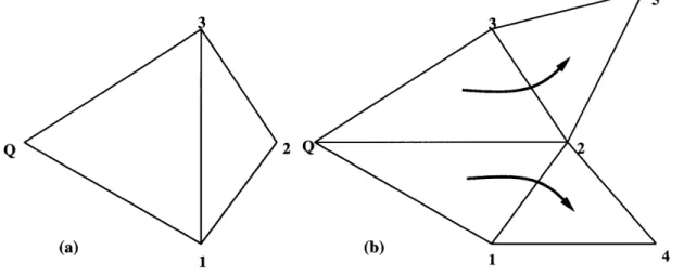
The Green-Sibson point insertion strategy is based on the circumcircle property of the Delaunay triangulation. The difference is that local edge transformations (edge swapping) are employed to reconfigure the triangulation. Given the point Q to be inserted into the triangulation, the root element is defined as the element that encloses the point Q. Upon the location of the root element, three new edges and elements are created by connecting Q to the vertices of the root element and deleting the root element. If the point lies on an edge, the edge is deleted and four edges are created connecting the point Q to the vertices of the quadrilateral formed. For the purpose of computational simplicity in mesh generation, if the point lies on an edge, then it is moved by small AL along the normal to the edge into the root element. Based on
Q
2
(a) (b)
1 1 4
Figure 2.2: Edge Swapping with Forward Propagation
the circumcircle criteria, the newly created edges will be Delaunay. However, some
of the original edges have now been rendered invalid and such, all edges which are termed suspect must be located. This is done by considering a "suspect" edge as the diagonal of the quadrilateral formed from the two adjacent elements. The circumcircle
test is applied to either of the adjacent elements such that if the fourth point of the quadrilateral is interior to the circumcircle, then the edge is swapped. This creates two more "suspect" edges which need to be tested. The process terminates when all the "suspect" edges pass the circumcircle test. The nature of the Delaunay triangulation guarantees that any edges swapped incident to Q will be final edges of the Delaunay triangulation. This implies that forward propagation [55] need be considered as depicted in figure 2.2. This may be done recursively or with the help of a stack data structure. The implementation of the algorithm is listed below.
1. Insert new point Q into existing point set.
2. Locate root element which encloses point.
3. Insert point and connect to surrounding vertices.
4. Identify "suspect" edges.
5. Perform edge swapping on "suspect" edges failing circumcircle test and identify new "suspect" edges.
6. If new "suspect" edges, go to Step 4.
As mentioned before, the problems associated with constrained Delaunay triangulation must also be considered with this method.
2.2.3 Alternative Point Insertion Algorithms
The primary point insertion algorithms implemented are as described above. However, it is sometimes necessary to generate non-Delaunay triangulations based on other criteria.
To this effect, we consider a modification of the Green-Sibson algorithm such that the circumcircle test is replaced by other criteria. Possible options are
1. Minimization of mazimum angle. This is referred to as a MinMax triangulation and considers the maximum angle for both the unswapped and swapped edge configuration. If the maximum angle for the swapped configuration is less than that of the unswapped configuration, the edge is swapped.
2. Minimization of skewness. This is referred to as a MinSkew triangulation which attempts to minimize the skew parameter for an element. The skewness parameter as defined by Marcum [13] is proportional to the element area divided by the circumcenter radius squared in 2D and to the element volume divided by the circumcenter radius cubed in 3D.
2.3
Implementation Issues
A number of issues need to be addressed for the implementation of the mesh generation algorithms outlined above. These are directly related to the problems associated with mesh control, data structure formats and geometric searching.
2.3.1 Mesh Control
Mesh control mechanisms must be included in mesh generation implementations to allow for control over the spatial distribution of points such that a grid of the desired density is produced. This can be accomplished by means of a background mesh and a source
Background mesh
A background mesh, implemented as tetrahedral elements in both 2D and 3D, is pro-vided such that desired mesh spacings are specified at the vertices of the elements. The background mesh must cover the entire domain and is defined such that the mesh spac-ing (or element size distribution) at any point in the domain interior is computed by linear interpolation on the background element which encloses the point. This provides a convenient method of specifying linearly varying or constant mesh spacings over the entire domain.
Source distribution
For complex geometries, specification of a background mesh can lead to a large number of background elements. This can be remedied by specifying sources at specific regions in the computational domain.
26-
1
- -
--Xc
D
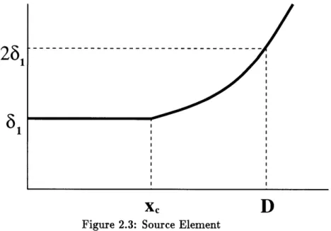
Figure 2.3: Source Element
which is a function of the distance from a given point to the source. The functional form of the mesh spacing specified by a point source is given by
61
6(x)
=
lepresented by where the mesh parameters are represented by
if x
<
zXif x > xc
1. x,: Distance over which mesh spacing is constant. 2. 61: Constant mesh spacing over distance x,.
3. D: Distance at which mesh spacing doubles.
P x
S
Point
(2.4) S %Triangle
Line
Figure 2.4: Point, Line and Triangle Sources
The sources may take the form of point, line or triangle sources as depicted in figure 2.4. The mesh spacing is defined for line and triangle sources as the spacing based on the closest point on the line segment or triangle This point is chosen as a point source with the mesh parameters x,, 61 and D linearly interpolated from the nodal values on the line or triangle source. Hence for any given point in the computational domain, the spacing is given as the minimum spacing defined by all the source spacings and that specified by the background mesh.
2.3.2 Data Structures
The choice of data structures to be employed in the mesh generation implementation plays an important role due to the nature of the algorithms. Efficient, compact and well structured data types are to be used to ensure fast execution. Some of the data structures as presented in L6hner [46] and Morgan [29] were implemented. The primary data structures involved include
1. Boundary Information: The constrained Delaunay triangulation involves a prescribed set of boundary edges. The information regarding a boundary edge is stored in a data structure termed a front segment which is to be distinguished from the front in regards to the Advancing Front Method for mesh generation e.g [25]. A front segment contains the information regarding the vertex identification indices (VID) of the boundary edge vertices, the attached element and any other marker information regarding the edge.
2. Element Adjacency: Element adjacency or neighbor information is also stored and explicitly updated. This involves increased memory usage but greatly reduces computation time. For a given front segment attached to an element, the element adjacency is modified to take this into account.
3. Dynamic Heaps: Several point creation algorithms used to determine the coor-dinate of the next generated point make use of some geometric property (such as the circumcircle radius or element area) of the current elements to generate the point. This usually involves some sort of sorting of the elements to find the seed element from which the point is to be generated. The Heap Sort algorithm [11, 50] was chosen due to the Q(log N) efficiency for insertion and deletion operations.
2.3.3 Geometric Searching
The problem of determining the members of a set of n points or elements in Rd which lie inside a prescribed subregion or satisfy some proximity criteria is known as geometric searching. Several algorithms involving O(log N) operations have been put forward [24, 23, 33] to solve this problem and other equivalent problems. The selected algorithm is the Alternating Digital Tree (ADT) algorithm which is an extension of the binary tree search methods. It provides for a fast and efficient method to perform geometric searches as presented in [22]. Examples of the use of ADT include point, edge and face proximity searches and root element location as in the case of the Green-Sibson point insertion algorithm.
2.4
Mesh Generation Process
Before the actual mesh generation can proceed, a preprocessing stage is necessary. Hence, the mesh generation process is divided into two phases with the preprocessor phase separate and taking place independent of the actual mesh generation.
2.4.1 Preprocessing
The mesh generation procedure begins with a geometric description of the computational domain f2 based on CAD/CAGD geometric models. The bounding curves and surfaces of the domain are modeled by creating a geometric description based on Ferguson cubic splines and bicubic patches [18]. The curve segments are discretized based on the mesh spacing specified by the background mesh from which the surfaces are created. The point creation schemes which are to be considered require an initial triangulation of the
computational domain. This is performed as described in [55].
2.4.2
Interior Point Creation
The mesh generation aspect involves the actual determination and creation of mesh ver-tex coordinates. This is a sequential procedure for the generation of new points in the domain based on some geometric property of the current triangulation and subsequent insertion based on the constraint imposed by the physical boundary edges. Several schemes have been put forward and are currently implemented in the literature. These include such algorithms as the Advancing Front Algorithm [25] and Circumcenter Al-gorithm [41]. In this work, three different alAl-gorithms have been implemented and these are outlined briefly below.
Rebay
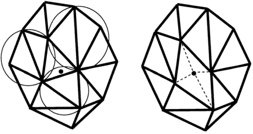
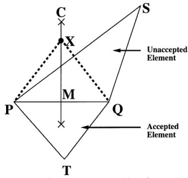
This algorithm as proposed by Rebay [53] is a variant of the Advancing Front algorithm which combines aspects of the Advancing Front algorithm with those of the Bowyer point insertion algorithm. The algorithm considers the division of the created elements into two groups which are tagged accepted and unaccepted. The accepted elements consist of those whose circumradii is less than a factor multiple (Rebay Factor Rf) of the desired element size defined as the mesh spacing at the circumcenter of the element. The algorithm proceeds by considering the maximal non-accepted element, defined as the element with the largest circumradius, which is adjacent to an accepted element as shown in figure 2.5.
The Voronoi segment which joins the circumcenters of the two elements is perpen-dicular to the common face between the two elements. The new point X is then inserted
on the Voronoi segment in the interval between the midpoint M of the common face and the circumcenter C of the non-accepted element. In the 2D context, let p be half the length of the common edge PQ and q be the length of CM. Given the desired circumcircle radius fM and defining
R = min max(fM, p), 2- (2.5) Rebay's algorithm inserts the new point X on the interval between M and C at a distance of
d = R + (R2 - p2) (2.6)
It is proven by Baker [54] that in 2D, the elements in the interior tend to equilateral triangles with possible distortions on the boundary.
C
S
/* - Unaccepted Element P 4 Accepted ElementFigure 2.5: Rebay Point Insertion Algorithm
Circumcenter Algorithm
This is a relatively fast and inexpensive algorithm which has been reported by Chew [42] and Ruppert [26]. The algorithm considers the maximal element defined as above and
generates the new point X at the circumcenter of the element. Chew proved that the elements generated by this algorithm have a minimum bound of 300 except for boundary effects.
Centroid Algorithm
This is another relatively fast and inexpensive algorithm reported by Weatherhill [41] which also considers the maximal element defined as above and generates the new point at the centroid of the element.
All the above considered point generation algorithms allow for a constrained trian-gulation with respect to the domain boundary edges. A common feature between them is that they consider the maximal element. This implies that the elements need to be sorted. This is the reason why a heap sort algorithm was implemented with supporting dynamic heap data structure. The mesh generation process simply consists of point creation and insertion until there are no more elements in the dynamic heap to con-sider. The facilitation of the entire mesh generation process may be done by having each point creation algorithm define a specified set of functions which will be invoked during execution such that any of the given algorithms may be chosen at will. This is implemented by currently defining a data structure of functions as in Appendix A. This function set is sufficient within the serial mesh generation context to provide enough functionality for any of the point creation algorithms.
Mesh generation systems for unstructured grid must be able to deal with the above mentioned issues. One issue which has not been mentioned is support for meshes gen-erated on non-manifold models. In a non-manifold representation, the surface area around a given point on a surface might not be flat in the sense that the neighborhood
of the point need not be a simple two dimensional disk. An example of such a mesh is shown in figure 2.6.
Chapter 3
Anisotropic Grid Generation Extension
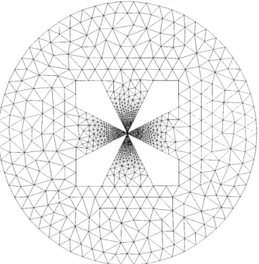
This chapter discusses the extension of the presented isotropic mesh generation al-gorithms to anisotropic meshes. Such meshes are required for many applications such as the computation of viscous flows which exhibit anisotropic gradients. The quality of the mesh in the regions of sharp gradients has to be such that the solution features are resolved. This may be done by increased refinement in the desired regions in an isotropic manner but this leads to a large number of elements. An alternative is to consider stretched triangulations in these regions as shown in figure 3.1 used for viscous flow calculation about a flat plate.
3.1
Anisotropic Refinement
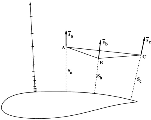
Anisotropic grids are produced by refining an existing initially isotropic grid [55]. This is based on the Steiner triangulation which is defined as any triangulation that adds additional points to an existing triangulation to improve some measure of grid quality. The stretching or refinement criteria is based on the minimum Euclidean distance S from the interior vertices of the elements to the boundary segments which have been marked for refinement as depicted in figure 3.2.
sa . IC
/
'B I Sb I II IFigure 3.2: Anisotropic Refinement Parameters
For each boundary curve which has been marked for refinement, two parameters o0 and r9 which represent the minimum spacing and the geometric growth ratio are
specified. A dynamic heap structure is maintained which sorts the "active" elements according to the minimum Euclidean distance of their vertices. An active element is
I I I I I I I I ISa I I I I I I
defined as one which has at least one vertex from which a new point can be generated. For each vertex in the triangulation, a unit vector - from the closest point on the closest boundary segment to the vertex is computed. The element measure chosen which determines if an element is active or not is based on the maximum dimension of the element projected along the vector s at the vertices of the element. For each vertex on an element, consider the element edges attached to that vertex. If the projection of any of the edge vectors along the unit vector ' associated with that vertex is larger than the specified spacing at the vertex, then the element is classified as active.
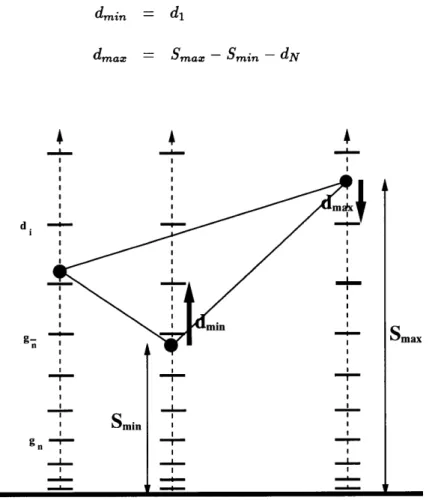
The candidate Steiner points associated with an active element are obtained at the vertices which correspond to the maximum and minimum Euclidean distances Smax and Smi, for the element. At the maximal vertex, a new point Xma, is inserted at a distance
dma,, along the unit normal Sa,, associated with the vertex and away from the closest boundary segment point. At the minimal vertex, a new point Xmin is inserted at a distance dmi, along the unit normal smin associated with the vertex and towards from the closest boundary segment point. This is as depicted in figure 3.3. The generation distances are chosen such that positions of the new points coincide with the points at which a point would have been created based on the geometric growth associated with the boundary segment such that the new points are created in uniform layers over the boundary segment. The procedure follows the following form
1. Given the current active element, the distances Smin and Sm,, for the element and 60 and rg for the closest boundary segment are obtained.
2. Generate distances based on the geometric growth sequence
until
fl-I
n - Smin > Gfborg' -1 (3.2) where Gf represents a growth limiter factor usually taken to be 0.5.
3. Generate set of N distances di based on geometric growth starting from gf until the condition below is satisfied.
Smax - di < Gfborgi+f- 1 (3.3)
The distances dma, and dmin are computed from these N generated distances using
dmin = di dmax d fi g Smin = Smax - Smin - dN (3.4) (3.5)
I
II
IrI
I
II
II
-r I Ic r I II I I I I I I 1 I I I I I r r I I I SmaxFigure 3.3: Anisotropic Point Creation
The candidate Steiner points are inserted into the triangulation only if there exists
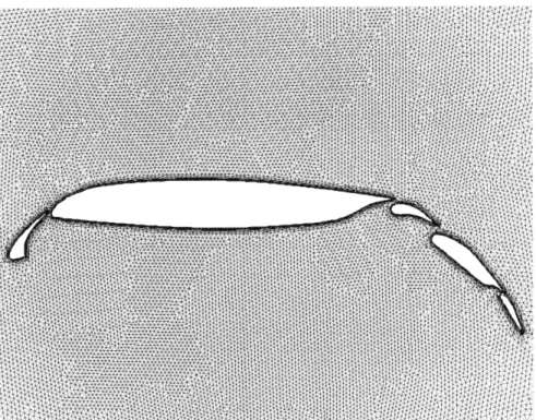
no other point in the triangulation which lies at a distance closer than the generation distance (dmax or dmin) associated with that point. The proximity query is performed by making use of the ADT structure of the current element set. The refinement is guaranteed to converge since a point is reached for all the elements such that either every element is refined or the geometric growth thickness at any point is greater than the mesh spacing at that point. Figures 3.4 and 3.5 show a mesh generated about a 5 element Boeing 737 airfoil by this strategy in which the minimum wall spacing was specified at 0.001% of the chord length.
3.2
Wake Path Generation
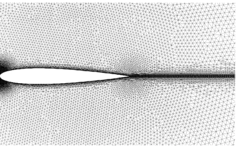
In viscous flow computations about airfoils, the wake path which is created by the airfoil is a region of interest. To properly resolve this region, the above technique may also be applied to create a stretched triangulation of the wake path.
To perform this, an initial guess must be made for the shape of the path. It should be noted that the procedure described here takes place in the preprocessing stage of the mesh generation. The wake path is initially modeled by making use of Ferguson cubic splines and discretized based on the background mesh. The discrete points on the wake path are inserted into the boundary triangulation. After insertion, the wake segments are treated as physical boundaries for subsequent constrained triangulation. After the isotropic mesh is generated, the Steiner triangulation proceeds as described above.
Figures 3.6 and 3.7 show the effect of wake path generation. The figures show a generated mesh about a NACA-0012 airfoil with both wake path generation and boundary refinement.
Figure 3.4: Viscous Mesh Generation on 737 Airfoil
Figure 3.6: Wake Path Generation on NACA-0012 Airfoil
Chapter 4
Parallel Systems and Model Overview
4.1
Parallel Systems
The last few years have witnessed a marked shift in the scale and complexity of problems which have been simulated numerically. This is due in part to the increased technology which has enabled significant advances in both computer software and hardware. How-ever, despite these improvements, numerous problems exist today which cannot still be solved with conventional uniprocessor computers. This is where supercomputers and parallel machines come into play and provide a chance at actually solving some of these problems.
The architectural classification of modern parallel systems falls into two major classes based on instruction execution and data stream handling.
4.1.1 SIMD architecture
The SIMD acronym stands for Single Instruction, Multiple Data and describes systems which are composed of a large number of (simple) processing units, ranging from 1K up to 64K, such that all may execute the same instruction on different data in lock step. Hence, a single instruction manipulates several data items in parallel. Examples of such systems include the MasPar MP-2 and the CPP DAP Gamma. It should be noted that
the SIMD architecture was once quite successful and is quickly disappearing. This is due in part to applications relevant to this type of architecture such as image processing, which is characterized by highly structured data sets and data access patterns.
Another subclass of SIMD systems are Vector processors and these incorporate special hardware or vector units which perform operations on arrays of similar data in a pipelined manner. These vector units can deliver results with a rate of one, two -and in special cases - three per internal clock cycle. Hence, from the programmer's point of view, vector processors operate on data in an SIMD fashion when executing in vector mode. Some examples of these systems in use include the Cray Y-MP, C90, J916 and T90 series and the Convex C-series.
4.1.2 MIMD architecture
The MIMD acronym stands for Multiple Instruction, Multiple Data and describes sys-tems composed of (relatively) few number of processors executing different instructions independently, each on an independent localized data set. In general, the incorporated hardware and software for these systems are highly optimized so that the processors can cooperate efficiently. Examples of such systems include the Cray T3D and the IBM SP2. The majority of modern parallel systems fall under this class. The full specifica-tions and descripspecifica-tions of current and some past systems may be found in [57]. Parallel systems, in particular the MIMD based systems, may also be classified based on the organization of memory.
4.1.3 Shared Memory Systems
Shared memory systems are characterized by all the processors having access to a com-mon global memory. Hence it is possible to have all the processors operating on the same common array, though care has to be taken to prevent accidental overwrites. As discussed in [57], the major architectural problem is that of connection of the proces-sors to global memory (or memory modules) and to each other. As more procesproces-sors are added, the collective bandwidth to the memory should ideally scale linearly with the number of processors, Np. Unfortunately, full interconnectivity is expensive, requir-ing O(Np2) connections. Hence a number of creative alternative networks have been
developed as shown in figure 4.1.
01234567 0 2 3 I 4 (a) n 5
Shared Memory System 6
7
CPU - - - - - CPU CPU Out
0 0 2 12 Network 3 3 4 4 5 5 6 6 Memory 0 0 2 2 3 n 3
(a): Crossbar (b): 0 -network (c): Central Databus (c) 4 m 4
5 5
6 6
7 7
Figure 4.1: Possible connectivities for Shared Memory MIMD systems
The crossbar network makes use of exactly N 2 connections and f network makes use of Np log2 Np connections, while a central bus represents only one connection. Due
to the limited capacity of the interconnection network, share memory parallel computers are not very scalable to a large number of processors. The
0 network topology is made
use of in such commercial systems as the IBM SP2.4.1.4 Distributed Memory Systems
Distributed memory MIMD system consist of a processor set {P I i = 1..Np} each with
its own local memory interconnected by a communication network. The combination of a processor and its local memory is often defined as a processor node such that each processor node is actually an independent machine. The communication between the processor nodes may only be performed by message passing over the communication network. The communication network for distributed memory systems is also of im-portance. Full interconnectivity is not a feasible option, hence the processor nodes are arranged in some interconnection topology.
Hypercube Topology
The hypercube nCUBE series.
d= 1
topology is a popular choice and is incorporated in such systems as the The hypercube topology as shown in figure 4.2
d=2
d=3 d=4
Figure 4.2: 1D, 2D, 3D and 4D hypercube connectivity
of links between any two nodes (network diameter) is d. Hence, the diameter grows logarithmically with the number of nodes. Also, several other topologies such as rings, trees, 2-D and 3-D meshes may be mapped unto the hypercube topology since these are all subsets of the hypercube topology.
Torus Topology
The torus or mesh topology is implemented on such systems as the Cray T3D and the 3D analog is shown in figure 4.3
Figure 4.3: 3D torus connectivity
The torus topology for a given dimension essentially consists of a periodic processor array which exhibits "wrapping". The rationale behind this is that most large-scale physical simulations can be mapped effectively on this topology and that a richer inter-connection structure hardly pays off.
Multi-Stage Topology
Multi-stage networks such as the
ft
network shown in figure 4.1 are characterized by small numbers of processor nodes connected in clusters with each cluster connected to other clusters at several levels. It is thus possible to connect a large number of processor nodes through only a few switching stages. Multi-stage networks have the advantage that the bisection bandwidth can scale linearly with the number of processors while maintaining a fixed number of communication links per processor. The bisectionbandwidth of a distributed memory system is defined as the bandwidth available on
all communication links that connect one half of the system (- processors) with the second half.
The major advantage of distributed memory systems over shared memory systems is that the architecture suffers less from the scalability problem associated with the connectivity bandwidth. However, the major disadvantage is that the communication overhead incurred in message passing is significantly higher. Another problem may occur if the system is not heterogeneous (i.e the individual CPUs are not identical) such that mismatch in communication and computation speeds may occur.
Due to the clear overall advantages of the distributed memory model and the MIMD architecture, this was the choice for the programming model for the implementation of the parallel grid generation system. A general comparison based on performance of several benchmarking tests on several distributed memory MIMD systems is given by Bokhari [52].
4.2
Distributed memory programming model
The distributed memory programming or message passing model is characterized by each processor node having its own local memory. Hence data which resides off-processor can only be accessed by having the processor on which the data resides send the data across the network. The implemented programming model is SPMD (Single Program, Multiple Data) in which one program is executed across all the processors executing on different parts of the same data set. This implies that the data must be distributed across the processor set. This partitioning is the basis of the parallel grid definition.
Implementation of message passing systems implies the existence of a communication library. The basic operation of the communication routines is data passing between ar-bitrary processor nodes and possibly the ability to check for the existence of messages in the message buffer. Higher level operations involve global operations such as broadcast-ing in which one processor node sends the same message to all other nodes, global sum, global minimum and global maximum of distributed data, and also global synchroniza-tion between a subset or possibly all of the nodes. In general, most distributed MIMD systems come with a native communication library usually written in C or FORTRAN such as on the IBM SP2 (MPL) or the nCUBE (NCUBE). A number of commercial efforts have been made to develop machine independent communication libraries and these include PVM [59], MPI [14], PARMACS [45] and CHARM [31].
The program structure is based on a message driven slave/master paradigm which allows for a highly concurrent implementation of the procedures involved. Other than the two operations of dynamic load balancing and work allocation, the slave processors are relatively independent of the master processor. Hence this model does not present a bottleneck. Based on the design philosophy of portability to distributed memory
MIMD systems, a communications library to provide a common interface for message passing has been developed for several major systems and is still undergoing additions. This library contains a base set of standard parallel communications routines which are outlined in Appendix B. This set of routines provide a minimal base of functions which enable a standard interface to parallel communication. Due to the peculiar nature of the distributed system, the parallel send and receive routines are blocking as opposed to
non-blocking. A blocking operation does not return control to the processor until the
message has been fully sent or received. However, options exist for specifying a non-blocking mode. Currently, this library has been implemented for the nCUBE and IBM SP2 native communication libraries as well as for the PVM and MPI message passing libraries.
Routines for operations which need to take place in a global fashion are also provided. These routines include
* Element location which involves the location of the element and subdomain tuple which encloses a point or satisfies some sort of geometric criterion.
* Point location which involves the location of the point and subdomain tuple which satisfies some sort of geometric criterion, possibly with respect to other points.
Chapter 5
Parallel Automatic Mesh Generation
5.1
Introduction
This section introduces the parallel implementation of the mesh generation algorithms described previously. In general, efficient parallel algorithms require a balance of work between the processors while maintaining interprocessor communication to a minimum. A major key to determining and distributing the work load is based on the knowledge of the nature of the type of analysis being performed. Parallel adaptive finite element analysis [9, 7, 35] is thus significantly affected due to imbalance in the work load after adaptivity unless load balancing is performed. Parallel mesh generation is much more difficult to control since the only knowledge available at the beginning of the process is the initial structure of the geometric model which has little or no relationship to the work required to generate the mesh. This lack of ability to predict the work load during the meshing process leads to the selection of the parallel mesh generation implementation.
The parallel mesh generation algorithms are an extension of the serial algorithms which are executed when operating in parallel mode. The mesh generation process is based on a cycle of point insertion and load balancing operations. Points are inserted within each subdomain until a prescribed number of elements have been generated. The mesh is then balanced to ensure a better distribution of the work load.
5.2
Previous Efforts
The current literature on aspects of mesh generation in parallel is sparse and this in-dicates that this is a relatively new field which has not been explored. Early attempts at parallel mesh generation include Weatherhill [39], Lihner et al [47] and Saxena et
al [34]. Weatherhill implemented what is essentially a "stitching" technique whereby
the subdomains are meshed individually on separate processors and cosmetic surgery is performed on the processor interfaces. Lhner et al [47] parallelized a 2-D advancing front procedure which starts from a pre-triangulated boundary. The approach is also similar to Weatherhill [39] in that the domain is partitioned among the processors and the interior of the subdomains is meshed independently. The inter-subdomain regions are then meshed using a coloring technique to avoid conflicts. Saxena et al [34] imple-ment a parallel Recursive Spatial Decomposition (RSD) scheme which discretizes the computational model into a set of octree cells. Interior and boundary cells are meshed by either using templates or element extraction (removal) schemes in parallel such that
the octant level meshes require no communication between the octants.
Software systems which include compiler primitives such as on the Thinking Ma-chines CM2 and runtime systems such as the PARTI primitives [27] were earlier designed for generating communication primitives for mesh references. Hence opportunities for parallelization are recognized in the code and automatically created.
Distributed software systems have also been developed which implement the man-agement of distributed meshes in such operations as load balancing and mesh adaptivity. These include the Distributed Irregular Mesh Environment (DIME) project by Williams [51] and the Tiling system by Devine [28]. However to date, a more general attempt at parallel unstructured mesh generation has been made by Shephard et al [10, 36].
Shep-hard et al discuss the development of a parallel three-dimensional mesh generator [10] which is later coupled to an adaptive refinement system and a parallel mesh database based on the serial SCOREC mesh database into the distributed mesh environment, Parallel Mesh Database (PMDB) [36]. PMDB hence incorporates mesh generation, adaptive refinement, element migration and dynamic load-balancing which are four of the defining characteristics of any fully operational distributed mesh environment. The parallel mesh generator described by Shephard et al is an octree-based mesh gener-ator [37, 61, 38] in which a variable level octree is used to bound the computational domain from which mesh generation takes place. Full data spectrum for all geometric entities are stored in this implementation and hence may be very expensive in terms of computational resources.
The development of a functional 2-D parallel unstructured mesh system is now discussed. The design philosophy of the system is based on
1. Independent interior mesh generation with in-process interprocessor communica-tion for processor boundary exchange.
2. Portability to distributed memory MIMD parallel system.
3. Scalability to any number of processors. Speedup considerations are however not as important as ability to generate grids more massive previously attempted.
4. Minimal data structure to enable maximal memory capacity but with ability to create necessary data as needed.
5. Provision of a dynamic load balancing routine to ensure even distribution of work.
5.3
Requirements
5.3.1
Data Structure
The distributed mesh needs to be defined for implementation of parallel mesh gener-ation. Implicit to this discussion is the assumption that subdomains bear a one-to-one mapping to processors such that their usage is interchangeable. For the element set
{
i,j{{j
= 1..Ne'}, i = 1..Np}} where Nei represents the number of local elements insubdomain i and Np is the number of subdomains, the mesh is partitioned across pro-cessors such that each element belongs to a single processor. Interprocessor information is dealt with by having edges common to two adjacent subdomains shared (duplicated). This is not considered wasteful since for typical meshes considered, the surface area to volume ratio are usually quite small. The mesh generation procedures operate on this model of distributed grid representation.
A
V
2 Domain A AV1
-Partition
VB
dkV2
Domain B BVi
Processor
Fronts
Figure 5.1: Interprocessor Front Segment
data structure which is defined for each shared interprocessor edge and duplicated on each sharing subdomain. This is depicted in the 2-D context in figure 5.1. For a given interprocessor interface shared by two processors as shown in figure 5.1, the associated processor front segment on each sharing subdomain contains information regarding
1. The remote processor Unique Identifier (UID).
2. The remote identifier of the remote processor front segment.
3. The local vertex identifiers of the local front segment vertices, and the correspond-ing remote vertex identifiers of the remote front segment vertices.
This is incorporated into a modified front boundary structure described in chapter 2. From the interprocessor front segments, a list of all neighbouring subdomains is extracted such that local and global subdomain graphs may be created.
5.4
Parallel Grid Generation
5.4.1 Element Migration
Element migration is an essential aspect of parallel grid generation as it is provides the mechanism for the load balancing and element request procedures to be discussed. Ele-ment migration consists of the transfer of all information regarding a subset of eleEle-ments
(fl)
between arbitrary processors such that the global mesh properties are still valid. As depicted in figure 5.2, the element migration philosophy involves the transfer of boundary, topological and geometric information about the elements to be transferred.out in three stages. The first stage involves verification that the elements to be migrated can actually be transferred to the destination processor. This requires that a front lock must be made on all other processors (excluding the sender and receiver) on all the front segments which will be affected by the migration. The second stage involves the transfer of mesh entities between the sender and receiver. The third stage involves the shared information update of front segments attached to the migrated elements on affected processors which share these front segments with the receiver. In this last stage, the receiver processor also issues appropriate messages to unlock the locked front segments on the remote processors which were originally locked by the sender. The migration procedure is outlined in Appendix C and explained in detail below.