Aircraft position prediction using neural networks

(1)

Aircraft Position Prediction Using Neural Networks

by Anuja Doshi

Submitted to the Department of Electrical Engineering and Computer Science in Partial Fulfillment of the Requirements for the Degrees of

Bachelor of Science in Electrical Engineering and Computer Science and Master of Engineering in Electrical Engineering and Computer Science

at the Massachusetts Institute of Technology

January 28, 2005

The author hereby grants to M.I.T. permission to reproduce and distribute publicly paper and electronic copies of this thesis

and to grant others the right to do so.

A MASSACHUSETTS INS E OF TECHNOLOGY

JUL 18

2005

LIBRARIES

Author

K

ment of Electrical Engineering and Computer Science January 28, 2005 Certified by c Rafael Palacios Thesis Supervisor Accepted by e: Arthur C. Smith Chairman, Department Committee on Graduate Theses

(2)

Aircraft Position Prediction Using Neural Networks by

Anuja Doshi

Submitted to the

Department of Electrical Engineering and Computer Science

January 28, 2005

In Partial Fulfillment of the Requirements for the Degrees of Bachelor of Science in Electrical Engineering and Computer Science and Master of Engineering in Electrical Engineering and Computer Science

ABSTRACT

The Federal Aviation Administration (FAA) has been investigating early warning accident prevention systems in an effort to prevent runway collisions. One system in place is the Airport Movement Area Safety System (AMASS), developed under contract with the FAA. AMASS uses a linear prediction system to predict the position of an aircraft 5 to 30 seconds in the future. The system sounds an alarm to warn air traffic controllers if it foresees a potential accident. However, research done at MIT and Volpe National Transportation Systems Center has shown that neural networks more accurately predict the future position of aircraft. Neural networks are self-learning, and the time required for the optimization of safety logic will be minimized using neural networks. More accurate predictions of aircraft position will deliver earlier warnings to air traffic controllers while reducing the number of nuisance alerts. There are many factors to consider in designing an aircraft position prediction neural network, including history length, types of inputs and outputs, and applicable training data. This document chronicles the design, training, performance, and analysis of a position prediction neural network, and the presents the resulting optimal neural network for the AMASS System. Additionally, the neural network prediction model is then compared other prediction models, including a constant speed, linear regression, and an auto regression model. In this analysis, neural networks present themselves as a superior model for aircraft position prediction.

(3)

ACKNOWLEDGMENTS

First and foremost, I would like to thank Dr. Rafael Palacios. From start to finish, he has provided me with guidance, encouragement, and support. His motivations are always noble, and his unrelenting pursuit of the best prediction system has brought our project to where it is today. Although he is working overseas at the Universidad Pontificia Comillas, Dr. Palacios has graciously agreed to supervise my thesis at MIT. His technical knowledge is an inspiration to me, and he is always ready to answer my questions, however trivial they might be. So, thank you, Dr. Palacios. I couldn't have done it without you.

In addition, I want to thank the other students I had the pleasure of working alongside: Yoshi Nakanishi, Geoff Cooney, and Gap Thirathon. And for the confidence and input of Brent Midwood, and Vince Orlando, our sponsors from The Volpe National Transportation Systems Center. I would also like to thank Dr. Amar Gupta, the project supervisor, who gave me the opportunity to work on this project. Lastly, I would like to thank my parents who provided me with education and drive to get to where I am today.

(6)

1. INTRODUCTION

According to the Federal Aviation Administration (FAA), from 1999 through 2002, there have been 1,480 runway incursions in major US airports [10]. That is approximately six runway incursions for every one million operations. To increase airport safety, the FAA has been investigating early warning accident prevention systems. These systems are designed to provide air traffic controllers, who are responsible for traffic management on runways and taxiways, with enough early warning to intervene prior to a potential or impending accident. One system in place is the Airport Movement Area Safety System (AMASS), developed under contract with the FAA. AMASS utilizes prediction models to predict separation distances between aircraft, and sounds an alarm if it foresees a potential accident. Currently, AMASS is being used in the nation's 34 busiest airports. Although the AMASS system performs relatively well, research has shown that incorporating neural networks into AMASS will provide better airplane position predictions, thereby providing earlier alerts and more accurate alarms. The neural network enhanced system began development under a collaboration of the Volpe National Transportation Systems Center and PROFIT Initiative, headed by Dr. Amar Gupta of the MIT Sloan School of Management.

The evolution of the neural network prediction system has occurred in two main phases. In the first phase, chronicled in Chapters 3 and 4, a single neural network was developed to predict future airplane coordinates. In creating a neural network, one is faced with many design decisions. Instead of speculating the best choices for the new network, I simulated many neural network variations in MATLAB, and used the results to construct the most effective position prediction neural network. The neural network was optimized by investigating three variables: history length, types of inputs and outputs, and training data proportions. The history length is the number of seconds of previous airplane position used as an input to the neural network. The inputs and outputs to the neural network can be plane coordinate positions, velocity vectors, or some combination of the two. The training data is extremely large, and it can be broken up into the following sets: high speed data, taxi data, and stop data. In order to minimize training time and maximize performance, different proportions of these datasets can be used to train the neural net.

(7)

Unfortunately, the "optimal" neural network did not perform as well as the team expected it to. The network was very sensitive to imperfections in input data. After much investigation, it became apparent that two neural networks were needed. One for high speed predictions, and another for low speed predictions. Furthermore, we needed to more closely examine how AMASS computes incursion distance. This work is chronicled in Phase II, Chapters 5 and 6.

Chapter 7 compares the accuracy of the neural network prediction system to other prediction models. We compared the neural network model to the AMASS prediction system, a constant speed model, and an auto-regressive model. In addition to predictive analysis, we looked closely at the alarms generated by the AMASS system, and the neural network enhanced system. The neural network predictive model produced fewer false alarms, and earlier warning in real hazardous situations.

(8)

2. BACKGROUND

Background information about AMASS and neural networks is presented in this section. This information should help with the understanding of our research and the challenges we faced in using neural networks in order to enhance the AMASS system.

2.1 AMASS

AMASS consists of the Terminal Automation Interface Unit (TAIU), which is built by Dimensions International, and the AMASS subsystem, developed by Norden Systems. TAIU suggests a runway for arriving aircraft after receiving information from the control center radar. TAIU passes runway and airborne aircraft information to the AMASS subsystem. The AMASS subsystem also receives data on ground aircraft from ASDE-3 (Airport Surface Detection Equipment Radar). AMASS analyzes the position and velocity of aircraft in the air and on the ground, as well as vehicles on the runway. If there is a possible conflict, the system alerts air traffic controllers.

The software, written in C++, is composed of three modules.

" The radar acquisition module, the core of TAIU, processes information on the velocity, altitude and position of incoming aircraft.

" The runway prediction module scans the airport and suggests a runway on which the aircraft can land.

" The AMASS subsystem processes the information through safety algorithms and issues alerts if necessary.

(9)

Air traffic controllers monitor the Operator Display Unit (Figure 1) and awaits alarms. The controller is notified by text alerts and aural alerts broadcast in the tower. If alerted, the controller takes immediate action to notify the aircraft in danger.

2.2 Neural Networks

Scientists believe that the humans store learned information in a highly interconnected neural network in the brain. When given a set of inputs and outputs, our neurons "learn" the relationship between the inputs and outputs through weights assigned to each input and net of synapse firing thresholds.

Artificial neural networks are modeled after biological nervous systems. In practice, neural networks are especially useful for classification, pattern recognition, and function mapping problems. Neural networks are tolerant of some imprecision and they are most useful in problems where the learning functions are too complicated for algorithmic modeling. Neural networks are also self-learning, so they can be improved anytime new data becomes available. Neural networks are currently used in signal processing, speech recognition, vision learning, and even have applications in financial and medical industries.

The core unit of the neural network is the artificial neuron, also referred to as a perceptron (Figure 2). The perceptron weights its inputs and sums the weighted inputs together. The sum is fed through a transfer function and output to the rest of the network. Thus, if the

inputs are x1, x2, x3, and the weights are w1, w2, w3, the output is

=f( x1 x w1 + X2 X w2 + X3 x w3), wheref(x) is usually the step function or sigmoid function.

Wi)

yi=f(neti)

(10)

Artificial neural networks are a connected network of perceptrons, organized in layers (Figure 3). A neural network can be thought of as a black box; it receives inputs from an outside source, a outputs data to the external environment. Inside the box, there are one or more hidden layers, composed of perceptrons (Figure 2). The network learns by assigning weights to all the inputs contained in the network. The net adjusts the weights when new

material is learned.

-

WEIGHTS

X3

Y2

input hidden hidden output

Figure 3. An Artificial Neural Network, composed of perceptrons.

Practical applications of NNs use supervised learning. For supervised learning, the neural network is trained with data that includes both the input and the desired result. After successful training, presenting the input data alone to the NN will result in output values that approximate the desired result. For training to be successful, a lot of training data and computation is necessary. Multilayer networks can approximate any smooth function as long as there are a sufficient amount of hidden nodes. Unfortunately, too many hidden layers can cause the network to learn the noise in the data, which results in an overtrained neural net. Using a validation set while training prevents overtraining the network. As the weights are reassigned, the neural network checks to ensure that the error in the validation set predictions is decreasing. As soon as the error begins to increase, the neural network stops learning to protect against overtraining.

(11)

3. DESIGN PHASE

I:

SINGLE NEURAL NETWORK APPROACH

This chapter chronicles the design decisions that were faced in determining the optimal neural network for aircraft position prediction. Sections 3.1 through 3.3 present the justifications for design decisions made before I joined the project. Sections 3.4 through 3.6

show the factors I had to consider in molding the neural network. 3.1 Separation Distance vs. Position Prediction

In 2003, I focused on developing a position prediction neural network (PPNN), using the separation distance neural network (SDNN) as a guide. This section explains the design decision to switch to a position prediction neural network.

3.1.1 Separation Distance Neural Network

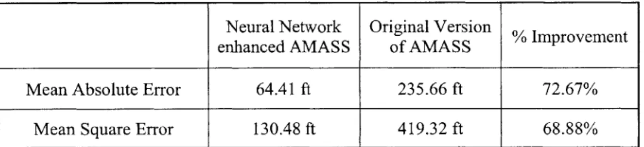
As of January 2003, a neural network had been developed and integrated into AMASS to predict the separation distance between two planes. The neural network used 5 seconds of history and its prediction results are for 10 seconds in the future:

Neural Network _{Original Version} _{/ Improvement} enhanced AMASS of AMASS

Mean Absolute Error 64.41 ft 235.66 ft 72.67%

Mean Square Error 130.48 ft 419.32 ft 68.88%

Table 1. Separation Prediction Neural Network trained with one week of ORD data.

Clearly, the NN enhanced AMASS performed much better than the original version if evaluated with all available data. Unfortunately, the neural network enhanced system did not trigger an alarm in real hazardous situations because it was unable to predict very small separation distances since it had rarely been trained data from hazardous situations. That was the motivating factor to switch to a position prediction neural network. Other weaknesses of the separation neural network surfaced when we investigated different NN

(12)

Weaknesses of the separation distance prediction neural network:

* Alarm Analysis:

When the predicted separation distance between two planes falls below a certain value, AMASS generates an alarm. However, the SDNN network rarely predicts a separation distance in this range. This is because the data used to train the neural network has so few cases of small separation distances. In the real world, aircraft avoid these situations, so they do not show up in the training data. Our research shows that SDNNs trained with more data generates fewer alarms, and it does not sound an alarm on real alarm situations, including ORD 08/21/2001, 02:31:15. Since the motivation of our research is to produce earlier and more accurate alarms, this setback was our basis for switching neural network models.

* Limited length of each training event:

Since the SDNN only monitored planes after AMASS starts monitoring them, it didn't have long periods of separation distance data. AMASS only monitors planes when it gets in the range of the runway. We have approximately 30 seconds for each event. For example, for a 30 second event, using 5 seconds of history means that we only 25 seconds of data can be used in our Output training set (Figure 4). Thus, there isn't much data for the SDNN to learn how to predict separation distance 30 seconds. In addition, we don't have the option of using a longer history input because that would result in even less data to train the future predictions.

5 sec 10 sec 15 sec 20 sec 25 sec 30 sec

---INPUT--j --- OUTPUT---I

Figure 4. Breakdown of 30 seconds of training data.

3.1.2 Position Prediction Neural Network

The team decided that predicting individual airplane positions and then computing SD based on the current position plus predictions would be more beneficial to our goal of

(13)

earlier and more accurate alarms. The advantages and challenges of this design are profiled in this section.

Strengths of the position prediction neural network (PPNN): " Alarm Analysis:

Since the PPNN learns only the flight pattern of a single plane, it is irrelevant that there are so few alarm situations in real life. Later, the incursion distance can be calculate from the aircraft coordinates. The coordinate information will be taken from the position predictions neural network. If the calculated incursion distance falls below a certain level, or if it is negative, an alarm will be generated. Even though negative separation distances don't exist in real life, if one is calculated, it's a warning of an impending collision. " Large number of training events:

The PPNN uses training data from all tracks in the raw FAA logs, not just the planes that AMASS monitors. Since there is data for all planes in the logs, the number of training events is huge. All events are monitored: departure, landing,

taxi, and stopped planes.

" Long individual training events:

The logs monitor each plane for an extended period of time. Some events last up to 10 minutes, providing more data for each event. Since the events are longer, there is more data to teach the PPNN how to predict aircraft position 30 seconds in the future. And since the length of the event is not a factor, we can choose a longer input history size without reducing the available output training data.

Challenges of the position prediction neural network: * Too much data:

Since there is so much data, the training data needs to be filtered before the PPNN can be trained. If the training data is not filtered, the training takes too long (days) to finish. A lot of the longer events are stopped planes, and the neural network might not need 10 minutes of stopped plane data to predict that a stopped plane does not move. There are many ways to filter the training data, and care needs to be taken to filter the data in way such that the neural network learns enough about each aircraft state.

(14)

3.2 Number of Neural Networks

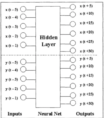
In the SDNN, the inputs were the separation distance between the planes for the past 5 seconds. Thus, there were 5 inputs. In the PPNN, both the x and y coordinates are inputs and outputs of the neural network. We needed to determine whether to have two distinct neural networks, one to calculate the x coordinate output, and one to calculate the y coordinate output. Or whether to use one neural networks with both x and y inputs and both x and y outputs.

2.3.1 Two Neural Networks

Two neural networks are ideal if the x-coordinate prediction is independent from the y-coordinate prediction. However, the system must separate x and y information and make two calls to the neural network module. Using two neural networks ensures a much shorter training time.

For x-coordinate prediction For y-coordinate prediction

x (t +5) y(t +5)

x (t - )+10)

y +1)

x(t3) Hidden x(t+15) y(t- 3) Hidden Y (t +15)

(t-2)Layer x(t+20) y(t-2) Layer

y (t +20)

x (t -1) x (t +25) y (t -1)

y (t +25)

x (t+30) y (t +30)

Inputs Neural Net Outputs Inputs Neural Net Outputs

Figure 5. Two independent neural networks to predict x-position and y-position.

3.2.2 One Combined Neural Network

Using one combined neural network is another option. If the x and y coordinates are not independent, the neural network will adjust the weights in such a way that x inputs have incidence on y estimation. It is practical to use a combined neural network if objects are restricted to move in a known path. Thus it would be useful in predicting train movement, but not airplane movement. In addition, using one combined neural network has the

(15)

x (t -5) x (t -4) x (t -3) 0-x (t -2) O--x (t -1) 0-y (t -5) y (t -4) y (t -3) y (t -2) y (t-1) 0-Inputs x (t +5) x (t +10) X (t +15) Hidden Layer x(t+25) x (t +30) y (t + 5) y (t +10) y (t +15) y (t +20) y (t +25) y (t +30)

Neural Net Outputs

Figure 6. One Neural Network to predict both x and y coordinates.

3.3 Training Algorithm and Neural Network Type

The team had to decide which training algorithm to use to train the new neural networks. We considered both resilient back propagation (trainrp), and the Levenberg-Marquardt algorithm (trainlm). Resilient back propagation is a simple batch mode training algorithm with fast convergence and minimal storage requirements. The Levenberg-Marquardt algorithm is the fastest training algorithm for networks of moderate size. Since our training data set is extremely large, we decided to use resilient back propagation, which was the training algorithm used to train the separation distance neural network. Comparative studies of different types of NN and different training algorithms were performed in order to determine NN type. The group determined that a single layer neural network with 10

hidden nodes was the most appropriate network for our needs [20]. 3.4 Length of History

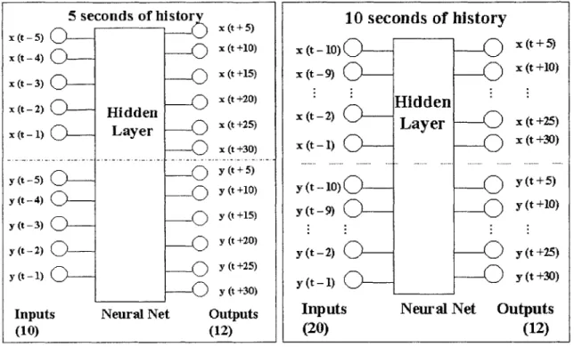
The length of event history affects predictions in the following way. A long history is good for reducing noise while a short history allows for earlier alerts After training the neural network with a longer history, we can look at the weights assigned to the earliest data points. If the weights are very small on the earliest history, it is unnecessary to include

(16)

them. To determine how much history to use, we decided to train PPNN with both 5

seconds of history and 10 seconds of history. The performance of both NNs were analyzed

to determine which network to move ahead with.

5 seconds of histo X (t- - 5 C -1x (t + 5) x (t +10) x (t -4) - _x_(t₊₁₅₎ X~-)( _-3)) - (t yrx x (t +20) -2) Hidden x (t +25) x (t _-- ₁₎ xyert +30) y (t - ) -5 _ _ _ ( y (t + 5) y (t -4) __ Y _{y (t}(t +10)₊₁₅₎ y (t -3) y(t--2) - -y (t +20) y (t - ) y (t +30)

Inputs Neural Net Outputs

(10) (12) 10 seconds of history x (t -10) x (t +5) x(t-9) __ x (t+10) Hidden x (t -2) x ( -2)Layer x (t+2;5) x (t -1) x (t +30) y (t -10) y (t + 5) y (t -9) y (t +10) y (t -2) y (t +25) y (t -1) y (t +30)

Inputs Neural Net Outputs

(20) (12)

Figure 7. Visual comparison of neural networks with 5 seconds and 10 seconds of input.

3.5 Inputs and Outputs

The team considered various types of inputs and outputs to the neural network. We focused on three different options. All three options were carefully analyzed to determine which approach was optimal.

Input (x, y) -> Output (x, y)

Having x and y coordinate inputs and outputs will teach the neural network how planes behave based on the coordinates of the airport. For example, the PPNN might learn that a small section of the airport is a holding place for stopped planes and another path is for taxiing planes. An advantage to this approach is that the neural network is being trained with more information. A disadvantage is that the network might be overtrained. For example, if an airplane lands on a runway in the opposite direction than usual, the PPNN might not be able to predict it's movement if it has only been trained with planes landing in the opposite direction.

(17)

Input (vx, vy, x, y) -; Output (x, y)

This option uses four inputs for each second of history, and the output remains as the x-coordinate and y-coordinate. vx stands for the x-velocity vector, and vy stands for the y-velocity vector. These inputs come from the raw log file, but the team is unsure how these velocities are measured / calculated. Theoretically, the neural network should be able to determine the airplane velocities from the plane position. However, using these numbers as explicit inputs might increase the knowledge of the position prediction neural network. Note that this neural network also depends on

absolute plane position.

Input (dx / dy) 4 Output (dx / dy)

This option uses only calculated velocities to determine future airplane velocities. The input velocities are calculated from absolute coordinates from the airplane history. For example:

dx(t - 3) = distance = x(t -3) - x(t -5)

time 2 seconds

This neural network has only 5 inputs [dx(t - 4) ... dx(t)], and 6 outputs [dx(t + 5)... dx(t + 30)]. The input can be either dx values or dy values depending on the desired output. The advantage of this neural network is that the same neural network can be used to predict dx or dy. Another advantage of this neural network is the absolute orientation and position of the plane are not factored into the predictions, hence avoiding overtraining and enhancing generalization power. If an airplane lands on a runway opposite the customary direction, the PPNN will be able to predict its future positions just as accurately as if the airplane lands in the standard way. If given the initial position of an aircraft, calculating the absolute future position predictions is straightforward using the outputs of this neural network.

(18)

3.6 Training Data Filtering

With such an extensive training dataset, filtering the data is a necessity. In addition, filtering the training dataset is necessary to avoid overtraining. The data can be filtered according to the type of event. The following events are classified by velocity.

Types of events:

Event Threshold (ft/sec)

Stop 0 to 2

Taxi 2 to 80

High Speed 80+

inl. Departure / Landing

Table 2. Classification of aircraft Events.

The three options we are investigating are:

" Case 1: 100% of Stop data, 100% of Taxi data, and 100% of High Speed data. * Case 2: 0% of Stop data, 50% of Taxi data, and 100% of High Speed data * Case 3: Training dataset is evenly balanced with High Speed and Taxi cases.

(Training data: 50% Taxi and 50% High Speed) Note the subtlety in between Case 2 and Case 3.

It is important to give the neural network training examples of different cases which it will predict. However, reducing the training dataset might not adversely affect the PPNN performance if the neural network is not learning from additional examples of the same event. One goal of the filtering is to make the training dataset as small as possible without reducing the performance of the NN. And more importantly, we wish to obtain a good balance of taxi , high speed, and low speed events to teach the network information about

(19)

4. TRAINING AND TESTING THE SYSTEM

This chapter presents the findings of the investigation of the following neural network parameters: history length, neural network inputs, and training data. Section 4.4 presents the optimal neural network resulting from the analysis. Section 4.5 compares the predictive capability of the "optimal" neural network with the current prediction system implemented in AMASS.

4.1 Testing Protocol

The performance of each neural network was tested in two ways.

" Each available training set was broken down into 50% Training Data, 25% Validation Data, and 25% Testing Data. After each neural network was created, it was tested with its Testing Data to evaluate it's performance.

" To objectively compare different neural networks, the neural networks were all tested with the same testing dataset. The data used to test the NNs was extracted from the log file of a different day (ORD 08/20/02) than the training data (ORD 08/21/02). This section presents the results of this objective comparison because it was this comparison that determined which neural network to move forward with. The following neural network was used as the control variable to compare the results of the different networks.

0 5 seconds of input history 0 Input (x, y) -> Output (x, y)

* 0% of Stop / 50% of Taxi / 100% of High Speed Training Data available

The following table shows the performance of the Control neural network when tested with the test dataset. Two error indicators had been computed: the mean absolute error (MAE), and normalized mean square error (MSE). The former is computed as the average of the absolute value of the difference between real position and estimated position. The later is computed as the square root of the average of the squares of the differences. The square root is computed in order to obtain rational units, so that both indicators are expressed in

(20)

Table 3. The AE and MSE for the control NN for each prediction.

NN #1 time in the future Absolute Error Mean Square

(s) Error 5 38.5123 214.4988 X 10 61.1302 214.5783 coordinate 15 118.3901 345.6276 predictions 20 177.801 477.9115 25 238.2453 601.4243 30 326.6187 798.0976 5 17.0812 78.1279 Y 10 52.6802 156.4426 coordinate 15 75.7189 245.5349 predictions 20 120.0383 370.8078 25 166.9513 485.7636 30 222.4006 588.8976 4.2 Length of History

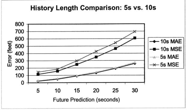
The following table presents the results of NN #2, which takes an input of 10 seconds of past history for both the x and y coordinates. These results will be compared to the control neural network, which takes an input of 5 seconds of past history. Both were tested with the same data set, ORD 8/20/02.

Table 4. Performance of NN with 10 seconds of input data.

(s) Error 5 20.3658 130.9486 X 10 51.9801 171.0901 coordinate 15 104.4055 272.278 predictions 20 150.686 387.0589 25 217.1947 507.6121 30 290.2496 670.8289 5 22.6604 98.2866 Y 10 45.7165 143.7931 coordinate 15 76.3565 223.3593 predictions 20 118.3267 308.7598 25 169.9173 419.2577 30 232.5621 543.7197

(21)

The neural network with 10 seconds of history input performed better than the neural network with 5 seconds of history input. The average difference in absolute error is approximately 10 feet, and the average difference of MSE is 50 feet. These numbers, although small, make an important difference in a safety critical system such as AMASS.

History Length Comparison: 5s vs.

10s

800-700 -600

-+-10sMAE

S500 -4-0s MSE ~'400 -5 A

p300

-5MA

W

20-

5s MSE 100 0 5 10 15 20 25 30

Future Prediction (seconds)

Figure 8. A comparison of the NNs with 5 seconds and 10 seconds of history input.

This experiment shows that future airplane position is dependent on more than the previous 5 seconds of position. Although training a neural network with 10 seconds of past history is more time and computationally intensive, the trade-off in performance is worth the extra time in training.

4.3 Inputs and Outputs

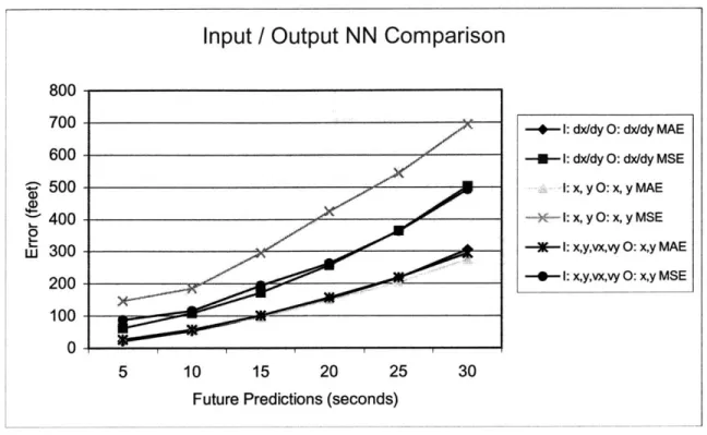
This section presents the results of neural networks with different types of inputs and outputs. Potential inputs include position coordinates, velocity vectors, or coordinates along with velocity vectors. The following table is the performance of a neural network which takes an input of (x, y, vx, vy) for each second of history, and outputs of (x, y) for each prediction interval.

(22)

Table 5. Performance of NN with x, y, vx, and vy as input data.

(s) Error 5 28.6249 94.7369 X 10 60.1002 126.6303 coordinate 15 105.9637 195.2329 predictions 20 165.1381 288.5431 25 234.8033 394.6505 30 314.1055 533.6045 5 25.0464 80.5171 Y 10 54.6794 105.5863 coordinate 15 96.2944 192.5369 predictions 20 146.7566 237.5608 25 203.5444 331.9708 30 275.1589 450.6343

Table 6, below, presents the results of NN #4, which takes an input of either dx or dy, and outputs dx or dy for each prediction interval. Note that this neural network has half the number of inputs as the control neural network (Table 3), and a fourth of the inputs of NN #3 (Table 5).

Table 6. Performance of NN with dx or dy as input and output data.

(s) Error 5 23.0143 69.8669 X 10 56.3569 119.4121 coordinate 15 103.3652 188.5133 predictions 20 161.7185 277.5678 25 231.1155 392.2792 30 310.8419 530.2315 5 20.9678 54.9081 Y 10 50.9114 97.0091 coordinate 15 92.2279 156.4053 predictions 20 143.6874 235.8143 25 203.6226 334.5951 30 271.3923 451.4881

The neural network with an input of dx or dy and an output This neural network is advantageous because it does not need

of dx or dy performed best. two coordinates of input for

(23)

each second of history. The same neural network predicts both the x and y coordinates accurately. Although this neural network outputs velocity values as its predictions, it is easy to convert the velocities into positional predictions. Its position predictions were compared to the output of the test data to determine its performance.

Input

/

Output NN Comparison

800

700 _{_-1:}_{dx/dy 0: dx/dy MAE}

600 -- I1: dx/dy O: dx/dy MSE

500 1: x, y O: x, y MAE

400 - 1: x, y O: x, y MSE

0

L3- -3-00 1: x,y,vx,vy 0: x,y MAE

200 - -I: x,y,vx,vy 0: x,y MSE

100

0

5 10 15 20 25 30

Future Predictions (seconds)

Figure 9. A comparison of the NNs with different inputs and outputs.

Input velocities, compared to input coordinates, result in more accurate predictions because the training set becomes more generalized when coordinate positions are converted into velocities. Thus, there are many more cases to teach the neural network about general flight

patterns. The velocity-input NN learns general airplane movement instead of movement

based on absolute position. A NN which learns movement based on actual position is very

sensitive to its training set selection algorithm and often results in overfitting. Using

coordinate inputs results in poor predictions when an airplane is landing on a runway in an

atypical orientation. For example, if the network is trained with the majority of airplanes

taking off eastward on a given runway, then a plane taking off in the opposite direction

would produce poor predictions using a coordinate based neural network model.

4.4 Training Data

This section presents the performance of neural networks trained with various subsets of

(24)

each other, as well as the control neural network (NN #1), which was trained with 0% Stop, 50% of Taxi, and 100% of High Speed training data available. The following table is the performance of a neural network trained with all of the available training data.

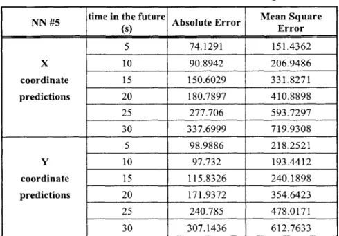
Table 7. Performance of NN trained with all available training data.

NN #5 time in the future Absolute Error Mean Square

(s) Error 5 74.1291 151.4362 X 10 90.8942 206.9486 coordinate 15 150.6029 331.8271 predictions 20 180.7897 410.8898 25 277.706 593.7297 30 337.6999 719.9308 5 98.9886 218.2521 Y 10 97.732 193.4412 coordinate 15 115.8326 240.1898 predictions 20 171.9372 354.6423 25 240.785 478.0171 30 307.1436 612.7633

NN #6, whose results are presented below, was trained with 100% of the available high speed data. The same absolute quantity of Taxi data was also used to train the NN, so the resulting data training set was balanced with 50% High Speed and 50% Taxi data.

(25)

Table 8. Performance of NN trained with a balanced set of training data.

NN #6 time in the future Absolute Error Mean Square

(s) Error 5 39.8228 164.5383 X 10 78.2687 221.8536 coordinate 15 144.9835 349.9594 predictions 20 214.513 506.7347 25 286.3815 635.2542 30 377.6536 801.9031 5 42.493 85.0201 Y 10 98.3929 170.6203 coordinate 15 167.7627 273.7703 predictions 20 266.1394 419.2434 25 354.864 539.8046 30 496.871 711.7728

NN#4, (table 3) trained with 0% of the Stop data, 50% of the Taxi data, and 100% of the high speed data performed the best. It

neural networks.

performed significantly better than the other two

Training Data NN Comparison

800 700 600 -+-Balanced (NN #6) MAE -- Balanced (NN #6) MSE 42 /P-4-- OS,50T,100HS (NN #1) MAE 400 - -- OS,50T,100HS (NN #1) MSE Wi 300 _ -*W-All (NN #5) MAE -*-All (NN #5) MSE 200 ...-100 5 10 15 20 25 30

Future Prediction (seconds)

(26)

The results of this experiment are somewhat surprising. The NN trained with all of the data performed much worse than the winner, which was trained with a subset of all the data. One reason is that the stop data biased the neural network to predict output values too close to the input values. The NN trained with a balanced dataset did not perform well potentially because there was not enough data. Since it performed worst in this experiment, it is best to move forward with the neural network trained with 0% of the Stop data, 50% of the Taxi data, and 100% of the High Speed data.

4.5 Optimal Neural Network

Through the results of the various experiments, an optimal neural network presents itself. The neural network uses dx or dy as its input and output. It takes in 10 seconds of past history as an input. The neural network should be trained with 0% of the Stop data, 50% of the Taxi data, and 100% of the High Speed data.

In conclusion, the new optimal neural network yields accurate position predictions and lends itself easily to predict alarm situations. The advances discovered in this research bring us closer to our goal of earlier and more accurate alarms, which will greatly enhance aircraft safety. Note that the same neural network will be used to predict movement in the x and y independently.

(27)

Optimal Network

dx (t - 10) dx (t - 9) dx (t -6) dx (t +5) dx (t - 7)

Hidden

dx (t -6)

Layer

dx (t +10) dx (t +15) dx (t -5) dx (t + 20) dx (t - 4) dx (t +25) dx (t -3) dx (t +30) dx (t - 2) dx (t - 1)

Inputs

Neural Net

Outputs

(10)

(6)

Trained with 0% of the Stop data, 50% of the Taxi data, and 100% of the High Speed data.

Figure 11. Diagram of the optimal neural network for aircraft position prediction.

4.6 Optimal Neural Network Analysis

The optimal neural network was integrated into the AMASS by modifying the source code

provided by Volpe. Further performance analysis was conducted by running AMASS in

simulation mode to evaluate its performance in the control tower. The performance

comparison conducted so far has only compared the prediction error of the change in X or

Y coordinates. Since the neural network is integrated in to the NN-AMASS at this stage, it

is able to output the predicted separation distance between two airplanes. Thus we can

compare the prediction capabilities of the AMASS prediction model and Neural Network

prediction model. The neural network's performances were evaluated using ORD0821 Log

file, and all the events tested were situations when the AMASS monitors and predicts

airplane separation distances. The test sets were performed on four separate situations; All,

(28)

- All scenarios include all the events except for the Stop-Stop, where both airplanes are in Stop mode. This will provide an overall accuracy of the neural network system compared to the AMASS system.

- HS-HS events include situations where both airplanes are in high-speed mode. The events considered as high speed are Arrival, Landing, Takeoff, and Departure. - LS-LS events are situations where both airplanes are in either Taxi or Stop mode. - HS-LS events are situations where one aircraft is in high-speed mode while the

other is in low speed mode.

The number of events that match each of these categories in the log file ORD821 are in the following table:

Table 9. Distribution of Situations (data points)

Time (sec) Stp-Stp HS-HS HS-LS LS-LS 5 365 203 499 3817 10 254 103 169 2734 15 198 41 48 1972 20 157 4 17 1407 25 130 0 7 987 30 97 0 2 727

As shown in Figure 12, the initial testing shows that the neural network is slightly better at predictions 25 and 30 seconds in the future compared to the AMASS; however, for seconds 5 through 20 in the future, the AMASS seem to be predicting more accurately and consistently. The latter observation leads one to more closely investigate this particular neural network model. Additionally, a look at the distributions of the test situations shows that most situations tested were LS-LS, which are much easier to predict and less likely to trigger an alarm.

(29)

Results Filtered (no Stp-Stp)

NN Prediction AMASS Prediction

MAE MSE MAE MSE

5 172.4 1747.9 71.4 549.8 10 391.1 5163.4 103.4 451.7 15 426 6557.2 138.1 210.5 20 220.3 365 195.4 287.6 25 277.5 409.4 289.2 435.5 30 370.8 546.5 386.8 594 Results HS-HS

MAE MSE MAE MSE

5 770 4137 184 386

10 2482 13673 213 325

15 2700 3115 322 431

20 3149 3312 373 398

25 N/A N/A N/A N/A

30 N/A N/A N/A N/A

Results HS-LS

MAE MSE MAE MSE

5 95 454.7 30.2 162.9 10 405.3 1897.4 40.9 182.2 15 1008.8 4285 22.5 29.2 20 74.7 95.2 23.2 30.2 25 90 96.6 22.6 23.9 30 159 166.6 19.2 19.2 Results LS-LS

MAE MSE MAE MSE

5 38.8639 57.9987 35.2082 56.0249 10 86.0352 128.019 80.3272 123.2421 15 143.5018 209.9712 132.2069 200.9412 20 205.6121 305.1151 194.4219 287.072 25 273.1189 402.6833 289.6508 436.5538 30 367.4307 540.2458 387.3256 594.7503

Figure 12: Results of Position Prediction Neural Networks

For the HS-HS events, future 25 and 30 second prediction comparison could not be

performed because there were no data available. Additionally, some results are misleading,

(30)

Some data was available in predicting future 5 to 20 seconds for the HS-HS and HS-LS situations, however the neural network forecast of the future separation distance is inferior than the AMASS forecast. This is concerning as the most dangerous situations result when both airplanes are at high speed (HS-HS) or at least one is in high speed (HS-LS).

The above comparison illustrates the mediocre accuracy performance provided by this particular neural network system, especially in the events that include high-speed situations. To investigate why the neural network is doing so poorly in the high speed situations, detailed analysis was conducted of an event that took place on Aug 21 02:35:16 when an airplane was landing while another one was on the designated runway.

The coordinates of the landing airplane were not taken uniformly, hence producing large gaps or narrow gaps, as shown in Figure 14. TI is the airplane landing on the runway, and T2 is the airplane taxing on the runway. The non-uniform sampling is a product of the ASR radar system which is less accurate than ASDE.

T1

T2

Figure 13: Simulation of Situation on Aug 21 02:35:16. Note the inaccuracy of the radar sampling rate.

As a consequence, the speed of the airplane appears as non-uniform while in average is 288 ft/s. In Figure 15, the velocity of both aircraft are graphed, and it is clear that the speed of Ti was sampled non-uniformly, while the slow moving target T2 shows a clean signal.

(31)

Current Speed (ft/s) 600.0 500.0 400.0 -+- TI 300.0 -2- T2 200.0 100.0 0.0

Figure 14: Speed of TI and T2 estimated as difference between current position and previous position

Therefore, as shown in Figure 16, the estimation for displacement made by the neural network is not uniform and shows values too large (at 2:35:19) or too small (at 2:35:24).

NN estimations for DeltaX

Figure 15: Estimations of displacement in X direction for T1

The neural network should have taken into account the effect of bad sample spacing to make better estimations, especially because it is using ten samples of the past data. However, it appears that the neural network is not working with the expected level of

40000 35000 30000-25000 -20000 15000 /004zJ 10000 -5000 - -... 0--50% b %b _A t -*- FutureTlDX5 -a-FutureT1DX10 FutureTlDX15 ---x- FutureTDX20 -w- FutureTlDX25 --- FutureTDX30

(32)

accuracy. Figures 17 and 18 show the values of the separation distances for different estimation times: 15 and 20 seconds. Results for 25 and 30 seconds are not shown because most of the real values are not available.

SD 10s 90( 80 70 60 50 40 30

20(

)0.0 30.0 30.0 20.0 30.0 )0.0 -- - - - )0.0 -)0.0 30.0 -+- Real -u--NN Linear

Figure 16: Separation Distance at 10 seconds in Future

SD 20s

30000.0 25000.0 20000.0 15000.0 10000.0-5000.0 0.0 -5000,-b,-,W _b.b-W Z

qf"*O CO, rP CP VCO C ei

-+-Real -u-NN

+Linear

(33)

In order to check if the neural network was correctly implemented in AMASS, graphs were generated to compare the estimation of delta values in X direction with the actual delta values, which are similar to the data used to train the neural network. The graphs in Figure 19 and 20 show very large errors for neural network predictions. In fact, the mean absolute errors were: 531.3 ft (t-5s), 1330.1 ft (t=10s), 2356.1 ft (t=15s), and 3529.4 ft (t=20s), which are not consistent with the accuracy analysis shown previously in this chapter.

Delta values t=1Os

9000 8000 7000 6000 5000 4000 3000 2000 1000 0 -4-Real DX10 -U- FutureT1DX10

Figure 18: Delta X at 10 seconds in Future

Delta values t=20s 25000 20000 15000 -10000 5000 O -5N -+-Real DX20 - FutureT1 DX20

(34)

From the investigation above, it was concluded that re-training of the neural network was necessary. Neural networks are known for their ability to make accurate predictions despite imperfections in the input data. However, our neural network did not robustly handle the flawed input data. Since it could not handle poor sample spacing, a new method of data extraction was investigated and implemented. As explained in Chapter 5, the new extraction method obtains all Landing and Takeoff events in ORD runways, and trains the neural network with this data.

(35)

5. DESIGN PHASE

II:

A

NEW APPROACH

This section discusses the motivation for creating a new approach that involves using two neural networks and a new method for computing separation distance. It also presents the algorithm used for determining the incursion distance between two planes, that is based on trigonometric analysis and yields SD values useful for danger detection.

5.1 ASR and ASDE Neural Networks

Previously, the neural network was trained with coordinate data from ORD log file, with attention given to the balance of stop, high speed, and low speed events. There are two radar systems used at the Chicago O'Hare airport: ASR and ASDE. ASR tracks airplanes in the sky and it is imprecise in its measurements. ASDE tracks airplanes on the airport surface. The new extraction method involves extracting each landing and takeoff event individually. This method is able to handle the switch of the radars as airplane coordinates from both ASDE and ASR radar are appended to make a complete takeoff or landing. Thus, each event is longer, and there will now be enough data to train the neural network to make predictions up to 30 seconds in the future. Note that the previous NN was only trained with two HS-LS events and no HS-HS events for predictions 30 seconds in the future. The obtained coordinates are transformed into neural network input/output pairs (delta input/output) to be used as training sets.

Additionally, the training sets were separated into two sets depending on which radar is tracking the airplane at the time. By dividing the training sets by the radars two neural networks, ASDEnet and ASRnet were trained. The advantage of having two neural network systems is that one neural network (ASRnet) can handle the noise in the input when the airplane is being tracked by ASR radar, while the other neural network (ASDEnet) can be trained for inputs without any noise when the ASDE radar is tracking the airplane. Furthermore, because ASR radar observes airplanes outside of the runways and ASDE radar monitors airplanes on the runways, it can be said that ASRnet predicts the characteristics for high-speed airplanes and ASDEnet predicts the characteristics for low speed airplanes. Furthermore, important work was done to extract landing and departure

(36)

events in every of the six runways at ORD, in order to train the NN for all possible operations [19].

5.3 Incursion Distance Algorithm

The AMASS system sounds an alarm when a negative separation distance is predicted. The first implementation of the neural network into NN-AMASS employed the Euclidean distance formula to obtain the future separation distance between two aircrafts. This distance, Separation Distance, is useful to observe the accuracy of the Neural Network Model, however is disadvantaged in alert triggering as the model is unable to produce negative future distances. The AMASS prediction of the future distance between two airplanes is calculated depending on the positions and the directions two airplanes are travelling. Through this computation method the AMASS is able to attain negative future distances, which will trigger alerts in the safety cell. Therefore, addition of the future distances parameter for alert triggering, called Incursion Distance, is to be included to further enhance the neural network model. This algorithm was primarily designed by Dr. Rafael Palacios.

Using the AMASS code as a reference, the two airplanes will be categorized by the relative position and direction that each airplane is travelling. There are three categories:

- Head-On: Two planes are travelling toward each other. (Figure 21)

- Chase: One plane is travelling similar direction as other airplane. For example a Lander behind Lander. (Figure 22)

- Apart: One plane is travelling opposite direction as other airplane. (Figure 23) Since single-surface events are only considered, all three categories are related to a pair of airplanes moving in the same runway. Therefore we are interested in distances attained along the main runway direction in order to compute current separation distances (CurrentSD) and predicted separation distances (FutureSD).

(37)

Track I - - - Currmet SD TIFutureDY.. _Future_SD TIFurDX ---- T2FutureDxy T]FuureDxy % --- T2FutureDY T2FutureDX Tak2

Figure 20. Head-on event.

T Y - - - OuatSD TIFu ₄ Track I % T2FuaceU T2rardfxY TIFutureDxy - - - Current SD TIFuturDY -- Future SD TIFutureDX _T2FuturcDxy Tracki S ~--- T2FutumDY T2FutureDX Truck 2

Figure 21. Chase Event.

Figure 22. Apart Event. Figure 23. Chase Event, Overtake.

The neural network prediction is used independently for X direction and Y direction, providing values of the predicted distance that the airplane will move in each direction. For example for predictions 20 seconds into the future TlFutureDX20 and TlFutureDY20 are obtained, that represent the distance that target 1 will travel during the next 20 seconds in X and Y direction respectively. The neural network developed is able to simultaneously compute predictions for 5, 10, 15, 20, 25, and 30 seconds into the future. Nevertheless for the following examples, only the variable for 20s in future will be shown.

The estimation of airplanes future positions and the estimation of future separation distance can be obtained using the following equations:

(38)

TlFuture2OX = T1X + TlFutureD20X TlFuture2Y = TlY + TlFutureD20Y T2Future20X = T2X + T2FutureD2OX

T2Future2OY = T2Y + T2FutureD2OY

CurrentSD = V(TlX - T2X 2 +(TlY - T2Y)2

FutureSD20 = (Tl1Future2OX - T2Future2OX) 2 ₊_(TlFuture2OY_- _T2Future2OY)2

Quite often vector TlFuture20xy or vector T2Future2Oxy are not exactly parallel to the runway direction, as shown in previous figures. This is a consequence of small instantaneous changes in bearing, noise in radar signals or error in the estimation of FutureDX or FutureDY. As a consequence CurrentSD and FutureSD get values slightly

larger that the real values.

Another problem is that computing FutureSD by using the basic trigonometric functions of distance always yields positive values. Therefore in a situation like the one depicted in figure 24, where target 2 overtakes target 1, FutureSD computed with the previous equations is a large positive value that will not generate an alarm. In this situation it makes more sense to change the sign of FutureSD and return a negative prediction.

Accordingly, there was a need to define another way to compute predicted separation distance able to produce negative values and able to minimize the impact of noise. That distance is called Incursion Distance.

The best way to minimize the impact of noise in this environment is to identify the runway direction and project every vector over that direction. Moreover, working with projected distances the computation of Incursion Distance is simplified because it is converted just in additions or subtractions.

Figure 25 shows an event similar to the one shown in figure 24 and the projected vectors and distances. Future incursion distance is computed after the values of projected magnitudes (noted with "p").

(39)

owSD

TI

---.-.... S.

-- ~~T2----..

-- - Projected values

Figure 24: Calculation of Incursion Distance in a Chase Event

Using projected magnitudes, computing incursion distance is as simple as the following equation:

IncDist = CurrentSDp + T 1FutureDp - T 2utureDp

According to the angles show in Figure, projected magnitudes are calculated as:

CurrentSDp = CurrentSD -cos((oSD ) T 1FutureDp = T 1FutureDxy -cos(ol )

T 2utureDp = T 2FutureDxy -cos((o2)

The main runway angle (Q) is obtained by rounding the direction (bearing) of the fastest moving airplane, since runway directions are always multiples of 10 degrees. Runway direction should be similar to T2T1 vector. Once Q is known, (01, (o2, and coSD are computed as difference with the basic angles. The basic anbles al, U2, and aSD are easily obtained using atan2 function (in C or Matlab).

al = atan2(T 1FutureD20Y,T 1FutureD20X )

a2 = atan2(T 2FutureD20Y, T 2FutureD20X ) ctSD = atan2(TIY - T2Y, TIX - T2X)

(40)

Figure 26 shows the same category of event in a situation where target 2 is moving at a much higher speed, so that it is able to overtake target 1. In this case incursion distance should be negative, as it is automatically obtained applying the equations.

\ Projected values

Figure 25: Calculation of a Negative Incursion Distance

The only difference with other categories is the way to compute incursion distance. The

equations are:

Head - on : IncDist = CurrentSDp - T 1FutureDp - T 2utureDp Chase : IncDist = CurrentSDp + T IFutureDp - T 2FutureDp Apart : IncDist = CurrentSDp + TIFutureDp + T 2utureDp

Nevertheless it is not necessary to find which particular category is being computed, because being careful with angle definitions, projected vector will automatically become

negative magnitudes. Hence only the first equation was used for implementing calcIncDist function.

(41)

6. PHASE

II FINDINGS

Section 6.1 presents the findings of the dual neural network model. Section 6.2 shows the capability of the neural network model after the incursion distance algorithm was implemented.

6.1 Dual Neural Network Results

After improving the extraction tools and training new neural networks for ASDE and ASR data separately, similar analysis with the 02:35:16 event on August 21 was conducted. The initial result shows that new neural networks are more accurate than previous. Using the current approach, the estimation of delta values is now very accurate, as shown in Figure 27 and 28.