An analytical study on image databases

An Analytical Study on Image Databases

Francine Ming Fang

Submitted to the Department of Electrical Engineering and Computer Science in Partial Fulfillment of the Requirements for the Degrees of

Master of Engineering in Electrical Engineering and Computer Science at the Massachusetts Institute of Technology

June 5, 1997

Copyright 1997 Francine Ming Fang. All rights reserved.

The author hereby grants to M.I.T. permission to reproduce and distribute publicly paper and electronic copies of this thesis

and to grant others the right to do so.

Author

Department of Electical uaterC-nputer Science

- June 5, 1997 Certified by ,, , Accepted by_ . . Dr. Nishikant Sonwalkar Thesis Supervisor Ar4hur C. Smith Chairman, Department Committee on Graduate Theses

An analytical Study on Image Databases By

Francine M. Fang Submitted to the

Department of Electrical Engineering and Computer Science

June 5, 1997

In Partial Fulfillment of the Requirements for the Degree of Master of Engineering in Electrical Engineering and Computer Science

ABSTRACT

Complex information data types such as images are becoming more and more significant in digital communication as modem technology continues to evolve. Because of the increased significance of complex image data types, conventional databases which dealt only with textual and numerical information are no longer adequate. With the help of recent advent of more powerful computers and faster networking capabilities, significant amount of work has began in both the academia and commercial world in searching for better techniques to store and retrieve images in large collections. The goal of this thesis is to understand the current status of these research efforts and learn the technologies in the area of image recognition. Furthermore, it also provides a step-by-step guide for

designing image databases and presents a case study on an existing commercial image database. The thesis is intended to serve as an informational resource for researchers and professionals that are interested in this growing field.

Thesis Supervisor: Nishikant Sonwalkar Title: Director, Hypermedia Teaching Facility

CHAPTER 1 INTRODUCTION ... 5

1.1 TRADITIONAL DBM S'S INADEQUACIES ... ... ... 5

1.2 GENERAL ARCHITECTURE OF AN IMAGE DBMS... ... 6

1.3 QUERIES IN IDBM S ... 7

CHAPTER 2 PATTERN RECOGNITION AND IMAGE ANALYSIS TECHNIQUES ... 9

2.1 SEGM ENTATION ... .... ... 9 2.1.1 Edge Detection... ... 9 2 .1.2 C lustering... ... 13 2.2 SHAPES OF REGIONS ... 17 2.3 T EXTURE ... .... ... ... 18 2.4 M A TC H IN G ... ... ... ... 22 2.5 NEURAL NETWORKS ... 24

CHAPTER 3 IMAGE DATABASE RESEARCH PROJECTS ... 28

3.1 BERKELEY'S DOCUMENT IMAGE DATABASE ... 28

3.1.1 Multivalent Documents ... ... ... 28

3.1.2 System Lim itations ... 30

3.1.3 Proposed Solutions to the Limitations ... 31

3.2 MANCHESTER CONTENT-ADDRESSABLE IMAGE DATABASE (CAID) ... . 35

3.2.1 Architecture ... 35

3.2.2 The D ata ... ... 36

3.2.3 MVQL ... ... 37

3.3 THE ALEXANDRIA DIGITAL LIBRARY PROJECT ... ... 41

3.3.1 Im ag e A nalysis... 42

3.3.2 Similarity Measures and Learning ... ... 43

3.3.3 A Texture Thesaurus For Aerial Photographs... 44

3.4 PHOTO BOO K ... ... 45

3.4.1 Semantic Indexing of Image Content... ... 45

3.4.2 Semantic-preserving image compression... 46

3.4.3 Face Photobook ... 47

3.5 THE CHABOT PROJECT ... ... ... 49

3.5.1 Integration of Data Types... ... 50

3.5.2 POSTGRES... ... 50

3.5.3 Image Retrieval Methods... ... 51

3.5.4 System Analysis... 54

CHAPTER 4 COMMERCIAL IMAGE RETRIEVAL SYSTEMS ... ... 56

4.1 IBM 'S QUERY BY IMAGE CONTENT ... ... ... 56

4.1.1 Image Feature Extraction ... 56

4.1.2 Automatic Query Methods for Query-By-Painting... 57

4.1.3 Object Identification ... 60

4.2 THE VIRAGE IMAGE SEARCH ENGINE... .... .. ... 62

4.2.1 Virage Data types ... ... ... 62

4.2.2 Primitive ... ... ... ... 63

4.2.3 Schema definition... 64

4.3 M ETADATA ... ... ... 68

4.3.1 What is Metadata and Why use it ... ... 68

4.3.2 Issues ... ... ... ... ... ... ... 69

4.3.3 Current Status... ... 69

CHAPTER 5 DESIGNING AN IMAGE DATABASE ... 71

5.1 STORING DIGITAL IMAGES ... ... 72

5.3 Q UERY AND RETRIEVAL ... 75

CHAPTER 6 CASE STUDY: QBIC... 79

6.1 TESTING M ETHODOLOGY ... 79

6.2 TEST RESULTS ... .. ... ... ... 81

6.3 EVALUATION CONCLUSIONS ... ... 83

Chapter 1 Introduction

In the last several years, there has been a significant increase in the amount of digital data being produced such as digital images, video, and sound. This expansion of digital mediums created a need for developing management systems that can handle these types of data. Since traditional databases rely solely on the alphanumerical information for search and retrieval, which is adequate for books, papers or any other type of textual publications, they are inadequate for these new data types. These traditional database systems lack the capability and the flexibility to satisfactorily index and search digital images, videos or sounds by content since it is nearly impossible to describe a painting, movie or song completely by using alphanumeric descriptions alone. Clearly, the creation of a new paradigm for digital information management system is necessary.

In general, a database management system provides several fundamental capabilities for sharing information such as querying, recovery, security, fast access, and data

integrity. These capabilities can be classified into two categories. One concerns with the issues of the physical storage, compression and error correction of the images. The other deals with the management of the images in storage, such as the issue of indexing, searching and retrieval. However, the focus of this thesis is mainly on the indexing, searching and retrieval part of image databases although some issues in data storage are mentioned as well.

1.1

Traditional DBMS's

Inadequacies

Most conventional databases support a number of basic data types, such as integer, floating point numbers and character strings25. To support emerging imaging

applications, a number of database management systems (DBMS) also support arbitrary long binary strings called Binary Large Objects or BLOBs. Although most conventional databases support long fields or BLOBs, most conventional database applications still include only the path or references of images in relational records and stored the actual images on some optical storage system. There are a number of reasons for this strategy. One basic reason is that this strategy meets the requirements for on-line, near-line, and off-line storage of images, including archiving. This means, the data in the databases are of textual or numerical nature only which is clearly insufficient for image databases.

Another function often missing from conventional databases is content retrieval. Typically, querying and retrieval in conventional DBMS are based on their text

descriptive attributes. That is adequate for document databases since searching often involves the content of document texts. With full-text retrieval systems, queries can involve any combination of terms and words contained in text documents. But, this content-retrieval concept cannot be generalized to other data types other than text. For content retrieval on images, more than descriptive phrases are necessary. Ideally, image content retrieval can be done by extracting image features, such as color, shape, texture, and then use these features to guide the queries.

Similarly, in conventional databases, sometime the DBMS allows thumbnail viewing of images. Thumbnails are miniature versions of the full size images, so one screen can display many thumbnails at once. These thumbnails help users organize and manage images visually. Users can quickly scan the displayed images to find the desirable one. However, this is no more than like a screen dump of all images stored on the databases. Users may have to view numerous thumbnails before finding the ones they want. The problem here is that the system does not discriminate enough so it returns very imprecise retrieval results to the users.

1.2 General Architecture of An Image DBMS

There are very few existing products or systems that are exclusively image database management systems. Instead, most image databases are constructed within existing conventional database management systems that already include some features and capabilities that can handle images. Therefore, image database developers typically build an image database on top of a conventional DBMS.

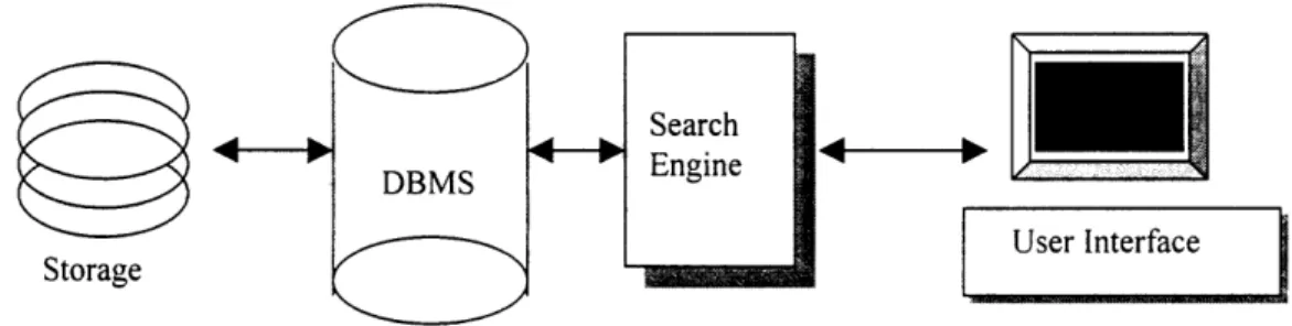
The integration of images into a conventional DBMS can include hierarchical storage modules, content-retrieval engines, graphical editors, and other modules. To meet performance requirements, an image DBMS (IDBMS) may include additional

components such as search engines, spatial data structures, query presentation, and other "extension" modules. Thus the "system" or engine used by an image database typically consists of several objects or modules from different sources. For example, a core DBMS engine, a storage management module, a content-based search engine and a front-end modules such as the user interface. Figure 1 depicts this general architecture.

r Search

D NMS Engine

Storage

User I

_f

1.3 Queries in IDBMS

In conventional "text only" DBMS, the search criteria are on relatively precise attributes such as name, identification number, etc. The user submits a query based on these precise attributes and then obtains the results in a table. The situation is not so clear-cut for image data type queries. Precise attributes such as title and painter are not sufficient for content-based image retrievals. Most of the image attributes need to be extracted from the image itself such as color, texture and shape. Content-based searches can take many forms. For instance, images can be presented as a collection of shapes and then the properties of each shape or object in an image can be parameters in content-retrieval searches. Similarly, the spatial relationship among various objects can be another possible criterion for content retrieval of images. The type of attributes used for retrieval will depends on the intended application. The following are some content retrieval techniques used for image queries25

* Visual queries by example:

The system provides a visual example in an image database so users can find other images similar to it. For instance, the user might pick a fabric and post the query: Show me allfabrics of similar texture in different colors. The query expression thus will involve a GUI environment where the user can pick samples and even compose a query by putting together different objects. An example would be: Give me all still images that have a lamp on the right-hand corner ofa

table just as I have shown here in the sample drawing. In many image database

applications, the sample images in a query are actually obtained from a pick list of a "domain," that is, a set of all possible, typical values for a particular feature or object type. The pick list can be a pick list of colors, textures, shapes, or actual objects, such as facial features in facial-retrieval systems.

* Weights:

In a conventional database query expression, all predicate terms have equal weights. For instances, if the predicate expression is Subject = Correspondence and DateCreated = 10/10/93 then the predicate on Subject and DateCreated must both be satisfied. However, various terms of the predicates can be given different weights by the user. If the query is, say, on "image database", the user can indicate that "image" is more important than "database" in the retrieval

expression. Similarly, this can be applied to image content retrieval where users can indicate, for instance, that the shapes of the objects are more important than the color.

* Similarity Measure:

A search expression in image databases can involve terms like SIMILAR TO where the argument could be a complex image. The image database should

support and contain predefined terms to undergo this kind of complex similarity evaluation. Algorithms must be developed to determine how similar one image is to another. Furthermore, the query results must be returned within an acceptable

amount of response time, and the quality of the images returned in the result must be good. The system must be extendible for development for future functionality. In order to perform content retrieval for images, relevant features in the images must be extracted. Extracting descriptive attribute values or recognizing objects in image databases can be done manually, automatically, or with a hybrid scheme that extracts some of the features automatically while domain experts manually enter additional key features and attributes of the images. Manual indexing is a difficult and arduous task, so it is not ideal for image DBMS. However, a fully automated feature extraction requires the system developers not only to be experts in image feature extractions but also prophets that can foretell what features are ideal for all applications. Therefore, the hybrid scheme is generally preferred. Automatic and manual indexing techniques are often used at different layers of an image database for image recognition and feature-identification components. However, choosing what features to extract and how they can be extracted efficiently is still a challenge for image database developers whether one automate the feature extraction process or not.

Several research and prototype developments of image database applications are currently underway. But before one can fully understand the imaging methodologies that are applied in these image databases, one needs some basic knowledge on pattern

recognition and image analysis techniques. Chapter 2 is devoted to give an overview of the field of pattern recognition and image analysis. In chapter 3, several different image database research projects in academia are then presented followed by chapter 4 that focuses on commercial developments in image databases. Chapter 3 and 4 aim to provide an exposition of imaging database technology, especially on methods for image content retrievals. A guide to designing image databases is then given in chapter 5 while chapter 6 presents the results of an evaluation on a commercial image DBMS.

Chapter 2 Pattern Recognition and Image Analysis Techniques

Prior to being used as inputs to image retrieval programs, images are often modified by going through operations such as segmentation, texture differentiation, and shape recognition so they can become better inputs. These operations extract the images' distinct features to make the image retrieval process easier, faster and more accurate. In this chapter, a brief introduction into several pattern recognition schemes and image analysis technique is given. The areas being explored are segmentation, edge detection, clustering, shape determination, texture differentiation, matching, and neural networks.

2.1

Segmentation

Often, the first step in image analysis is to divide the images into regions that correspond to various objects, each of which is reasonably uniform in some

characteristics in the scene. Afterwards, various features such as size, shape, color, and texture can be measured for these regions and these features then can be used to classify the image. A region can be loosely defined as a collection of adjacent pixels that are

similar in some way, such as brightness, color, or local visual texture. Objects are defined here as non-background regions in the image 6_.

One of the simplest ways to segment an image is to first set thresholds based on pixels' color or brightness that can divide the image into several regions and then

consider each resulting connected region to be a separate object. For example, if

thresholds were set based on pixel's gray level for black-and-white images, the scene can then be divided into light and dark regions. Therefore, one could set n thresholds, which divide the image into n + I categories of gray level, to produce a new image with gray

levels of 0, 1, 2,..., n.

Threshold setting divides the pixels into regions on the basis of their pixels' individual characters, such as gray level, alone. The segmented outcome may be inadequate and unsatisfactory. Another way to segment an image into regions which is not based on single pixel's attributes alone is to look for the discontinuities or edges between the regions and connect them so as to surround, and therefore define, the regions. This is done through a technique called edge detection. Another segmentation technique is called clustering. It is to look for clusters of similar pixels and allow theses groups to expand and merge to fill the regions.

2.1.1 Edge Detection

Edges in pictures are important visual clues for interpreting images. If an image consists of the objects that are displayed on a contrasting background, edges are defined to be the transition between background and objects' 6_{. The total change in intensity from}

detect edges. In the simplest case, first order calculus is used in getting this rate of change. For black-and-white images, the rate of change in gray level with respect to horizontal distance in a continuous image is equal to the partial derivative

g'x = dg(x, y)/dx. This partial derivative can be made finite to become

g'x (x, y) = g(x + 1, y) - g(x, y) Equation 1

Similarly for the rate of change in gray level with respect to the vertical distance becomes

g'y (x, y) = g(x, y + 1) - g(x, y) Equation 2

g'x and g', are called the first differences which represent the change in gray level from one pixel to the next and can be used to emphasize or detect abrupt changes in gray level in the image. Since the edges of objects in a scene often produce such changes, these operators are called edge detectors.

The above edge detectors are quite primitive since it can only detect in horizontal or vertical directions. More sophisticated first difference detectors can operate on a ring of directions as well as on pixels of mixed colors. More sophisticated edge detection is done based on calculating the diagonal differences after performing some rotations. But performing all possible rotations is arduous. For continuous images, the gradient is a vector quantity that incorporates both magnitude and direction. The gradient of the continuous black-and-white image g(x,y) is defined to be the ordered pair of partial derivatives

grad g(x,y) =Vg(x, y) = -g(X, y), g(x, y) Equation 3

yax

ay

The symbol V represents the gradient. The gradient of the continuous image indicates the rate of change in gray level in the images in both the x and y directions. The analogous gradient definition for finite difference operations is

The magnitude M of the gradient is defined by

M = Jg' (x, + g (x,

y)

and the direction D is defined by

D = tan-(g', (x, y)/g'x (x, y)) Equation 6

D is an angle measured counterclockwise from the x-axis. If g' is negative, D lies

between 180 and 360 degrees, otherwise it lies between 0 to 180 degrees. The direction D is the direction of the greatest change in g(x,y), and the magnitude M is the rate at which

g(x,y) increases in that direction.

The edge detectors mentioned earlier are based on first difference methods, so they are most sensitive to rapid changes in the gray or color level from one section to another. But sometime the transition from background to object is quite gradual. In these cases, the edges does not produce a large change in gray or color levels between any two touching sections, but it does produce a rapid change in the rate of change of gray or color level between the regions. To look for a large change of value in the gray level changes in black-and-white images, the second derivative 82g(x,y)/ax2 _{is used, which is}

approximated by taking the first derivative of the first difference image g' ' (x, y) = [g(x + 1, y) - g(x, y)]- [g(x, y) - g(x - 1, y)]

= g(x + 1, y) - 2g(x, y) + g(x - 1, y) Equation 7

Second derivatives are useful only if the gradual gray level changes resemble something like a ramp, a straight line with a constant slope, between the two regions. In real images, it is more likely that the gray level changes will resemble a smooth curve rather than a ramp near the edges of objects. In this case, for two-dimensional images, the edges are often considered to lie at location where the second difference is 0, i.e. where

O2g(x)I3x2 _{= 0 or a2g(x)ady}2 _{= 0. This is called the point of infection.}

2.1.1.1 Laplacian

Just as for the first difference technique, the Laplacian is the counterpart of the gradient for second difference methods. A Laplacian of an image g(x,y) is defined as the sum of its second derivatives,

V2 g(x, y)= a2 + a _{g](x, y) = a2 g(x, y) + a g(x, y)}

2 Equation 8 2ay

The Laplacian operator is well suited for detecting small spots in pictures.

Although some edges show up clearly, the many isolated spots show that random noise in the image is amplified also.

2.1.1.2 Hough transforms

Although second difference methods are better at detecting fading edges, it is not ideal for finding edges in incomplete or noisy pictures. Generalized Hough transforms17 are a set of techniques that can detect incomplete simple objects in images. Hough

transforms detect edges by finding clusters in a parameter space that represents the range of possible variability of the objects to be detected. These transforms are usually used to infer the presence of specific types of lines or curves in noisy images, especially in cases where only fragments of the true line or curve may actually appear in the image. It also applies to faint edges.

The basic idea is to record parameters for each of the lines defined by any pair of points. These parameters should define the line uniquely, regardless of which two particular points on that line originally defined it. For instance, the slope and the y-intercept are frequently used to define straight lines. Thus, as an example, for n points, the edges can be detected by letting the n(n-1)/2 pairs of points define a line and check how many other points fall on or near each of these lines.

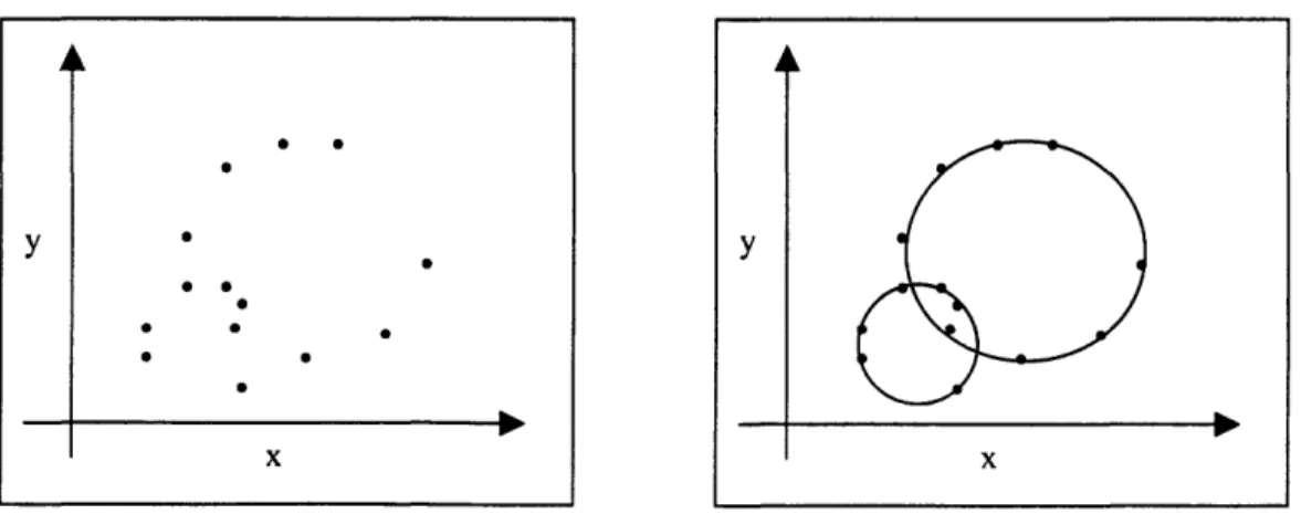
To extend to other family of lines, the steps are the same: first, select features that define the lines; second, make a scatter plot of the results from the feature parameters. The parameter space that is being scatter plotted is called a Hough space. Each pair of points in the image produces one point in the scatter plot. The lines that are actually present in the image produce clusters, dense regions, or peaks in the scatter plot, and are detected by locating these peaks using clustering techniques mentioned in the next section. To illustrate, the detection of existing circles in the image can be done using the

(x,y, r) triplet, where (x,y) are the origin of the circle and r is the radius, and then

determine which value of r that has the most points fallen on it. Figure 2 and figure 3 show this process.

Figure 2. Sampled points in a Hough space (x,y). Figure 3. Two circle detected for the points.

Y * 0 * S I I r\ 10 I I

The methods used to calculate the nearness of other points to a line are least squares and Eigenvector line fitting. Least squares technique minimizes the sum of

vertical squared error of fit, while the Eigenvector method minimizes the sum of squared

distances between the points and the line, measure from each point in a direction

perpendicular to the line.

2.1.2

Clustering

In the previous section they talked about edge detectors, now they are going to introduce another technique often used in image segmentation, clustering. Given a set of feature vectors sampled from some population, they would like to know if the data set consists of a number of relatively distinct subsets. Clustering5 refers to the process of grouping samples so that the samples are similar within each group. These groups are called clusters. The main goal in clustering is to discover the subgroups. In image analysis, clustering is used to find groups of pixels with similar gray levels, colors, or local textures, in order to discover the various regions in the image.

When feature vectors are measured from the samples, finding the clusters is much more than looking for high concentration of data points in a two-dimensional graph. Distinct clusters may exist in a high-dimensional feature space and still not be apparent in any of the projections of the data onto a plane, since the plane is defined only by two of the feature axes. One general way to find candidates for the centers of clusters is to form an n-dimensional histogram of the data, one dimension for each feature, and then find the peaks in the histogram. However, if the number of features is large, the histogram may have to be very coarse to have a significant number of samples in any cell, and the location of the boundaries between these cells are specified arbitrarily in advance, rather than depending on the data.

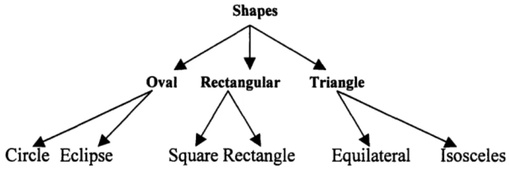
2.1.2.1 Hierarchical Clustering

Hierarchical clustering6 refers to a clustering process that organizes the data into large groups, which contain smaller groups, and so on. A hierarchical clustering helps to manage large feature sets and may be grown as a tree or dendrogram. The finest

grouping is at the bottom of the dendrogram, the coarsest grouping is at the top of the dendrogram. In between, there are various numbers of clusters. Figure 4 shows an example of a dendrogram.

Shapes

Oval Rectangular Triangle

Circle Eclipse Square Rectangle Equilateral Isosceles Figure 4. An example of a dendrogram.

Agglomerative Clustering7 is a type of hierarchical clustering that builds the dendrogram from the bottom up. In this section, the similarity between clusters are measured by the distance between the clusters in their feature space. In other words, each object, such as pixels, is represented as a point in some multi-dimensional feature space. The location of each point is determined by the object's feature attributes. The similarity of the objects is represented as the distance between pairs of samples.

There are four basic algorithms of Agglomerative clustering: single-linkage, complete linkage, average linkage and the Ward's method. The Single-Linkage Algorithm7 is also known as the minimum method or the nearest neighbor method. Similarity is obtained by defining the distance between two clusters to be the smallest distance between two points such that one point is in each cluster. Formally, if Ci and Cj are clusters, the similarity between them SSL is defined as

SSL(C,,C,) = min dist(a,b), Equation 9

aEC ,bEC_,

where dist(a, b) denotes the distance between the samples a and b.

The Complete-Linkage Algorithm" is also called the maximum method or the farthest neighbor method. The similarity between two clusters is determined by

measuring the largest distance between a sample in one cluster and a sample in the other cluster. The most similar clusters are the two clusters that produced the smallest of the maximum differences of all possible pairs of clusters. Formally, if C, and Cj are clusters, the similarity between them SSL is defined as

SSL(C,,C,) = max dist(a,b), Equation 10

aeC_i ,bEC,

where dist(a, b) denotes the distance between the samples a and b.

Both single-linkage and complete linkage clustering algorithms are susceptible to distortion by deviant observations. The Average-Linkage Algorithm" is the

arithmetic averages (UPGMA), and it is one of the most widely used. In this algorithm, similarity is obtained by defining the distance between two clusters to be the average distance between a point in one cluster and a point in the other cluster,

1

SsL(C,,Cj) = Z dist(a,b),

nFnli_j aeCi,bEC

Equation 11

where ni and ni are the number of elements is cluster C, and Cj respectively.

The Ward's Method" is also called the minimum-variance method. It finds two clusters that are most similar to each other by choosing the pair that produces the smallest squared error for the resulting set of clusters. The square error for each cluster is defined as follows. If a cluster contains m samples xl,..., x, and each samples are measured for d features, then x, is the feature vector (fj,...,fjd). The square error for the sample i is

d

S(x,

j=1

Equation 12

where ui is the mean value of featurej for the samples in a cluster.

1-U =

_m

The square error E for the entire cluster is the sum of the squared errors of the samples. m d

E = (xi - ui) = mo"

i=1 j=l

Equation 14

The vector composed of the means of each feature, u = (u,,...,ud), is called the mean

vector or centroid of the cluster. The square error for a set of clusters is defined to be the sum of the square errors for the individual clusters.

2.1.2.2

Partitional Clustering

The Agglomerative clustering creates a series of nested clusters. This is not ideal when what is desired was to create one set of clusters that partitions the data into similar groups. That is called Partitional Clustering8_{. Samples close to one another are}

assumed to be similar and the goal is to group data that are close together. The number of clusters to be constructed can be specified in advance.

Partitional clustering produces divisive dendrograms, or dendrograms formed from top-down, where one initial data set is divided into at least two parts through each iteration of the partitional clustering. Partitional clustering is more efficient than agglomerative clustering since it can divide into more than two at a time, only the top data set is need to start, and doesn't have to complete the dendrogram.

Forgy's Algorithml4 is one of the simplest partitional clustering algorithms. The inputs are the data, a number k indicating the number of clusters to be formed, and k sample points called seeds which are chosen at random or with some knowledge of the scene structure to guide the cluster selection. The seeds form the cluster centroids. There are three steps to the Forgy's algorithm.

1. Initialize the cluster centroids to the seed points.

2. For each new sample, find the closest centroid to it and cluster it together, then recompute the centroids when all samples are assigned a cluster.

3. Stop when no samples change clusters in step2.

Instead of choosing seed points arbitrarily, the Forgy's algorithm can begin with k clusters generated by one of the hierarchical clustering algorithms and use their centroids as initial seed points. One of the limitations of the Forgy's algorithm is that it takes a considerable amount of time to produce stable clusters. However, restrict number of iterations, state a minimum cluster size, and supply new parameters may help in reaching the outcome faster.

The K-means algorithm9 is similar to Forgy's algorithm. The inputs are the same as Forgy's algorithm. However, it recomputes the centroid as soon as a sample joins a cluster, and it only makes two passes through the data set.

1. Begin with k clusters, each containing one of the first k samples. For each remaining n -k

samples, where n is the number of samples in the data set, find the closest centroid to it, and cluster them. After each sample is assigned, recompute the centroid of the altered cluster.

2. Go through the samples the second time, and for each sample, find the centroid nearest it. Put the sample in the cluster identified with this nearest centroid. No recomputing of centroids is required at this step.

Both Forgy's and K-means algorithms minimize the squared error for a fixed number of clusters. They stop when no further reduction occurs. They do not consider all possible clustering however, so they achieve a local minimum squared error only. In addition, they are dependent on the seed points. Different seed points can generate different seed

results, and outcomes may be affected by the ordering of points as well.

Isodata algorithm'0 is an enhancement of the approach mentioned before. Like the previous algorithms, it tries to minimize the square error by assigning samples to the nearest centroid, but it does not deal with a fixed number of clusters. Rather, it deals with

k clusters where k is allowed to range over an interval that includes the number of clusters

clusters if the number of clusters grow too large or if clusters are too close together. It splits a cluster if the number of clusters is too few or if the clusters contain very dissimilar samples. In addition, isodata algorithm does not take a long time to run.

2.2 Shapes of Regions

Once objects are discovered in an image, the next step is to determine what the objects are. The shapes of the object themselves are important to their recognition. A shape has many measures that can define it, and a pure shape measure does not depend on the size of the object. For example, a rectangle that is 8 cm long and 4 cm wide has the same length-to-width ratio, sometimes called the aspect ratio, as a rectangle that is 2 cm long and 1 cm wide. This ratio is dimension-less, and it only depends on the shape of the object, not size.' 8

A ratio of any two lengths of an object could be used as a size-invariant shape measure. One of the important lengths often used is its diameter, which can be defined as the distance between the two pixels in the region that is farthest apart. For a rectangle, its diameter would the length of its diagonal. Likewise, the path length of an object could be defined to be the length of the shortest path that lies entirely within the object, between the pair of object points for which this path is longest. The path length of the letter "S" is the length of the path required to write S. Similarly, the width of an object can be defined to be the width of the narrowest rectangle that encloses the object. Since rectangles only has two parameters or two degrees of freedom that describe them, its length and width, so one measure of shape will suffice to classify its shape. For more complex shapes or objects with higher degrees of freedom, more shape measures will be required to determine their shapes.

Another example of dimension-less measure of shape is the perimeter squared divided by the area of a region P2/A. For circles, this shape measure equals to

P2/A = (2nr 2_)/Iir 2 _{= 4r = 12.57 Equation 15}

for circle of all sizes, and has larger values for all other shapes. For instance, P2_{/A=1 6 for}

all squares and P2/A =20. 78 for all equilateral triangles. But P2/A can approach infinity for

long thin or highly branched objects. As a result, P2_{/A is modified to 4mA/P} 2 _{so it can be} used to produce a shape measure called circularity C, that ranges from 0 to 1.

C = 4zAl/P2 Equation 16

An object in a continuous image is convex if any line segment connecting any two points on the outer boundary of the object lies completely within the object. When an object is not convex, the number of concavities, or their total area divided by the area of the object, can also be used as a shape measure.

Some other interesting shape measures use the concept of symmetry. For example, symmetry classes have been used as features in classifying diatoms, which are single-celled algae33. These microscopic plants are important environmentally because they lie at the bottom of the food chain of a large proportion of all aquatic life. These diatoms show three types of symmetry. Crescent-shaped diatoms have one horizontal line of symmetry. Elliptical diatoms have two lines of symmetry, but if an S-shaped diatom is rotated 180 degrees, it will match its previous position, so it has rotational symmetry.

In breast X-rays, non-cancerous tumors tend to be round while cancerous ones tend to be "spicular" or star-shaped. When a radius is drawn from the center of a rounded object to its edge, it will meet the edge at an angle of about 90 degrees, but for spicular objects, the angle will be considerably smaller, on the avera e. A shape feature based on this concept has been used in the diagnosis of breast cancer .

The medial axis of a region, or the portion of a region left after a technique called thinning, can also serve as a simplified description of the shape and size of an object. Moreover, various parameters based on the branching patterns of the objects can also be used as features for describing shapes. Many other measures of shape are possible. Generally, the nature of the problem determines the types of shape measures that are appropriate to it.

2.3 Texture

The visual perception of texture in an image is created by having regular or random variation in the gray level or color. Various texture features measure the aspects of that variability in different ways. Although human readily recognize a wide variety of textures, they often have difficulty describing the exact features that they use in the

19

recognition process9.

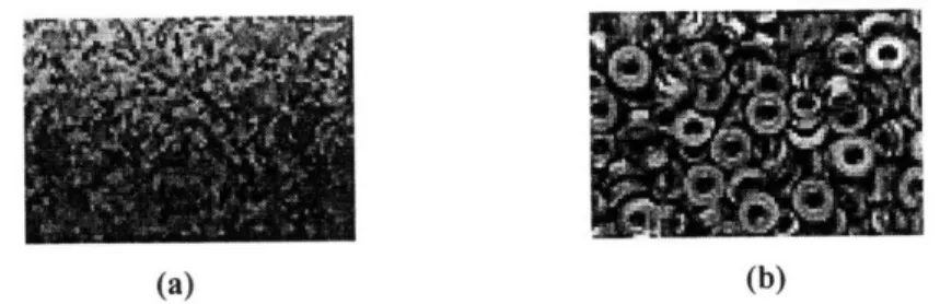
Features based on texture are often useful in automatically distinguishing between objects and in finding boundaries between regions. If a region in an image consisted of many very small sub-regions, each with a rather uniform set of gray level - such as a mixture of salt and pepper -they would say it had a fine texture. But if there regions were large, they would say it had a coarse texture. Thus one measure of texture is based on piece size, which could be taken to the average area of these regions of relatively constant gray level. Figure 5 shows examples or coarse and fine texture samples.

This piece size average can be taken over some predefined region or object or it can be taken in a localized region about any point in the image to measure its texture. Moreover, the average shape measure of these pieces, such as P2_{/A, can be used as a}

Figure 5. (a) an example of fine texture. (b) an example of coarse texture.

Another measure of texture, which still depends on the neighborhood of a pixel, is the variance in gray level in a region centered at that pixel. However, this variance

measure does not require segmentation of the images into regions first. For example, in a

5x5 region, this variance is defined as

1 2 2 2 T,(x, y) = g(x + s, y + t) - g Equation 17

25

25

Similarly, the standard deviation of the gray level in a region can be used as a measure of texture as well.

Run length is another type of measurement that texture can be classified by. First, the number of distinct gray levels in an image should be limited. Limiting the number of gray level can be done by using thresholds for example. Then the image is scanned line by line, and the length in pixels of each run of a certain gray level is

counted. One then can use the average of all these lengths in a region as a measure of the coarseness of its texture. As an example, a three-parameter measure of texture can be based on the average run lengths of dark, medium, and light pixels. Furthermore, parameters of the run-length distributions, such as the variance in the length of the dark run, can be used to detect subtle differences in texture. The relative numbers of light, medium, and dark runs or of various sequences, such as light followed by dark runs, can also be used, depending on how these features vary among the classes to be

discriminated.

2.3.1.1 Co-occurrence Matrices

A slightly more complicated two-dimensional measure of texture is based on gray level co-occurrence matrices20 . The matrices keep track how often each gray level

occurs at a pixel located at a fixed geometric position relative to each other pixel, as a function of its gray level. The (3,17) entry in a matrix for right neighbors, for examples, would show the frequency or probability of finding gray level 17 immediately to the right

of a pixel with gray level 3. Figure shows a 3x3 image and its gray level co-occurrence matrix for right neighbors. The 2 in the matrix indicates that there are two occurrences of

a pixel with gray level 4 immediately to the right of a pixel with gray level 1 in the image.

0012 1000

100

(a) (b)

Figure 6. (a) the original image, the entries indicate the pixels (i,j)'s gray level. (b) the right co-occurrence matrix of the original image, the entries indicate the frequency of a pixel with gray level i being to the right of a pixel with gray level j.

Each entry in a co-occurrence matrix could be used directly as a feature for classifying the texture of the region that produced it. When the co-occurrence matrix entries are used directly, the number of discrete gray levels may need to be reduced. For example, in a 512x512 pixel images with 256 gray levels, the co-occurrence matrix would be a 256 x256 matrix. So the average entry in the matrix will be slightly less than

4, if nearby neighbors are compared. Given this small number, most of the entries probably would be very noisy features for determining the class membership of the region. If the gray levels were divided into fewer ranges, the size of the matrix would be reduced, so there would be larger, less noisy entries in the matrix.

There are many possible co-occurrence matrices. Each different relative position between two pixels to be compared creates a different occurrence matrix. A co-occurrence matrix for top neighbors would probably resemble one for right-side

neighbors for a non-oriented texture such as the pebbles. However, these two-occurrence matrices would probably differ significantly for oriented textures such as bark or straw. Therefore, comparing the resulting co-occurrence matrices for images can also give important clues to its classification.

If the edges between the texture elements are slightly blurred, nearby neighbors may be very similar in gray level, even near the edges of the pieces, In such cases, it is better to base the co-occurrence matrix on more distant neighbors. For example, the matrix entry my could represent the number of times gray levelj was found 5 pixels to the right of the gray level i in the region.

Rather than using gray level co-occurrence matrices directly to measure the textures of image or regions, the matrices can be converted into simpler scalar measures of texture. For example, in an image where the gray level varies gradually, most of the nonzero matrix entries for right neighbors will be near the main diagonal because the gray levels of neighboring pixels will be nearly equal. A way of quantifying the lack of smoothness in an image is to measure the weighted average absolute distance d of the matrix entries from the diagonal of the matrix:

d =1 -I _i -

jmU,

M,

where

M = E mY Equation 20

If all the nonzero matrix entries were on the diagonal,

li-jl

The total length of all the edges in a region can also be used as a measure of the fineness or complexity of a texture. A good source of texture features is the data.

Examination of typical scenes to be segmented or objects to be classified will show how they vary in their textures, and features should be chosen that quantify this observed variation.

2.3.1.2 Fourier Transform

There are occasions where global information may be desirable in classify textures such as how often certain features repeat themselves. In these cases, they can consider the images to be waveforms, and they are looking for repetitive elements in the waveforms. The same transform methods that were used for processing waveforms can then be generalized to analyze the variation of the gray levels in two-dimensional images. Although these transform methods, such as the discrete Fourier transform21_{, is more}

useful for analyzing sound waves that it is for images because sound waves tend to be more periodic than most images. In this type of analysis, rapid changes in an image generally correspond to the high frequencies in the waveform while the gradual changes correspond to the low frequencies in the waveform.

Consider an NxM image for which a typical gray level is g(x,y). The definitions of the two-dimensional cosine and sine transforms are

N-1 M-1

H, (f, fy) = 1 E g(x, y)cos(2nfxx/N + 2nf y/M)

x=O y=O

N-1 M-1

H

(fxI fy) =

g(x, y) sin(2nfx/N + 2rnfy/M)

Equation 21

x=O y=O

The amplitude spectrum is computed as

A(f, fy) =

VH,(fx,

fy) +

Equation 22

2.4 Matching

Often in image recognition systems, there is a large collection of base objects, objects that unknown objects can be compared to so they can be identified. The comparison of the known base object models with an unknown is called matching1

Matching techniques are often used in the analysis of aerial pictures. Matching is useful in comparing two aerial images of the same area that are taken at different periods of time. In general, one of the images must be shifted, rotated, and scaled so that

corresponding objects in the two images coincide. The required combination of transformations required to match one image with another can be considered to be a linear transformation of the coordinate system, from ( x', y') to (x, y), defined by

x = ax'+by'+c₁

y = a2x'+by'+c2 Equation 23

The coefficients of the transformation can possibly be found from the heights, positions, and headings of the airplane that were taking the pictures, or by imaging a standard test object in both pictures as the orientation point. Trial and error may also be required to find the best-matching position. A parameter such as the sums of the average absolute difference in gray levels between corresponding pixels in the two images can be calculated for various transformations, and the transformations that gives the best match can be chosen in this way.

2.4.1.1 Graph Matching

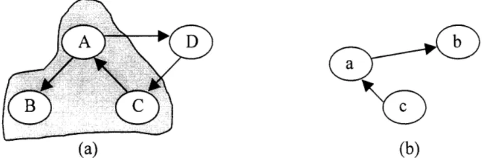
Graphs are a very powerful data structure for many tasks in image analysis. They are often used for the representation of structured objects. In image recognition, known objects are often represented by means of graphs and stored in a database. If both known and unknown objects are represented by graphs, the detection or recognition problem then becomes a graph matching3 problem.

Generally, the term graph matching refers to the process of comparing two or more graphs with each other. There are several classes of graph matching. In the graph

isomorphism problem, they want to determine if two given graphs are isomorphic to each other. Two graphs are isomorphic to each other if they are structurally identical. In the subgraph isomorphism problem, they are given two graphs gl and g2, and want to find out if g2 contains a subgraph that is isomorphic to gl. More generally, bidirectional subgraph isomorphism between g, and g2 means the existence of subgraph g', and g'2

of gl and g2, respectively, such that g', and g'2 are isomorphic to each other. Finally, in

error-tolerant graph matching, they want to find a graph that is the most similar to the one compared to.

(a) (b)

Figure 7: the subgraph enclosed by the gray area in graph (a) is isomorphic to the graph (b) where node A corresponds to a, node B to b, and node C to c.

There are many variation to the algorithms that perform these graph matching problems, the best ones are based on tree searching with backtracking. Each path from the root to the leaves in the tree represents a possible matching of the graphs or

subgraphs. The best match is chosen by iteratively minimizing an objective function that represents the distance of the current solution to the correct solution. Graph matching problems are shown to be NP complete problems. This means that all available methods have exponential time complexity. Therefore, although graph matching can return a satisfactory comparison result, it usually takes too long or too much memory space. Most graph matching algorithms utilize some lookahead techniques and prune dead ends in the search tree as early as possible.

2.5 Neural Networks

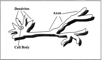
The reason that human brain can perform so efficiently is that it uses parallel computation effectively. Thousands or even millions of nerve cells called neurons are organized to work simultaneously on the same problem. A neuron consists of a cell body, dendrites which receive input signals, and axons which send output signals. Dendrites receive inputs from sensory organs such as the eyes or ears and from axons of other neurons. Axons send output to organs such as muscles and to dendrites of other neurons

Figure 8: A diagram of a biological neuron.

Tens of billions of neurons are present in the human brain. A neuron typically receives input from several thousand dendrites and sends output through several hundred axonal branches. Because of the large number of connections between neurons and the redundant connections between them, the performance of the brain is relatively robust and is not significantly affected by the many neurons that die every day. The brain shows remarkable rehabilitation by adaptation of the remaining neurons when damages occur.

The neurons in many regions of biological brain are organized into layers. A neuron in a layer usually receives its inputs from neurons in an adjacent layer.

Furthermore, those inputs are usually from neurons in a relatively small region and the interconnection pattern is similar for each location. Connections between layers are mostly in one direction, moving from low-level processing to higher coordination and reasoning.

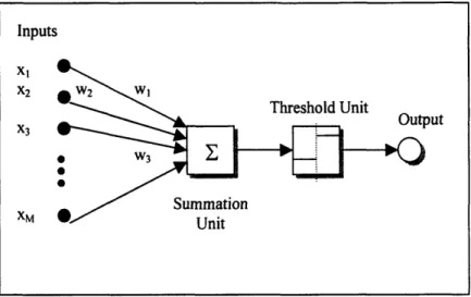
An early attempt to form an abstract mathematical model of a neuron was by McCulloch and Pitts in 1943. Their model receives a finite number of inputs xl..., xW. It

M

then computes the weighted sum, S = wix, using the weights wi, ... w,, which are the

weights for each of the xi inputs respectively. After obtaining S, it then outputs 0 or 1 depending on whether the weighted sum is less than or greater than a given threshold

value T. Summations is indicated by a sigma and thresholding is shown by a small graph of the function. The combination of summation and thresholding is called a node in an artificial neural network. Node inputs with positive weights are called excitory and node inputs with negative weights are called inhibitory. Figure 9 shows an artificial neuron representation.

Figure 9. An artificial representation of the neuron. "

The action of the model neuron is output 1 if

wxI + wX2 + ... + wmxM > T Equation 24

and 0 otherwise. For convenience in describing the learning algorithms presented later in this section, they rewrite Equation 24 as the sum

D = -T+ wix1 + w2 2+ ... + WMXM Equation 25

In which output is 1 if D > 0 and output is 0 if D _< 0.

A difficult aspect of using a neural net is training, that is finding weights that will solve problems with acceptable performance. In section, they will discuss the back-propagation algorithm for training weights, and later in the section, they will discuss Hopfield's network. Once the weights have been correctly trained, using the net to classify samples is straightforward.

Inputs

put

2.5.1.1 Back-Propagation

The back-propagation procedure36 _{is a relative efficient way to train the neural}

nets. It computes how much performance improves with individual weight changes. The procedure is called the back-propagation procedure because it computes changes to the weights in the final layer first, reuses much of the same computation to compute changes to the weights in the penultimate layer, and ultimately goes back to the initial layer.

The overall idea behind back-propagation is to make a large change to a particular weight, w, if the change leads to a large reduction in the errors observed at the output nodes. For each sample input combination, you consider each outputs' desired value, d,

its actual value, o, and the influence of a particular weight, w, on the error, d - o .A big change to w makes sense if that change can reduce a large output error and if the size of that reduction is substantial. On the other hand, if a change to w does not reduce any large output error substantially, little should be done to that weight.

Note that any changes to the weight of particular node will also affect and possibly change the weights of nodes that are close to it. This is the propagation effect. This is the reason why this procedure computes the desirable weights of the last layer of nodes first and then works backward to the first layer.

2.5.1.2 Hopfield Nets

A distinctive feature of biological brain is their ability to recognize a pattern give only an imperfect representation of it. A person can recognize a friend that he or she has not seen for years given only a poor quality photograph of that person; the memory of that friend can then evoke other related memories. This process is an example of associative memory. A memory or pattern is accessed by associating it with another pattern, which may be imperfectly formed. By contrast, ordinary computer memory is retrieved by precisely specifying the location or address where the information is stored. A Hopfield2' net is a simple example of an associative memory. A pattern consists of an n-bit sequence of 1s and -ls.

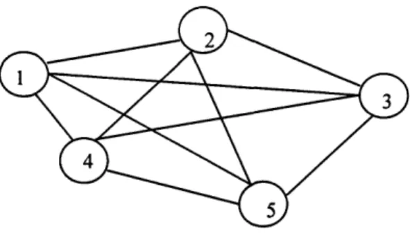
While the nets discussed in the previous sections are strictly feed-forward (a node always provides input to another node in the next higher layer), a Hopfield net every node is connected to every other node in the network.(See figure 10.) Each connection has an associated weight. Signals can flow in either direction on these connections, and the same weight is used in both directions. Assigning weights to a Hopfield net is interpreted as storing a set of example patterns. After the storage step, whenever a pattern is presented to the net, the net is suppose to output the stored pattern that is most similar to the input pattern.

Figure 10. A Hopfield graph.

In the classification step, the n nodes of a Hopfield net are initialized to the n feature values of a pattern. Each node represents one of the n features. Each node concurrently computes a weighted sum of the values of all the other nodes. It then changes its own value to +1 if the weighted sum is non-negative or to -1 if the weighted sum is negative. When the net ceases to change after a certain point in the iteration process, the net is said to have reached a stable state. In practice, a stable state will be detected if the state of the net does not change for some fixed time period depending on the speed and size of the net. If the net functions correctly, it converges to the stored pattern that is closest to the presented pattern, where the distance between two bit strings x and y is the number of positions in which the corresponding bits of x and y disagree. In practice, however, if the net capacity is not large enough, the net may not produce the stored pattern closest to the input pattern. Experimental results show that a Hopfield net can usually store approximately 0. 15n patterns, where n is the number of nodes in the net. If too many patterns are stored, the net will not function correctly.

Although using a nearest neighbor algorithm to compute the stored pattern closest to the input pattern might be more straightforward, one attractive feature of the Hopfield net is that all the nodes in the net can operate asynchronously in parallel. Suppose that the nodes asynchronously compute the weighted sum of the other nodes and that they re-compute and change their states at completely random times, such that this occurs on the average once every time unit.

Hopfield net have been used to recognize characters in binary images. Although a major advantage of Hopfield nets is that all the nodes can operate asynchronously, a major disadvantage is that every node might be connected to every other node. This can become unwieldly in a net with a large number of nodes.

There are numerous uses of neural nets. Neural net is currently one of the most effective way researchers have found to simulate intelligence in computers. Neural nets are used in areas of optical character recognition, face recognition, machine vision and of course pattern recognition.

Chapter 3 Image Database Research Projects

3.1 Berkeley's Document Image Database

One of the many possible applications of image databases is to handle electronic publications. When paper documents are converted into scanned digitized images, these

documents can be easily translated into text by optical character recognition (OCR) products. The UC Berkeley Environmental Digital Library Project26 _{is one example of}

such systems. It is one of the six university-led projects that were initiated in the fall of 1994 as part of a four-year digital library initiative sponsored by the NSF, NASA and ARPA. The Berkeley collection currently contains about 30,000 pages of scanned

documents. The documents consist of environmental impact reports, county general plans and snow survey reports.

The documents enter the database system through a production scanning, image processing and Optical Character Recognition operation that is currently based on commercial technology. The scanner produces 600 ppi TIFF files at 15-20 pages/minute. The OCR software is an "omni-document" system (Xerox ScanWorX) whose capabilities are typical of those found in other state-of-the-art products and research systems. A metadata record is manually created for each document, containing a typical set of fields such as title, author, publication year, document type, etc. These records are entered into a relational database and fielded search is provided via a form-based interface. In

addition, the ASCII files produced by OCR are used for full-text retrieval (currently using FreeWAIS 5.0).

The collection can be accessed through the World-Wide-Web at

http://elib.cs.berkeley. edu/. Most of the testbed services are available using standard

HTML browser, only a few advanced capabilities require a Java-compliant browser. The basic display representation for a retrieved document is the scanned page image,

specifically a 75 ppi, 4 bit/pixel GIF file. A simple page-based viewer provides standard

next-page / previous-page / goto-page navigation. For rapid browsing, the recognized text of a document can be viewed as a continuous ASCII scroll with embedded links to the page images, a format called hyper-OCR. It also has an advanced viewer that is based on the multivalent document (MVD) paradigm. The MVD paradigm will be presented later. One of the features on the MVD browser is the use of word location information

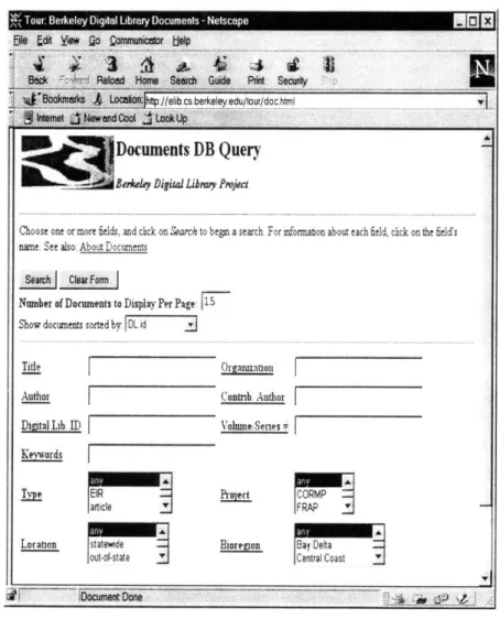
provided by ScanWorX. It highlights search terms in the scanned pages and provides text "select-and-paste" from the page image to a text input buffer. Figure 11 shows the web interface for the system.

3.1.1

Multivalent

Documents

Multivalent Documents35 _{is a new paradigm for the organization of complex digital}

document content and functionality. The multivalent view of a document contrasts with monolithic data formats that attempt to encompass all possible content types of the

document in a single, complicated specification, and provide for interaction with them with concomitant complicated editors, often of limited extensibility. This means that, especially for specialized documents, the monolithic type of systems can be

overwhelming and lacking simultaneously to the users.

†

-Edle die o o uicow

Back U~DWRla Hme Serb Guide

o c hp /lib c berkeley ed/tour/doc html I b~m o ed ni iWt Look Up

Documents DB Query

Beeley Digital Libry Prject

Choose one or more fields, and click on Search to begin a search For mformation about each field, click on the field's

name. See also: About Documents

iPrin Secuy~

-Number of Documents to Display Per Page:

i

Show documents sorted by FDL id

Title Author DigitalLib ID, Keywords Type EIR larticle .J Location [statede out-ofstate o Orgaization Contnb Author VolumeSenes

Bioregon Bay Delta

Central Coast

IaocumentDone

Figure 11. The Berkeley Document Image Database's Web Interface

In contrast, the multivalent approach "slices' a document into layers of more uniform content and then have different operators for each layer acting on the respective uniform content. Additional layers can be implemented when desired. Functionality to these layers is provided by relatively lightweight, dynamically-loaded program-objects, called "behaviors" that manipulate the content. Behaviors of one layer can communicate with other layers and behaviors. Figure 12 shows an example of one document's semantic layers and the behaviors.

In conceiving of documents as interacting layers of content and functional behaviors that unite to present a single conceptual document, this paradigm is able to introduce new capabilities and benefits. For example, by representing a document as

":"::'i:""[I] '" : " """'o";"·": :I : • " ': I'

il--·-iilili- __I_- ii-~·-;·irx~- ^. _.~.~~^.^I;^:;I~..~...~..;.. r-·::;:r::: : :::: : :1:;_:::

multiple components, people besides the original document's author can add additional content and behaviors at later time. This also allows new techniques in dealing with documents to be added whenever it is wanted. This paradigm is flexible since these additions can be made locally, without special cooperation of the server of the base document. In addition, by keeping the pieces of content simple, the behaviors that manipulate them are relatively straightforward to define. The components are also more easily reusable.

-- 0

User outline area Word location Paragraph location

Semantic layers Behaviors

Figure 12. At left, the content of a scanned document conceptualized as semantic layers of

information. At right, the programmatic or behavior implementation of a layer. 35

3.1.2

System Limitations

The document recognition capabilities of the Berkeley system appear capable of supporting a quite useful level of document indexing and retrieval services. However, there are two important areas that the Berkeley researchers have faced challenges in attempting to develop more advanced services.

First, character recognition accuracy for their system tends to vary significantly across documents and is sometimes unacceptably low. The current OCR technology's accuracy is usually adequate on passages of plain English text. However, the error rate is frequently too high to use the text in new documents (e.g. via the MVD select-and-paste mechanism) without thorough proofreading. Furthermore, many of the testbed documents contain tables of statistical data that the users want to import into spreadsheets, new reports, etc. This material must be transcribed essentially without error in order to be useful. Thus, the error rate is often much too high for ideal operation.

r •