HAL Id: hal-00260435
https://hal.archives-ouvertes.fr/hal-00260435
Preprint submitted on 4 Mar 2008HAL is a multi-disciplinary open access archive for the deposit and dissemination of sci-entific research documents, whether they are pub-lished or not. The documents may come from teaching and research institutions in France or abroad, or from public or private research centers.
L’archive ouverte pluridisciplinaire HAL, est destinée au dépôt et à la diffusion de documents scientifiques de niveau recherche, publiés ou non, émanant des établissements d’enseignement et de recherche français ou étrangers, des laboratoires publics ou privés.
POROUS MEDIA: APPLICATION TO BUILDING
STONES.
Emmanuel Le Trong, Olivier Rozenbaum, Jean-Louis Rouet, Ary Bruand
To cite this version:
Emmanuel Le Trong, Olivier Rozenbaum, Jean-Louis Rouet, Ary Bruand. A METHODOLOGY TO SEGMENT X-RAY TOMOGRAPHIC IMAGES OF MULTIPHASE POROUS MEDIA: APPLICA-TION TO BUILDING STONES.. 2008. �hal-00260435�
TOMOGRAPHIC IMAGES OF MULTIPHASE
POROUS MEDIA: APPLICATION TO
BUILDING STONES.
by
Emmanuel Le Trong, Olivier Rozenbaum, Jean-Louis Rouet
and Ary Bruand
Institut des Sciences de la Terre d’Orl´eans, UMR 6113 - CNRS/Universit´e
d’Orl´eans, 1a, rue de la F´erollerie, 45071 ORL ´
EANS Cedex 2
E-mail: manu@mixtion.org
Abbreviated running title: Segmentation of micro-tomographic images
Abbreviated authors:
Le Trong E et al.
Key words:
alternate sequential filter, building stone
mathematical morphology,
segmentation,
watershed, X-ray tomography
ABSTRACT
An image analysis technique based on mathematical morphology tools dedicated to the segmentation of X-ray tomographic images of porous media is presented in this arti-cle. It consists in an efficient denoising using alternate sequential filters and a watershed operation using an original starting marker. The image is transformed into a mosaic that is straightforward to segment. An application to building stones of heritage monuments illustrates the potentialities of this technique.
INTRODUCTION
Exposed to their climatic environment, the building stones of heritage monuments are often altered and eventually destroyed. This phenomenon called weathering is visible throughout the world and many studies in this field, led with architects and restorers, aimed at finding processes to slowing down, controling or ultimately avoiding this de-cay (Amoroso and Fassina, 1983; Tiano et al., 2006; Torraca, 1976). A way to achieve such a goal is to understand the weathering mechanisms of building stones, i.e. to relate the microscopic mechanisms occurring at the pore scale (dissolution of minerals, transport, precipitation, etc.) to their consequences at the macro-scale (desquamation, powdering, etc.) (Amoroso and Fassina, 1983; Camuffo, 1995; Trk, 2002). Some studies comparing weathered stones with unweathered stones were performed. The chemical and mineralogical composition, as well as the porosity were analysed (Rozenbaum et al., 2007; Maravelaki-Kalaitzaki et al., 2002; Galan et al., 1999). The main processes of weathering were thus qualitatively inferred from the differences identified. However, a more quantitative understanding of these weathering mechanisms (fluid flow, dissolution, mass transport, crystallization) and their consequences is to simulate them via a com-puterized model. This requires in turn a quantitative, realistic description of the three dimensional structure of the porous medium (Dullien, 1992; Adler, 1992; Anguy et al., 2001). Such a goal can be achieved with a promising and increasingly developping tech-nique: X-ray tomography. Tomography designates the generic technique of constructing a 3-d image of a sample given several projections recorded at various angles (Kak and Slaney, 2001). It is a non-invasive method that enables the visualization of the inner structure of the stone. By using a X-ray light source, the resulting 3-d grey level image is a map of the X-ray absorption coefficient of the various phases constituting the sample. The synchrotron X-ray radiation source, compared to the more conventional X-ray tube, brings several crucial advantages such as beam stability, high flux, monochromaticity, high coherence and parallelism of the beam, that lead to high quality and high resolution images. It is a key technology enabling to measure accurately the inner structure of a
material.
However the segmentation of a raw tomographic image is seldom a trivial process, highly dependent on the starting image and the objects to extract from it. Segmentation is the process of partitioning billions of grey-level voxels of a 3-d image into distinct objects or phases. The goal, in the context of building stones, will be to separate the void phase (here actually filled with resin) from some distinct solid phases (two for the stone under study). Most of the segmentation complexity is related to the presence of noise (voxels with the same grey value can actually belong to two different phases) and blur (the borders between the phases are not well defined). Moreover, because the images are big and three-dimensional, the analysis cannot be done by hand (e.g. by marking the objects of interests) and must be as automated as possible. The main techniques found in the literature are:
– Thresholding the grey levels histogram, with (Kaestner et al., 2006) or without (Ap-poloni et al., 2007) a former filtering, with automatically (Sezgin and Sankur, 2004) or manually (Appoloni et al., 2007) determined thresholds. The thresholded images sometimes have to undergo a binary post-treatment to adjust the results of these approaches. It is most of the time a reconstruction of the connected components of interest (du Roscoat et al., 2005; Lambert et al., 2005; Kaestner et al., 2006; Erdogan et al., 2006).
– Active contours on the image considered as a level set (Ramlau and Ring, 2007; Chung and kin Ho, 2000; Maksimovic et al., 2000; Qatarneh et al., 2001). These techniques are mostly used in medical applications and usually require a marking of the objects to be extracted.
– Watershed-based techniques (Videla et al., 2007; Malcolm et al., 2007; Benouali et al., 2005; Carminati et al., 2006).
The segmentation step of the images of the stone under study, which falls in the third above category, is the subject of this contribution. It will be shown that the characteristics of these images lead toward a sophisticated de-noising technique based on a watershed mosaic-like operator (Beucher, 1990), using a carefully and automatically chosen marker. Following this introduction, section 2 presents the stone used in this study that serves as model stone, the sample preparation, and the images obtained on the ID-19 tomographic beamline at the ESRF (Grenoble, France). Section 3 details the image analysis procedure, based on mathematical morphology tools, used to segment the images. It also presents some preliminary results. Section 4 concludes this contribution.
X-RAY MICRO-TOMOGRAPHY OF TUFFEAU
SAM-PLE
←insert Fig. 1←insert Fig. 2
Most heritage monuments (chˆateaux, churches, cathedrals or houses) constituting the cultural heritage of the Loire valley, that is registered to the World Heritage list of the UNESCO (UNESCO, ????), are made with tuffeau, a highly porous limestone (porosity
≈ 45%) originating from this valley. Previous studies (Dessandier, 1995; Brunet-Imbault,
1999; Rozenbaum et al., 2007) showed that minarals are essentially sparitic (large grains) or micritic (small grains) calcite (≈50%), silica (≈45%) in the form of opal
cristobalite-tridymite spheres and quartz crystals, and some secondary minerals such as clays and micas in much smaller proportion (a few %). The scanning electron microscopic (SEM) image in figure 1 illustrates the structural complexity of the main phases of tuffeau.
X-ray tomography (Kak and Slaney, 2001) is a choice technology to extract the structure of samples of various porous materials: rocks (Lindquist and Venkatarangan, 1999; Sheppard et al., 2004; Appoloni et al., 2007; Betson et al., 2004; 2005; Videla et al., 2007), cements and ceramics (Erdogan et al., 2006; Maire et al., 2007), soils (Gryze et al., 2006; Carminati et al., 2006) and others (Jones et al., 2004; Mendoza et al., 2007; du Roscoat et al., 2005; Prodanovi´c et al., 2005). The objective is usually to characterize
the medium or to simulate some physical processes in a realistic geometry. Our ultimate objective pertain to both categories. The typical sizes of the structural components of tuffeau relevant to fluid flow, like micritic calcite grains (a few m in size) and opal spheres (10 to 20 m in size), suggest the use of a high resolution tomograph, which leads toward synchrotron radiation facilities. However the smallest structures such as those related to the opal spheres roughness or phyllosilicates will not be accessible as their size is far below the best resolution any X-ray tomographic facility can achieve nowadays.
The microtomographic images presented in this study were collected at the ID-19 beamline of the ESRF (European Synchrotron Radiation Facility, Grenoble, France) (Salvo et al., 2003; Baruchel et al., 2006) at the smallest possible pixel size: 0.28 m. The energy used was 14.7 keV and 1500 successive rotations of the sample corresponding to 1500 angular positions ranging between 0 and 180 were acquired by the FReLoN camera with 2048× 2048 pixels image size. In order to stay in the field of view of the detector and
avoid supplementary artifacts, the samples have to measure less than 700 m in diameter. They were prepared as cylindrical cores of that diameter and were mounted on a vertical rotator on a goniometric cradle. Preparation of a tuffeau sample of such a size requires particular care. Samples were impregnated with a resin in order to make a 700 m thin section. This latter was cut into matches of square section and finally trimmed to obtain quasi-cylinders of diameter ≈ 700m. Imaging time was approximately 45 minutes and
the 2048 horizontal slices (0.28 m thick) were reconstructed from the projections with a dedicated filtered back-projection algorithm. The outputs of the tomographic process are then images of 2048× 2048 × 2048 voxels with 256 level grey level values (one
uncompressed image is then 8 GB in size). The grey level value of a voxel is linked to the X-ray absorption of the sample at the voxel position (Baruchel et al., 2000). Thus, the pores appear in dark grey, the silica compounds in medium grey and the calcite compounds in light grey in figure 2. The different phases are easily distinguishible to the naked-eye and it is clear that the sample size is sufficient to catch the wide scale range of the different structural components. Calcite is present in the form of large irregular grains (sparitic calcite) or small grains that look like crumble (micritic calcite). Silica has
the form of large quartz crystals or small spheres of opal.
Hence it is not possible to rely on some shape or size criteria to identify the phases and only the grey level is relevant. The problem is although looking smooth naked eye, the images are in fact noisy as shown in figure 3-(a). This noise randomly affects the grey value of the voxels, preventing to label them solely from their grey values. In other words a mere threshold on such an image would yield a blatantly incorrect result. This noise effect is also visible on the image histogram: it is smoothed (see the histogram of the original image in figure 4). Theoretically, a perfect image of tuffeau (without noise) would contain only voxels with three precise grey values, one for each phase (resin, silica, calcite). Its histogram would then consist of only three peaks at these values. On the other hand, the voxel values of a noisy (i.e. real) image are randomly disrupted, given then intermediate values. The histogram is then smoothed and the peaks corresponding to the three phases are difficult to separate. Since it can only rely on the grey level to distinguish the phases, the segmentation technique will actually consist in an efficient denoising of the images: enough noise must be removed to identify the phases, without blurring wich leads to loosing the small structures of the images (e.g. micritic calcite). Some basic smoothing filters (e.g. a mean filter) have been found unable to fulfil both these requirements, hence the idea to turn towards morphological tools.
IMAGES TREATMENT METHOD
The problematic is then to segment the images, i.e. to label each voxel as belonging to one of the three main phases: calcite, silica or resin. In order to achieve a quantitative and controlled segmentation, some assumptions will be made on the images and then, on this basis, a suitable segmentation approach will be proposed. It is a more reliable method than just do some trial-and-error until an acceptable, yet very subjective result emerges. The theoretical framework of the method presented in this paper lean on mathematical mor-phology. Mathematical morphology is a set-oriented image analysis theory formulated
in the first place by Matheron and Serra (Matheron, 1975; Serra, 1982; 1988). Rather than starting within the euclidian (continuous) space to build tools such as convolution or fourier analysis that are then discretised on the digital grid, the components of an image are considered as sets on which basic transformations are applied using a probe, called the structuring element (erosion, dilation), and geodesic operations (reconstruction, watershed). An exhaustive explanation of these concepts is far beyond the scope of this contribution, the reader should refer to the classical textbooks (Serra, 1982; 1988) for an in-depth presentation of this theory and its wide application field.
PRESENTATION OF THE METHOD
The most efficient and widely used tool for segmentation in this field is the watershed transform applyed to the gradient of the image (Beucher and Lantuejoul, 1979; Vincent and Soille, 1991), which contains the information about the borders of the objects in the original image. Given some markers, that shall be a subset of the local minima of the gradient (see below), the watershed transform identifies the zones of influence (in the sense of catchment basins) of each marker. The result is an assemblage of zones, one per marker, whose borders lie on the higher values of the gradient, i.e. on the borders of the image objects. However the major problem brought by this method is over-segmentation. A noisy image has a noisy gradient and, by using all the local minima of the gradient as markers, too many zones are created, most of them being irrelevant. One typical answer to this issue is to filter either the starting image or the gradient image with an alternate sequential filter (ASF), i.e. a sequence of opening and closing with a family of structuring elements of increasing size (Serra, 1982). On the one hand, filtering the gradient image is difficult to justify: it might lead to the loss of actual borders between the phases without control. On the other hand, using an ASF on the starting image reduces the noise without blurring but has two main undesirable side effects: (i) it destroys all the structures of the image smaller than the last structuring element used in the filter; (ii) it creates a lot of flat zones in the image (a connected set of voxels with the same grey-level), wich in turn lead to a lot of zero-valued gradient zones, increasing the number of local minima of the
gradient and hence an over-segmentation.
This last problem is solved by making the following assumption: in each phase, each connected component to extract contains at least one local minima or local maxima. This local extrema might come from a residue of noise or be a real extrema (e.g. a small connected pore would induce a local minima; a small grain of calcite would induce a local maxima). As the filtered image contains a lot of flat zones, these extrema are almost always flat, i.e. correspond to a local minima of the gradient. The original idea presented here is to use as starting markers for the watershed operation the intersection of the local
minima of the gradient with the local extrema of the filtered image. ←insert Fig. 3
MATHEMATICAL DEVELOPMENT
A 3-d image f is considered as a set of N× N × N voxels, N ∈ N, on a cubic grid with
26-neighboring, each having an integer value (its grey level), in the range[0,255].
f= {vi jk}, vi jk∈ [0,255], (i,j,k) ∈ [0,N]. (1)
The image is here considered cubic for the sake of simplicity. Each voxel can be located in the image with a unique triplet of numbers (coordinates).
f(x) = vi jk, x= {i,j,k}. (2)
On a grey level image, the erosion ε and the dilation δ by a structuring element B are defined at every point x by
δB(f)(x) = ∨ { f (x − y), y∈ B(x)} (3)
εB(f)(x) = ∧ { f (x − y), −y ∈ B(x)} (4)
where∨ if the supremum (or maximum) operator and ∧ the infimum (minimum) operator
defined by the adjunctions
ϕB = δBεB (5)
γB = εBδB (6)
As the family of structuring elements, digital balls Bλ, with radiusλ, are used
Bλ(x) = {y, d(x,y) ≤λ}, λ ∈ N (7)
where d(x,y) is the euclidian distance between the digital points x and y. (Note that on
the cubic digital grid with 26-neighbors for each voxels, B1 if a cube of 3 voxels side.)
The operation of sequential alternate filtering are brought up toλ = 3, yielding the filtered
image h
h=γB3ϕB3γB2ϕB2γB1ϕB1(f). (8)
The intermediate steps and the result of this filtering operation are shown in figure 3-(a) to (d).
An ASF up to a structuring element of size n removes the noise with characteristic length smaller than n but, as a counter part, destroys any component of the image smaller than that size. Hence the more the ASF is pushed towards bigger sizes, the more the image is denoised but the more structural components of the image are lost. A compromise has to be done. One crucial advantage of such a morphological filter is the knowledge of what kind of structure is lost: everything smaller than the structuring element. In this particular approach, everything bigger than a ball with a diameter of 7 voxels is kept (which is the typical size of micritic calcite grains). An ASF up to a smaller structuring element appeared to leave too much noise.
With the filtered image h the marker image is contructed as the intersection of the local extrema of the image with the local minima of the gradient. The morphological gradient g of the filtered image is obtained in the following way
The marker is then
m= (max(h) ∨ min(h)) ∧ min(g) (10)
where the function min is defined for every voxel of the image at location x by
min(h)(x) =
255 if h(x) belongs to a local minimum
0 otherwise
(11)
with an equivalent definition for max. A local minimum (resp. maximum) is a set of connected voxels (possibly one single voxel) that has no neighbor with a strictly lower (resp. higher) value. Note that because the min and max functions return binary im-ages, the supremum and infimum in equation 10 are equivalent to union and intersection respectively.
The marker m has non-zero values only at some selected gradient local minima, it can be used to start a watershed invasion of the gradient image
w= watershed(g,m) (12)
The watershed identifies the zones of influence (catchment basin) of each minima in the gradient image marked with an extrema in the filtered image. During the process, when such a zone is identified, the mean value of the image h over this zone is computed and affected to all the pixels belonging to this zone in the resulting image w. As a result a mosaic of flat zones is obtained which is much simpler than the starting image as illustrated in figure 3 (Beucher, 1990). Using the histogram (figure 4) the threshold levels are easily identified (as the minimum values between the peaks). The results of the thresholding of the mosaic image are presented in figures 5, 6 and 7.
All the computations were conducted in 3-d with a self-developped C++code. ←insert Fig. 4 ←insert Fig. 5 ←insert Fig. 6 ←insert Fig. 7
CONCLUSION
In this contribution an efficient technique enabling to denoise and to segment X-ray tomographic images of porous media stones was presented and applied to building stone. It allows a very strong noise removal without blurring, at the price of losing the smaller structural components of the image. This loss is however controlled: the size of the structuring element of the last ASF step gives the size of the smallest structural components kept. As the method makes no a priori strong assumption about the images to segment, it should then be easily generalized to tomographic images of various materials and even to images from other imaging techniques.
The perspectives of this work are now to perform the geometrical and topological analysis of each identified phase and simulate fluid and mass transport in order to charac-terize the weathering effects of building stones.
ACKNOWLEDGEMENT
The author would like to thank ´Elodie Boller, Peter Cloetens, and Jos Baruchel (ID 19, ESRF,Grenoble) for the scientific support concerning tomography experiments.
Portions of this study were conducted as part of the Rgion Centre/SOLEIL project funded by the Rgion Centre that granted one of us.
REFERENCES
Adler PM (1992). Porous media: geometry and transport. Butterworth-Heinemann.
Amoroso GG, Fassina V (1983). Stone decay and conservation. In: Material Science Monographs 11. Amsterdam: Elsevier.
Anguy Y, Ehrlich R, Ahmadi A, Quintard M (2001). On the ability of a class of random models to portray the structural features of real, observed, porous media in relation to fluid flow. Cement and Concrete Composites 23:313–30.
Appoloni CR, Fernandes CP, Rodrigues CRO (2007). X-ray tomography study of a sandstone reservoir rock. Nulear instruments and methods in physics research A 580:629–32.
Baruchel J, Buffiere JY, Cloetens P, Michiel MD, Ferrie E, Ludwig W, Maire E, Salvo L (2006). Advances in synchrotron radiation microtomography. Scripta Materialia 55:41–6.
Baruchel J, Buffiere JY, Maire E, Merle P, Peix G (2000). X-Ray Tomography in Material Science. Herms.
Benouali AH, Froyen L, Dillard T, Forest S, Nguyen F (2005). Investigation on the influence of cell shape anisotropy on the mechanical performance of closed cell aluminium foams using micro-computed tomography. Journal Of Materials Science 40:5801–11.
Betson M, Barker J, Barnes P, Atkinson T (2005). Use of synchrotron tomographic techniques in the assessment of diffusion parameters for solute transport in groundwater flow. Transport in Porous Media 60:217–23.
Betson M, Barker J, Barnes P, Atkinson T, Jupe A (2004). Porosity imaging in porous media using synchrotron tomographic techniques. Transport in porous media 57:203– 14.
Beucher S (1990). Segmentation d’images et morphologie mathmatique. Ph.D. thesis, ´
Ecolde des mines de Paris.
Beucher S, Lantuejoul C (1979). Use of watersheds in contour detection. In: Proceedings of the internal workshop on image processing. CETT/IRISA.
Brunet-Imbault B (1999). ´Etude des patines de pierres calcaires mises en oeuvre en Rgion Centre. Ph.D. thesis, University of Orlans, France.
Camuffo D (1995). Physical weathering of stones. Science of the Total Environment 167:1–14.
Carminati A, Kaestner A, Ippisch O, Koliji A, Lehmann P, Hassanein R, Vontobel P, Lehmann E, Laloui L, Vulliet L, Flhler H (2006). Water flow between soil aggregates.
Transport in Porous Media 68:219–36.
Chung R, kin Ho C (2000). 3-d reconstruction from tomographic data using 2-d active contours. Computers and Biomedical Research 33:186–201.
Dessandier D (1995). ´Etude du milieu poreux et des proprits de transfert des fluides du tuffeau blanc de Touraine. Application la durabilit des pierres en œuvre. Ph.D. thesis, University of Tours, France.
du Roscoat SR, Bloch JF, Thibault X (2005). Synchrotron radiation microtomography applied to investigation of paper. Journal of Physics D Applied Physics 38:78–84.
Dullien FAL (1992). Porous media, fluid transport and pore structure. Academic Press. Second edition.
Erdogan S, Quiroga P, Fowler D, Saleh H, Livingston R, Garboczi E, Ketcham P, Hagedorn J, Satterfield S (2006). Three-dimensional shape analysis of coarse aggregates: New techniques for and preliminary results on several different coarse aggregates and reference rocks. Cement and Concrete Research 36:1619–27.
Galan E, Carretero M, Mayoral E (1999). A methodology for locating the original quarries used for constructing historical buildings: application to malaga cathedral, spain. Engineering Geology 54:287–98.
Gryze SD, Jassogne L, Six J, Bossuyt H, Wevers M, Merckx R (2006). Pore structure changes during decomposition of fresh residue: X-ray tomography analyses. Geoderma 34:82–96.
Jones AC, Milthorpe B, Averdunk H, Limaye A, Senden TJ, Sakellariou A, Sheppard AP, Sok RM, Knackstedt MA, Brandwood A, Rohner D, Hutmacher DW (2004). Analysis of 3d bone ingrowth into polymer scaffolds via micro-computed tomography imaging. Biomaterials 25:4947–54.
Kaestner A, Schneebeli M, Graf F (2006). Visualizing three-dimensional root networks using computed tomography. Geoderma 136:459–69.
Kak AC, Slaney M (2001). Principles of Computerized Tomographic Imaging. Society for Industrial and Applied Mathematics.
Lambert J, Cantat I, Delannay R, Renault A, Graner F, Glazier JA, Veretennikov I, Cloetens P (2005). Extraction of relevant physical parameters from 3d images of foams obtained by x-ray tomography. Colloids and Surfaces A Physicochemical and Engineering Aspects 263:295–302.
Lindquist WB, Venkatarangan A (1999). Investigating 3d geometry of porous media from high resolution images. Physics and Chemistry of the Earth Part A Solid Earth and Geodesy 25:593–9.
Maire E, Colombo P, Adrien J, Babout L, Biasetto L (2007). Characterization of the morphology of cellular ceramics by 3d image processing of x-ray tomography. Journal of the European Ceramic Society 27:1973–81.
Maksimovic R, Stankovic S, Milovanovic D (2000). Computed tomography image analyzer: 3d reconstruction and segmentation applying active contour models – ’snakes’. International Journal of Medical Informatics 58–59:29–37.
Malcolm A, Leong H, Spowage A, Shacklock A (2007). Image segmentation and analysis for porosity measurement. Journal of Materials Processing Technology 192–193:391– 6.
Maravelaki-Kalaitzaki P, Bertoncello R, Biscontin G (2002). Evaluation of the initial weathering rate of istria stone exposed to rain action, in venice, with x-ray photoelectron spectroscopy. Journal of Cultural Heritage 3:273–82.
Matheron G (1975). Random sets and integral geometry. New York: Wiley.
Mendoza F, Verboven P, Mebatsion HK, Kerckhofs G, Wevers M, Nicola B (2007). Three-dimensional pore space quantification of apple tissue using x-ray computed microtomography. Planta 226:559–70.
Prodanovi´c M, Lindquist W, Seright R (2005). Porous structure and fluid partitioning in polyethylene cores from 3d x-ray microtomographic imaging. Journal of Colloid and Interface Science 298:282–97.
Qatarneh SM, Crafoord J, Kramer EL, Maguire GQ, Brahme A, Noz ME, Hydynmaa S (2001). A whole body atlas for segmentation and delineation of organs for radiation
therapy planning. Nuclear Instruments and Methods in Physics Research Section A Accelerators Spectrometers Detectors and Associated Equipment 471:160–4.
Ramlau R, Ring W (2007). A mumford-shah level-set approach for the inversion and segmentation of x-ray tomography data. Journal of Computational Physics 221:539– 57.
Rozenbaum O, Le Trong E, Rouet JL, Bruand A (2007). 2d-image analysis: A complementary tool for characterizing quarry and weathered building limestones. Journal of Cultural Heritage 8:151–9.
Salvo L, Cloetens P, Maire E, Zabler S, Blandin JJ, Buffire JY, Ludwig W, Boller E, Bellet D, Josserond C (2003). X-ray micro-tomography an attractive characterisation technique in materials science. Nuclear Instruments and Methods in Physics Research Section B Beam Interactions with Materials and Atoms 200:273–86.
Serra J (1982). Image analysis and mathematical morphology. London: AcademicPress.
Serra J (1988). Image analysis and mathematical morphology, vol. 2: theoretical advances. London: AcademicPress.
Sezgin M, Sankur B (2004). Survey over image thresholding techniques and quantitative performance evaluation. Journal of Electronic Imaging 13:146–68.
Sheppard AP, Sok RM, Averdunk H (2004). Techniques for image enhancement and segmentation of tomographic images of porous materials. Physica A 339:145–51.
Tiano P, Cantisani E, Sutherland I, Paget J (2006). Biomediated reinforcement of weathered calcareous stones. Journal of Cultural Heritage 7:49–55.
Torraca G (1976). Treatment of stone monuments: a review of principles and processes. Conservation Stone 1:297–315.
Trk (2002). Oolitic limestone in a polluted atmospheric environment in budapest: weathering phenomena and alterations in physical properties. In: Natural stone, weathering phenomena, conservation strategies and case studies. Geological society of London, 363–79.
http://whc.unesco.org/en/list/933.
Videla A, Lin C, Miller J (2007). 3d characterization of individual multiphase particles in packed particle beds by x-ray microtomography (xmt). International Journal of Mineral Processing 84:321–6.
Vincent L, Soille P (1991). Watersheds in digital spaces: an efficient algorithm based on immersion simulations. IEEE Transactions on Pattern Analysis and Machine intelligence 13:583–98.
50 µm
(a)
(b)
(c)
Fig. 1: SEM image of a tuffeau sample with (a) sparitic calcite (large grains), (b) micritic calcite (small grains of a few m), (c) opal spheres of 10 to 20 m diameter.
200 µm (a) (c) (d) (e) (f) (b)
Fig. 2: One slice extracted from a 3-d tomographic image of a tuffeau sample. The image is 2048× 2048 pixels, pixel size is 0.28m (the radius of the sample is≈600m) with
(a) resin, (b) silica (opal sphere), (c) air bubble in the resin (caused by the impregnation process), (d) silica (quartz crystal), (e) calcite and (f) phyllosilicate. The rectangle marks the location of the zoomed image that appears in figure 3-(a).
0 50 100 150 200 250 500 550 600 650 700 750 800 (a) 0 50 100 150 200 250 500 550 600 650 700 750 800 (b) 0 50 100 150 200 250 500 550 600 650 700 750 800 (c) 0 50 100 150 200 250 500 550 600 650 700 750 800 (d) 0 50 100 150 200 250 500 550 600 650 700 750 800 (e)
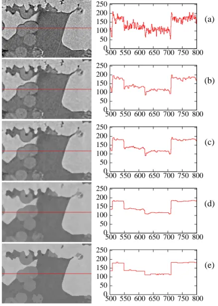
Fig. 3: Illustration of the image processing. In the left column a 2-d zoom in the sample (white rectangle in figure 2) undergoes the image treatment. The images are 300× 200 pixels with pixel size 0.28m. In the right column, a line of the zoomed image (noted in red in the left column) is plotted (pixel coordinate in abscissa, grey level in ordinate). From top to bottom: (a) the original image; (b) after step 1 of the ASF; (c) after step 2, (d) after step 3, (e) after the computation of the mosaic. The histograms of the whole 3-d image at each steps are visible on figure 4. The ASF clearly removes the noise in the image without blurring the borders between the phases. The watershed operation flattens more the image, yielding a very simple image to threshold.
0 5e+06 1e+07 1.5e+07 2e+07 2.5e+07 3e+07 0 50 100 150 200 250 Original ASF Mosaic
Fig. 4: Evolution of the histogram of a 1024× 1024 × 1024 voxels image during the
image processing. The starting image is visible on figure 6. Original is the histogram of the original images (figure 3-(a)), ASF after the ASF (figure 3-(d)) and Mosaic after the watershed (figure 3-(e)). In the starting image, the noise precludes any thresholding, the peaks are not distinguishible. The ASF makes them become visible, the watershed operation provides an increased clean-up of the image, resulting in the last histogram where the threshold levels are straightforward.
Fig. 5: Illustration of the segmentation. In the left column two 2-d zooms (300× 200
pixels) of the 3-d sample before image treatment. In the right column the thresholding of the mosaic, with levels selected using its histogram (minimum values between the three peaks); in black the porosity, in blue the silica, in yellow the calcite. In the top row, the image of figure 3, below a zone containing micritic calcite. This last example clearly shows that the smaller structures of the micritic calcite are lost, because of the ASF. However, some small zones appear in this image. It is due to the fact that the treatment of the image is fully 3-d while only a 2-d sample is here presented. These are small 2-d traces of a bigger 3-d structure.
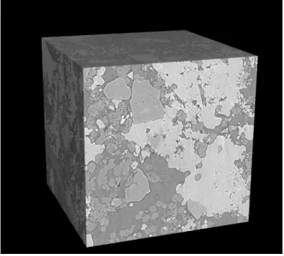
Fig. 6: 3-d illustration of the segmentation process: original image. The image is 1024×
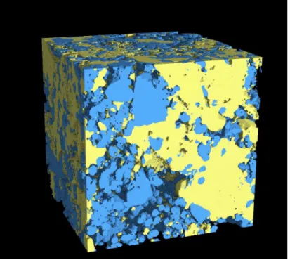
Fig. 7: 3-d illustration of the segmentation process: segmented version of the image in figure 6.