HAL Id: hal-01691703
https://hal.archives-ouvertes.fr/hal-01691703
Submitted on 24 Jan 2018HAL is a multi-disciplinary open access archive for the deposit and dissemination of sci-entific research documents, whether they are pub-lished or not. The documents may come from teaching and research institutions in France or
L’archive ouverte pluridisciplinaire HAL, est destinée au dépôt et à la diffusion de documents scientifiques de niveau recherche, publiés ou non, émanant des établissements d’enseignement et de recherche français ou étrangers, des laboratoires
Multicommodity flow problems with a bounded number
of paths : a flow deviation approach
Christophe Duhamel, Philippe Mahey
To cite this version:
Christophe Duhamel, Philippe Mahey. Multicommodity flow problems with a bounded number of paths : a flow deviation approach. Networks, Wiley, 2007, Multicommodity Flows and Network Design, 49 (1), pp.80-89. �10.1002/net.20143�. �hal-01691703�
Multicommodity flow problems with a bounded
number of paths : a flow deviation approach
Christophe Duhamel, Philippe Mahey
∗March 22, 2005
Abstract
We propose a modified version of the Flow Deviation method of Fratta, Gerla and Kleinrock to solve multicommodity problems with minimal conges-tion and a bounded number of active paths. We discuss the approximaconges-tion of the min-max objective function by a separable convex potential function and give a mixed-integer non linear model for the constrained routing problem. A heuristic control of the path generation is then embedded in the original al-gorithm based on the concepts of cleaning the quasi inactive paths and the reduction of the flow width for each commodity. Numerical experiments show the validity of the approach for realistic medium-size networks associated with routing problems in broadband communication networks with multiple proto-cols and label-switched paths (MPLS).
Keywords: Multicommodity flow, routing, flow deviation
∗Laboratoire d’Informatique, de Mod´elisation et d’Optimisation des Syst`emes,
UMR 6158 CNRS, Universit´e Blaise Pascal, Campus des C´ezeaux, Aubi`ere, France, email:{christophe.duhamel,philippe.mahey}@isima.fr
1
Introduction
We will consider a network routing problem with multiple pairs of origins and des-tinations where we want to minimize the maximal relative congestion on the arcs of the network under the restriction that the number of paths used to carry the traf-fic is bounded. The problem of minimizing the flow on the most congested link is of valuable interest for the design of data communication networks (see [4]). This basic problem is known to be hard to solve even if it can be written as a linear pro-gram. When additional constraints are present in the model, like path restrictions as considered here, it will result in very difficult problems for which exact methods are likely to be useless (see [15] for instance).
The particular path restriction we consider here is that the number of paths which support any feasible commodity flow is bounded by a given number (possibly de-pending on the commodity). Of course, when that number is equal to 1, we get the classical and difficult non bifurcated routing problem of unsplittable flows as de-noted by Kleinberg [13], and when the number is very large, we obtain the relatively easier routing problem with any flow splitting allowed. The intermediate situation considered here is of practical interest when dealing with label switched paths (LSP) in modern broadband communication networks. Indeed, in multiple protocol label-switched networks (MPLS) like all-optical IP backbones, different LSP are allowed to support the traffic for a given pair of nodes, but too many LSPs will deteriorate the performance of the protocols. One should thus try either to minimize the total number of LSPs (thus minimizing the number of wavelength conversions) with ad-ditional delay bounds to avoid congestion (see [3]) , or to minimize the congestion with bounds on the number of supporting LSPs. Observe that the first choice turns to be much more intricated as it includes the problem of searching a minimal set of paths to carry a given feasible flow, which is purely combinatorial. This is why we focus here on the second choice.
We will analyze here the adaptation of the Flow Deviation algorithm for Net-work Routing (see [4]) to this constrained minimal congestion problem. As the Flow Deviation method was designed to solve multicommodity flow problems with separable convex costs, we will show first how the maximal congestion cost func-tion can be approximated by these nonlinear funcfunc-tions, following earlier approaches based on polynomial approximation schemes and potential functions (see Bien-stock’s book for a comprehensive state-of-the art, [6]).
The Flow Deviation will be briefly surveyed in section 3, with emphasis on the path flow updates. In section 4, the routing model with a bounded number of paths will be established and different heuristic procedures will be proposed. These algorithmic issues will be validated in the last section.
2
Minimal congestion problems and potential
func-tions
In the remainder, we will callactivea path carrying a positive path flow.
Let G= (V, E) be a directed graph such that V is the set of nodes with |V | = n,
and E is the set of arcs with|E| = m. Each arc is assigned a capacity Ce, e ∈ E, and
T is a traffic requirement matrix such that, for each pair(i, j) of nodes, ti jrepresents
the amount of traffic required from node i to node j. Each pair of nodes such that
ti j> 0 will be referred to as a commodity and the index k will be associated with a
commodity, i.e. a pair of origin and destination nodes (respectively ok and dk), and
a traffic requirement tk= tokdk. The total flow on a given arc e∈ E will be denoted
by xe=∑kxkewhere xke is the amount of commodity k routed on arc e. In the
node-arc formulation of the multicommodity flow problem, we will need the node-node-arc incidence matrix A, (where aie= +1, aje = −1, if e = (i, j) ∈ E) to express the
individual flow constraints as Fk= {xk ∈ IRm| Axk= bk, xk≥ 0}, where
bki = +tk if i= ok −tk if i= dk 0 otherwise
The basic problem of minimizing the most congested arc in the routing of a multicommodity flow consists in minimizing the piecewise linear convex function
f(x) = maxexcee. The problem may nevertheless be modelled as a linear program by
adding an additional variable z as described below :
(MINCONG) min z s.t. ( ∑ k xke−Cez≤ 0, ∀e ∈ E xk∈ Fk, k= 1, . . ., K
Even if it is a linear multicommodity flow problem, thus an LP which can be solved by standard decomposition techniques exploiting the underlying flow struc-ture, it is generally considered a hard problem. The first reason why this occurs is that the objective function f is convex piecewise linear and not separable with re-spect to arcs. The second reason is that it produces optimal solutions with a large number of active paths, being in that sense equivalent to the Maximum Concurrent Flow problem as shown below. Bienstock has reported in [6] a set of numerical experiments on very large maximum concurrent flow problems (with up to 4• 105
rows and 2• 106columns) exhibiting abnormal cubic growth of the cpu time to solve them with the CPLEX dual code.
Observe that (MINCONG) is formulated without explicit capacity constraints on the total arc flows. This means that, besides its natural applications to congestion control in data networks, the routing problem (MINCONG) may be considered as an optimization formulation of the multicommodity flow feasibility problem, as we have the following relations : (MINCONG) is feasible if and only if there exists at least one path linking each origin to its destinations. Let z∗ be an optimal value for (MINCONG); there exists a feasible multicommodity flow if and only if z∗≤ 1.
The path structure of an optimal solution of (MINCONG) can be analyzed by considering its arc-path formulation. Let Pkbe the set of paths linking origin okwith
destination dkand xk pbe the path flow flowing on path p∈ P k, i.e. xk pis the portion
of the demand tkrouted on path p. The arc-path version of (MINCONG) is then :
(PCONG) min z s.t. ∑ k p;e∑∈pxk p−Cez ≤ 0 e∈ E ∑ p∈Pk xk p = tk k= 1, . . ., K xk p ≥ 0 k= 1, . . ., K, p ∈ Pk
We recall that a path is active when it carries some positive flow; an arc e will be calledcritical when it corresponds to the maximal congestion, i.e. when xe= Cez.
An active path containing critical edges will be called a critical path. Suppose now that some commodity is routed on a critical path p at the optimal solution and that there exists a second active path p0supporting that commodity which is not critical. Both paths define a cycle, so that one can modify the solution deviating a small quantity from p to p0. A new basic optimal solution should be obtained when p0
turns to be critical. That situation can thus only occur when there are multiple optimal solutions, else :
Proposition 1 Suppose (PCONG) has a unique optimal solution; then, if any
com-modity is routed on a critical path in an optimal solution of (PCONG), then all paths used to route that commodity are critical.
An optimal solution to (PCONG) will contain at most K+σ active paths (and at least K), whereσis the number of critical edges.
As observed in [21], (MINCONG) is also strongly related to the Maximum Con-current Flow problem (MAXTHRU), where one wants to maximize the throughput of the network for a given set of capacities. The throughput Z of the network is a load factor that multiplies the traffic matrix. In the model shown below, Xk repre-sents again the k-th commodity flow :
(MAX T HRU ) max Z
s.t. ( ∑ k Xek ≤ Ce Xk ∈ Fk(Z) k= 1, . . . , K where Fk(Z) = {Xk∈ IRm| AXk= Zbk, Xk≥ 0}.
One can easily verify that, for any optimal solution x∗ of (MINCONG), with optimal value z∗, there exists an optimal solution X∗of (MAXTHRU), with optimal value Z∗, such that x∗= z∗X∗and z∗= 1/Z∗. Moreover, the crucial fact is that both problem solutions share the same set of active paths.
Both problems (MINCONG) and (MAXTHRU) have received a lot of attention in the past decade, namely since the seminal paper by Shahrokhi and Matula [21] who first proposed a fully polynomial approximation scheme to solve (MAXTHRU) with uniform capacities. They showed that the minimization of a separable expo-nential penalty function on the arcs yields a flow with a nearly maximal throughput. They chose the following penalty function :
φe(xe) = exp(
2m2
where ε is a positive parameter which defines the approximation. They found a complexity bound of O(nm7/ε5) and showed that the number of active paths is in O(m3/ε2). Faster algorithms based on refinements of that exponential penalty
func-tion have been proposed later and extended to non uniform capacities and to other packing and covering problems (see [17], [12], [11]). Following Bienstock in [6], we will denote these separable penalty functions by the term ofpotential functions.
3
The flow deviation method
The Flow Deviation method (FD) is an adaptation of the classical linearization algo-rithm of Frank and Wolfe [9] to solve multicommodity flow problems with convex costs. It has been first proposed by Fratta, Gerla and Kleinrock [10] in the context of designing packet-switched networks and has been widely used by the transporta-tion community (see [16]) and in telecommunicatransporta-tions networks (see [4]). We recall below the formal ideas behind Frank-Wolfe’s algorithm for general nonlinear pro-grams with linear constraints :
Minimize Φ(x)
s.t. Ax= b x≥ 0
The method proceeds by successive linearization solving LP subproblems at each iteration t where the gradient ∇Φ(xt) has been computed. Let ˜xt be the optimal
solution of the subproblem at iteration t ˜
xt= Argminx∈P∇Φ(xt) • x
where P= {x ∈ IRn| Ax = b, x ≥ 0} is the polyhedron of feasible solutions supposed
bounded. Thus, we can assume that ˜xt is an extreme point of P. The direction dt=
˜
xt− xt is a descent direction in the sense that the directional derivative∇Φ(xt) • dt
is strictly negative. Then the new iterate is obtained by carrying out a line search on the segment[xt, ˜xt] with the non linear functionΦ. Convergence results have been
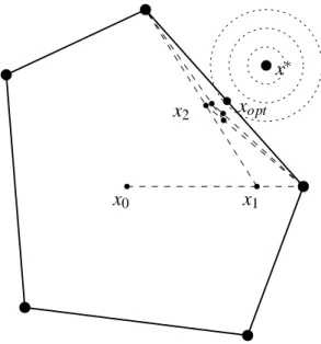
obtained in the strictly convex case (see [5] for example) but the method suffers from very slow convergence tail which is evidenced by the following fact : the solution of the non linear program is in general not a vertex of the feasible polyhedron so
that, as the sequence of feasible solutions converges towards a point on a face of the polyhedron, the angle between successive descent directions tends to 180◦(see Fig. 1). It is shown in [5] how typical sublinear convergence rate can be exhibited in very simple and low-dimensional situations. This drawback is somehow compensated by the observed fact that nearly optimal solutions typically within 1% of optimality -can be obtained very quickly.
x2
x1 x0
xopt
x∗
Figure 1: Zigzagging convergence of Frank and Wolfe’s method
On the other hand, the positive aspect of the implementation of Frank-Wolfe’s method to multicommodity flow problems is the simplicity of the subproblems res-olutions which reduce to shortest-path computation and the solution update which consists in fairly deviating flows from the active paths towards the new ones without explicitly computing the individual commodity flows as we can see below.
Now, to apply the Flow Deviation method to (MINCONG), we need to approx-imate the non smooth congestion function f(x) = maxexe/Ce by a smooth convex
function. This can be done by using a separable potential function as shown in the former section. An interesting link between the Flow Deviation algorithm and the resolution of (MINCONG) has been analyzed recently by Bienstock and Raskina in [7]. They proposed an algorithm to solve (MINCONG)which alternates between a magnification step where the throughput is increased for a fixed congestion and
a potential reduction step where congestion is minimized for a fixed throughput. That latter step is realized by performing flow deviation inner steps with the Klein-rock’s congestion function used in [10]. The interesting fact is that this function has an interpretation as a measure of the Quality of Service (QoS) of the network. It is indeed the average delay suffered by a data packet on arc e. In [10], indepen-dence assumptions with Poisson arrivals on the queuing network lead to Kleinrock’s delay function which is proportional to Φe(xe) = Cex−xe e. The total cost is simply
Φ(x) =∑eΦe(xe). Observe that the objective function acts as a barrier function on
the capacity constraints which can thus be ignored in the model :
Minimize Φ(x)
s.t. xk∈ Fk, k = 1, . . ., K
where Fk= {xk∈ IR|E|| Axk= bk, xk≥ 0} is the set of flows for commodity k.
Assume that we get a strictly feasible multicommodity flow at iteration k, i.e. such that xe < Ce, ∀e. Then, the linearization step of (FD) reduces to separate
shortest-path computations for each commodity k with arc lengths ∇Φe(xte). The
solution ˜xt corresponds to the situation where all demands tk are routed separately
on these new paths. Note that ˜xt may not satisfy the capacity constraints. The new solution xt+1 is obtained by carrying out a line search on the segment[xt, ˜xt]. Note
again that the new solution will be forced to strict feasibility by the barrier function. The main point in the procedure above is the fact that all computations are per-formed on the total flow variables. However, in some situations, one may be inter-ested in computing the optimal path flows. An arc-path formulation is then neces-sary and the (FD) iterations can be carried out on the path flow variables as explained in [4]. The first step of the procedure is unchanged so that, if ˜p is the shortest path
with the first-derivative arc lengths for a given commodity k, then we set ˜xk ˜p= tkand
˜
xk p= 0 for p 6= ˜p, so that the flow deviation step can be computed in the following
way :
xtk p+1= xtk p+θt( ˜xtk p− xtk p), ∀p ∈ Pk
where θt is the optimal step size which minimizes the objective function over all
θ∈ [0, 1]. As mentioned before, the method is a descent algorithm so that the values
Φ(xt) decrease monotonically. On the other hand, we can obtain easily a lower
( ˜xt− xt); these succesive values need not increase monotonically, so we must keep
the highest value as the current lower bound
LBt= max h=1,...,t
˜
LBh
In the original (FD) method, an equal fraction of the flow on the nonshortest paths is shifted to the shortest path. One may observe that this update of path flows will tend to increase monotonically the number of active paths. Variants of the basic Flow Deviation method can be built by modifying one of the inner steps of the algorithm, i.e.
• either by modifying the search direction, for instance by substituting the
shortest-path calculations by min-cost flow subproblems for each commodity,
• or by deviatingnon uniformflow proportions on the newly generated paths.
To understand the first strategy, one can add the redundant constraints xke≤ Ce, ∀e, k
to the model (MINCONG); after the linearization, the direction-finding subproblem of (FD) decomposes now in K minimum-cost flow problems. The computational overhead of these subproblems compared to the original shortest-path calculations is compensated by the choice of feasible paths (considering one commodity at a time). But the drawback is that more paths are likely to be generated which is ex-actly what we do not wish, and the path flow updates are not so straightforward as in the original method. Our testing with that variant has confirmed these difficulties and we had to decide not to implement it in our algorithm. Observe nevertheless that some authors have chosen to implement min-cost flow computations instead of shortest-path calculations to improve the worst-case behaviour of some approxima-tion algorithms (see [12] or [20]).
There are many different strategies to modify the search direction which result in non uniform deviations from the current active paths to the shortest one. Second-order information can be used to yield Newton or Quasi-Newton directions as sug-gested in [4]. Conjugate gradient strategies have also been tested in earlier works (see [14]). Again, the expected gain in convergence rate is overtaken by the extra work of performing each iteration and reconstituting the path support.
We will discuss in the last section heuristic procedures to carry out (FD) steps with a bounded number of paths.
4
Bounding the number of paths
We will finally consider a more complex but realistic situation where some path constraints are added to the (MINCONG) model. A way to find an interesting com-promise between low congestion and unsplittable flow is to add some constraints on the number of active paths for each commodity. The general case has been scarcely considered in the literature, the research focussing mainly on the very special cases where either a single path is forced for each commodity or two disjoint paths are required for security reasons (see Kleinberg’s thesis [13] for example). Another in-teresting type of constraints is the case of k-splittable flows where each commodity flow may be splitteduniformlyamong k routes [2]. Besides these studies, approxi-mation and heuristic techniques have been devoted to the reduction of the number of supporting paths with a linear or non linear objective function (see [8], [18], [19]).
Let Rk, k = 1, . . ., K be the maximum number of paths on which commodity k
can be routed. Thus a feasible routing is a set of Rk paths chosen in the set Pk
for each k such that ∑Rk
p=1xk p = tk, k = 1, . . . , K. It can be referred to as a (non
uniform) k-splittable flow, following Skutella and others. In [18], additional straints on the size of the trunks (path capacities) are considered. We will not con-sider these constraints here but instead use the congestion objective function dis-cussed in the previous sections. These problems are all known to be NP-complete as soon as Rk is lower than the number of paths supporting the optimal solution of
(PCONG). A mixed-integer programming formulation can be formalized to model the bound on the number of paths, introducing 0-1 variables associated with each path in (PCONG) : (BPCONG) min z s.t. ∑ k p;e∑∈pxk p−Cez ≤ 0 e∈ E ∑ p∈Pk xk p = tk k∈
K
xk p− tkyk p ≤ 0 k∈K
, p ∈ Pk ∑ p∈Pk yk p ≤ Rk k∈K
xk p ≥ 0 k∈K
, p ∈ Pk yk p ∈ {0, 1} k∈K
, p ∈ Pkcalled the flow width. If one solves a capacitated multicommodity flow problem with linear costs, the total number of active paths at the solution is at most K+ m, and,
supposing K = O(m), this results in an average of 2 active paths per commodity.
In practice, unfortunately, many commodities will be routed on a single path and a few of them will spread their flow on a large number of paths. Now considering an uncapacitated model with a nonlinear barrier function as above, the flow width at the optimal solution can be bounded thanks to Caratheodory’s theorem by m+ 1 for
each commodity. This is still a too large number and, even worse, the behaviour of the (FD) procedure will tend to add more paths than necessary in the construction of the current solution. Indeed, supposing one new path is generated at each iteration, as the procedure deviates flow in equal proportion from all active paths to these new ones, the flow width will monotonically increase with the iteration count. This nasty fact could be avoided at the cost of eliminating redundant paths in the definition of the current solution as a convex combination of path flows. Typically, pivoting steps are needed to compute the smallest representation in term of path flows.
The question we address here is how to maintain a limited number R of paths in the (FD) process. The difficulties to achieve this goal are :
• Global optimality will in general be far out of reach because most situations
will result in NP-hard problems;
• the arc-path model being implicit, we can only reroute the flows issued from
the cancelled paths towards the already generated paths;
• feasibility issues turn to be crucial as one does not know if the network will
be able to support the traffic on a smaller number of paths.
The central idea to approximately solve (BPCONG) is to adapt the Flow De-viation (FD) to the case of k-splittable flows. One can observe that the same idea has been used very early in the seminal paper by Fratta, Gerla and Kleinrock [10] who applied it to the particular case of unsplittable flows (Rk= 1, ∀k). The heuristic
procedure simply tries to deviate all the demand on the newly generated shortest paths without violating any capacity constraint. This can be performed commodity per commodity until no improvement in the objective function is observed. It seems clear that that simple method can stop too early with a very poor feasible solution unless the traffic load is very low. Besides that, the major problem with the adapta-tion of (FD) to k-splittable flows is the accumulaadapta-tion of active paths in the iterative
process. Indeed, the flow is deviated in equal proportions from all current paths to load the new one and, either all previous path flows are set to zero (θt= 1) or all are
decreased (0<θt < 1) and the flow width increased by one unit, the latter situation
being the most likely to occur. Now observe that the general problem to find a set of paths supporting a given feasible flow has in general many solutions. Indeed, if Mk is the arc-path incidence matrix associated with the set Pkt+1 of paths for the
k-th commodity after updating the flows at iteration t and xt+1 (resp. ft+1) is the path flow vector for the new active paths (resp. the arc flow vector), we look for a solution of the following linear system :
M1 · · · Mk · · · MK eT . .. eT . .. eT xt+1= ft+1 d1 .. . dk .. . dK
where e is a vector of 1. This system always possess at least one solution with non negative components (the one which corresponds to the classical uniform deviation and used all paths in the current representation), but we should be able to find a better solution using less paths for the same arc flow values. Unfortunately, the problem to find a minimum supporting path set for a given flow, i.e. to compute the minimal flow width, is NP-hard (see [22]). Moreover, the indetermination in the definition of the path support is more intricate in the case of multicommodity flows as, for a given feasible multicommodity flow, there are in general an infinity of individual arc flow solutions which satisfy the multicommodity flow constraints ∑kxke= xe, ∀e ∈ E. For
a single positive flow on a directed graph, the flow decomposition theorem (see [1]) guarantees there exists a support with at most n+ m paths and cycles (and at most m cycles). When the only directed cycles in the network are the ones which use the
return arc from the sink back to the source, it can be easily seen that the minimum number of active paths is bounded above by m− n + 2 (using paths with linearly
independent incidence vectors). But this number will in general be too large to be of practical interest as network protocols do not allow for a splitting in more than, say, 10 paths, even in large dense networks.
The basic ingredients of our procedure are :
Cleaning the poorest routes: the cleaning procedure is based on the idea that some
the flow deviation procedure will decrease the amount of flow but will still maintain a positive quantity of flow on these routes. Thus a first strategy to reduce the number of paths consists in canceling the paths which support a quantity of flow which is less than a given relative threshold. The solution is then updated, either by optimizing the cost on the corresponding reduced set of paths before generating any new path, or by fairly sharing the canceled quantity of traffic on the remaining paths. Observe that the new objective function value can have increased during that phase, but in most situations, the canceled paths will not be active any more in the future solutions, including the optimal one.
Iterative loading of commodities: a second strategy, already mentioned in the case
of unsplittable flows, consists in updating the flow one commodity at a time. This can be interpreted as a Gauss-Seidel like version of the Flow Deviation method, where the line-search is performed on a single commodity flow. As a consequence, the stepsizeθwil be greater and more path flows will decrease significantly with a higher probability to be canceled.
Avoiding unprofitable shortest path calculations: in the original (FD) algorithm,
a shortest path is computed for each commodity at each iteration. However, com-putational experiments show that, most of the time, the new shortest path already belongs to the current solution set of active paths. Only few brand new improving paths are identified during the optimization (typically, less than 100 paths are stored at the end of several thousands FD iterations). Then, it may be interesting to try to look for an improving path among the active paths instead of computing a shortest path. We have modified the improving path selection in the following way : during a given number τ of iterations, the improving path is computed among the active paths. At the begining, τ← 10. Then, at the end of the minor iterations, a shortest
path is computed. If this path is also an active one, thenτ← 2τotherwiseτ← 10.
Controlling the flow width: there are two ways to control the flow width for each
commodity. The first one (external) is based on relaxing first the width constraint, then trying to satisfy it progressively. The second one (internal) keeps the width constraint during the flow deviation procedure. In the external procedure, the width constraint is restored using the same idea as in the cleaning procedure. At each iteration of the restoration, the active path with the smallest amount of flow is fairly rerouted among the remaining ones, then a flow deviation with τ←∞ is applied to locally optimize the flow structure. A path control is added at each step in the internal procedure : once a flow reaches its width limit, τ←∞, if its width drops
below the limit, thenτ← 10.
5
Numerical experiments
The (FD) algorithm and its variants adapted to problem (BPCONG) have been coded in C and compiled through gcc 3.2 on the gnu/linux system. The numerical tests were performed on an Intel P3 800 MHz computer with 256 Mb RAM.
Test networks: The test networks used for the numerical experimentation are of
two types : 1) a realistic core network instance with 12 nodes, 88 arcs and 74 com-modities; 2) a testbed of 20 random instances; those instances are built on planar graphs (obtained through Delaunay triangulation) whose size ranges from 10 to 40 nodes. For each size, 5 different sets of demands have been randomly defined. The number of commodities has been set to 2n, 4n, 6n, n(n − 1)/2 and n(n − 1) where n
is the number of nodes.
Initialization procedure: flow deviation needs an initial solution. Thus, one has to
provide a way to compute a feasible solution. This is achieved through the following heuristic, denoted by INITFD. It first consists in cutting all demands into equal-sized packets. Then each packet is routed, one at a time, on the shortest path where arc costs are the load first derivative. Arc loads are updated after each packet has been sent. Packets are randomly chosen from the remaining ones at each iteration to prevent bias and ill behaviour. However, this is not sufficient to guaranty feasibility of the solution since wrong routing decisions may be made. In practice, when the network is not close to saturation, those problems are not likely to appear.
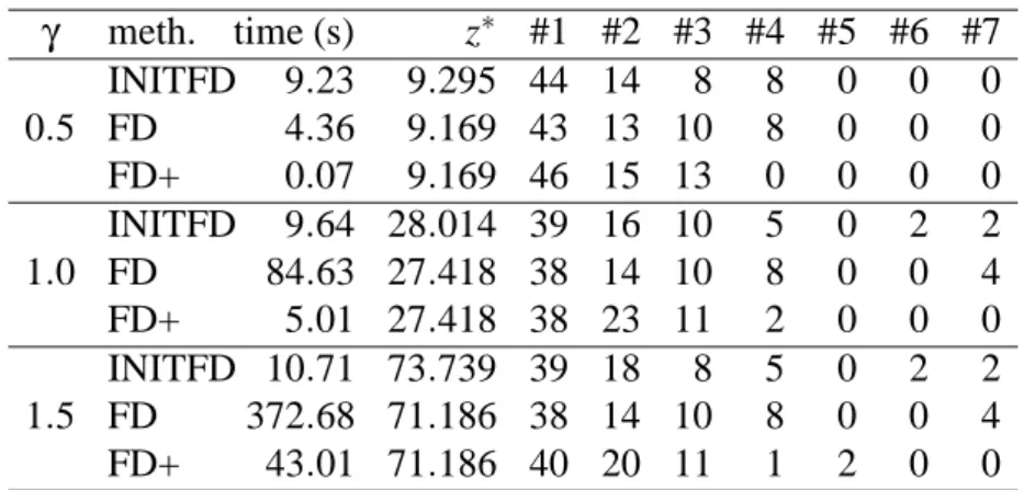
In Table 1, results are shown for varying values of the throughputγ(a common multiplying factor for all commodities demand). INITFD, FD and FD+ rows re-spectively give informations for the heuristic, the classical flow deviation method and the flow deviation method using the cleaning procedure and the improved path generation. For each method and eachγ, CPU time in seconds, value of the optimal solution are reported. The last seven columns give the number of commodities in the solution with the given number of active paths. The cleaning procedure (FD+ method) helps a lot reducing the number of active paths. Combined with the modi-fied path generation, they also provide a strong reduction in CPU time. The reason is that the cleaning procedure removes paths that are not likely to be in the optimal
γ meth. time (s) z∗ #1 #2 #3 #4 #5 #6 #7 INITFD 9.23 9.295 44 14 8 8 0 0 0 0.5 FD 4.36 9.169 43 13 10 8 0 0 0 FD+ 0.07 9.169 46 15 13 0 0 0 0 INITFD 9.64 28.014 39 16 10 5 0 2 2 1.0 FD 84.63 27.418 38 14 10 8 0 0 4 FD+ 5.01 27.418 38 23 11 2 0 0 0 INITFD 10.71 73.739 39 18 8 5 0 2 2 1.5 FD 372.68 71.186 38 14 10 8 0 0 4 FD+ 43.01 71.186 40 20 11 1 2 0 0
Table 1: cleaning procedure and improved path generation (γinfluence) solution. Thus, removing those suboptimal paths avoid a lot of iterations that would otherwise be needed to reduce their amount of flow down to zero.
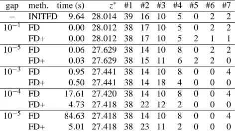
Table 2 shows the impact of the required final gap (column “gap”) on the FD and FD+ methods. The meaning of the columns is the same as before. It can be clearly seen that the cleaning procedure and the internal path generation help keeping low CPU time as well as providing solutions with a low number of path per commodity. This also suggests the fact that FD+ as a better experimental convergency towards the optimal solution.
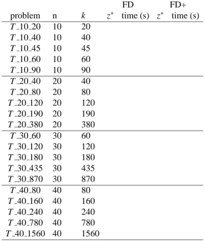
Table 3 summarizes the behaviour of FD and FD+ for the whole set of instances. Again, FD+ compares well against FD. BLABLABLA `a ajouter
Table 4 illustrates the path control procedure on the optimal solution. The first column shows the width upper bound R for every commodities. In all cases, flow
gap meth. time (s) z∗ #1 #2 #3 #4 #5 #6 #7 − INITFD 9.64 28.014 39 16 10 5 0 2 2 10−1 FD 0.00 28.012 38 17 10 5 0 2 2 FD+ 0.00 28.012 38 17 10 5 2 1 1 10−5 FD 0.06 27.629 38 14 10 8 0 2 2 FD+ 0.03 27.629 38 15 11 6 2 2 0 10−3 FD 0.95 27.441 38 14 10 8 0 0 4 FD+ 0.50 27.441 38 14 18 4 0 0 0 10−4 FD 17.61 27.420 38 14 10 8 0 0 4 FD+ 4.73 27.418 38 22 12 2 0 0 0 10−5 FD 84.63 27.418 38 14 10 8 0 0 4 FD+ 5.01 27.418 38 23 11 2 0 0 0
Table 2: cleaning procedure and internal path generation (gap influence)
deviation with internal path management (FD+int) requires less CPU time than flow deviation with external path management (FD+ext). There are two reasons: first, when FD+int reaches some commodity width limit, it is quite difficult to find an alternate path to exchange with an active one. Second, removing an active path in FD+ext does a lot of perturbation. The quality of the solution for both methods is nearly the same. No accurate gap can be produced since the only valid lower bound is unconstrained flow deviation lower bound.
Finaly, the last table shows flow deviation behaviour for the unsplittable case that is, when R= 1. We compare flow deviation with internal path management
(FD+int) against two heuristics. H1 (resp. H2) sorts the commodities by decresing (resp. increasing) demands and then route each one on the shortest path, where the cost are the delay first derivative. Those costs are updated after each routing. It can be seen H1 is quite close to FD for a much lesser CPU time. This shows the limits of our approach, when the width constraint is very low.
FD FD+ problem n k z∗ time (s) z∗ time (s)
T 10 20 10 20 T 10 40 10 40 T 10 45 10 45 T 10 60 10 60 T 10 90 10 90 T 20 40 20 40 T 20 80 20 80 T 20 120 20 120 T 20 190 20 190 T 20 380 20 380 T 30 60 30 60 T 30 120 30 120 T 30 180 30 180 T 30 435 30 435 T 30 870 30 870 T 40 80 40 80 T 40 160 40 160 T 40 240 40 240 T 40 780 40 780 T 40 1560 40 1560
Table 3: results for the random instances
R meth. time (s) z∗ #1 #2 #3 #4 no FD 5.03 27.418 38 23 11 2 3 FD+int 1.90 27.438 38 26 10 0 FD+ext 8.53 27.418 38 29 7 0 2 FD+int 9.47 27.478 40 34 0 0 FD+ext 33.38 27.478 39 35 0 0 1 FD+int 12.05 39.608 74 0 0 0 FD+ext 15.41 39.608 74 0 0 0
starting solution integer flow FD heur. value time (s) value time (s)
H1 39.614 0.00 39.577 0.00
H2 175.509 0.00 39.575 0.01
FD+int 39.608 12.05
Table 5: unsplittable flow
6
Conclusion
The Flow Deviation algorithm remains a very versatile and prolific tool to solve routing and design problems in networks since the pioneer work of M. Gerla in the seventies. Several variants and algorithmic improvements have been proposed and validated here to take in consideration some bounds on the number of active paths to support the less congested solutions. As the resulting model leads to NP-hard problems for most practical situations, heuristic have been first proposed to show how the simplicity of the Flow Deviation updates is very useful to control the number of paths for each commodity. Of course, extreme situations like the unsplittable situation associated with heavy loads are unlikely to yield nice results with these heuristics as the theoretical approximation bounds are known to be quite weak for these hard problems. In these cases, branching procedures and the efficient generation of valid cuts should be added to the basic (FD) iteration to get good solutions. These studies are currently under studies with a limited computational experience on small to medium-size networks.
References
[1] R. Ahuja, T. Magnanti, and J. Orlin. Network Flows : Theory and Algorithms. Prentice-Hall, Englewood Cliffs, 1993.
[2] G. Baier, E. K¨oehler, and M. Skutella. On the k-splittable flow problem.
[3] D. Banerjee and B. Mukherjee. Wavelength-routed optical networks : Lin-ear formulation, resource-budgeting tradeoffs and a reconfiguration study.
IEEE/ACM Transactions on Networking, 8(5):598–607, 2000.
[4] D. Bertsekas and R. Gallager. Data networks. Prentice-Hall, Englewood Cliffs, 1987.
[5] D. P. Bertsekas. Nonlinear Programming. Prentice-Hall, Englewood Cliffs, 1995.
[6] D. Bienstock. Potential Function Methods for Approximately Solving Linear
Programming Problems : Theory and Practice. Kluwer Publishers, 2003.
[7] D. Bienstock and O. Raskina. Asymptotic analysis of the flow deviation method for the maximum concurrent flow problem. Mathematical
Program-ming, 91:479–492, 2002.
[8] J. Burns, T. Ott, A. Krzesinski, and K. Muller. Path selection and bandwidth al-location in mpls networks : a non linear programming approach. Performance
Evaluation, 52:133–152, 2003.
[9] M. Frank and P. Wolfe. An algorithm for quadratic programming. Naval
Research Logistics Quarterly, 3:95–110, 1956.
[10] L. Fratta, M. Gerla, and L. Kleinrock. The flow deviation method: an approach to store-and-forward computer-communication network design. Networks, 3, 1973.
[11] N. Garg and J. K¨onemann. Faster and simpler algorithms for multicommod-ity flow and other fractional packing problems. In Proc. 39th Ann. Symp. on
Foundations of Computer Science, 1998.
[12] M. D. Grigoriadis and L. G. Khachiyan. Fast approximation schemes for con-vex programs with many blocks and coupling constraints. SIAM Journal on
Optimization, 4(1):86–107, 1994.
[13] J. Kleinberg. Approximation algorithms for disjoint path problems. PhD thesis, MIT, Cambridge, 1996.
[14] L. B. J. LeBlanc, R. Helgason, and D. Boyce. Improved efficiency of the frank-wolfe algorithm for convex network programs. Transportation Sci., 19:445– 462, 1985.
[15] L. B. J. LeBlanc, P. Mahey, and J. Chifflet. Packet routing in telecommunica-tions networks with path and flow restrictelecommunica-tions. INFORMS J. on Computing, 11:188–197, 1999.
[16] L. B. J. LeBlanc, E. Morlock, and W. Pierskalla. An efficient approach to solv-ing the road network equilibrium traffic assignment problem. Trans. Research, 3:309–318, 1975.
[17] F. T. Leighton, F. Makedon, S. Plotkin, C. Stein, E. Tardos, and S. Tragoudas. Fast approximation algorithms for multicommodity flow problems. Journal of
Computer and System Sciences, 50(2):228–243, 1995.
[18] M. Martens and M. Skutella. Flows on few paths : algorithms and lower bounds. In Proc. 12th Annual European Symposium on Algorithms, ESA’04, 2004.
[19] V. Mirrokni, M. Thottan, H. Uzunalioglu, and S. Paul. A simple polyno-mial time framework for reduced-path decomposition in multi-path routing. In Proc. INFOCOM, 2004.
[20] S. A. Plotkin, D. B. Shmoys, and E. Tardos. Fast approximation algorithms for fractional packing and covering problems. Mathematics of Operations
Re-search, 20(2):257–301, 1995.
[21] F. Shahrokhi and D. W. Matula. The maximum concurrent flow problem.
Jour-nal of the ACM, 37:318–334, 1990.
[22] B. Vatinlen, C. Duhamel, F. Chauvet, and P. Mahey. Minimizing congestion with a bounded number of paths. In Proc. Algotel’03, Banyuls, 2003.