D-branes and string field theory

D-branes and String Field Theory

by

Ilya Sigalov

Submitted to the Department of Physics

in partial fulfillment of the requirements for the degree of

Doctor of Philosophy in Physics

at the

MASSACHUSETTS INSTITUTE OF TECHNOLOGY

September 2006

@

Ilya Sigalov, MMVI. All rights reserved.

The author hereby grants to MIT permission to reproduce and

distribute publicly paper and electronic copies of this thesis document

in whole or in part.

Author ...

...

Department of Physics

*7

May

31,

ZUUo

/11

Certified by ... .

...

T l.or-.

/d

Washington Taylor

Professor of Physics

Thesis Supervisor

Accepted by ...

MASSACHUSETTS INSTIJTE OF TECHNOLOGY

JUL 02 2007

LIBRARIES

... .. .' ".r "-". • M ... .•o.

-T'homas

;ireytak

Associate Department Head for ducation

D-branes and String Field Theory

by

Ilya Sigalov

Submitted to the Department of Physics on May 31, 2006, in partial fulfillment of the

requirements for the degree of Doctor of Philosophy in Physics

Abstract

In this thesis we study the D-brane physics in the context of Witten's cubic string field theory. We compute first few terms the low energy effective action for the non-abelian gauge field A, from Witten's action. We show that after the appropriate field redefinition which relates the string field theory variables to the worldsheet variables one obtains the correct Born-Infeld terms. We then compute the rolling tachyon so-lution in the context of string field theory. We show that after the appropriate field redefinition we obtain the rolling tachyon solution of Sen.

Thesis Supervisor: Washington Taylor Title: Professor of Physics

Acknowledgments

I am very much indebted to my advisor Washington Taylor and my friend and collab-orator Erasmo Coletti for endless discussions and computations done together. I am grateful to fellow students Jessie Shelton, Ian Ellwood, Dmitry Sigaev, Umut Gur-soy, Maria Chan, Keith Lee, Claudio Marcantonini, Guido Festuccia and Antonello Scardicchio for numerous discussions and support. I would like to thank Dmitry Belov, Elena Goubankova, Barton Zwiebach, Ashoke Sen, Hiroyuki Hata, Gianluca Grignani, Martha Orselli, Valentina Forini and Guiseppe Nardelli for discussions and useful suggestions.

I am deeply grateful to my parents Lev and Rimma Sigalov my brother Boris and my girlfriend Elena Pyatov for support love and understanding whenever it was

Contents

1 Introduction 15

2 Abelian and nonabelian vector field effec

theory

2.1 Introduction...

2.2 Review of formalism ... 2.2.1 Basics of string field theory 2.2.2 Calculation of effective action 2.2.3 The effective vector field action a 2.3 Computing the effective action ...

2.3.1 Generating functions for terms ir 2.3.2 Effective action for massless field 2.3.3 Level truncation ...

2.4 The Yang-Mills action ... 2.4.1 Quadratic terms ... 2.4.2 Cubic terms ... 2.4.3 Quartic terms ... 2.5 The abelian Born-Infeld action..

2.5.1 Terms of the form 02A4 . 2.5.2 Gauge invariance and field

2.5.3 Terms of the form a4A4 2.5.4 Terms of the form A2n _.

redefil

tive actions from string field

21 . . . . 21 . . . . 24 . . . . . 24 . . . . . 26 nd Born-Infeld . ... 29 . . . . 33

the effective action .... . 33

s .. . . . 38 . . . . 41 . . . . 43 . . . . . . . . .. . 43 . . . .. . 44 . . . . . .. 46 . . . . . 48 . . . .. . 49 nitions . ... ... . . 53 . . . . 59 .. . . . . . . 62 2.6 The nonabelian Born-Infeld action ...

2.6.1

0

3_A3 _{terms ...}

2.6.2

&

2_A4 _{terms ...} 2.7 Conclusions ...

3 Taming the Tachyon

in Cubic String Field Theory

3.1 Introduction ... .. . ...

3.2 Solving the CSFT equations of motion . . . . 3.2.1 Computing the effective action . . . . 3.2.2 Solving the equations of motion in the effective 3.3 Numerical results ...

3.3.1 Convergence of perturbation theory at L = 2 . 3.3.2 Convergence of level truncation . . . . 3.4 Taming the tachyon with a field redefinition . . . . . 3.5 Discussion . . . . 77 . . . . .. 77 . . . . . 80 . . . . . 81 theory . . . . 84 . . . . 87 . . . . . 87 . . . . . 90 . . . . . 93 . . . . 99

4 Conclusions and future directions A Neumann Coefficients

B Perturbative computation of effective tachyon action

C Construction of A(wl, w2, w3) in the continuous case

101 103

107

List of Figures

2-1 Twists T, T' and reflection R are symmetries of the amplitude. . ... .

37

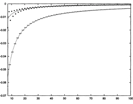
2-2 Deviation of the coefficients of quartic terms in the effective action from the ex-pected values, as a function of the level of truncation L. The coefficient -y+ is shown with crosses and y- - 1/2 is shown with stars. The curves given by fitting with a

power series in 1/L are graphed in both cases. . ...

47

3-1 The solution 0(t) including the first two turnaround points, including fields up to level L = 2. The solid line graphs the approximation 0(t) = et + c2e2t. The long dashed line graphs 0(t) = et + c2e2t + c3e3t. The approximate solutions computed up to e4t, e5t and e6t are very close in this range of t and are all

rep-resented in the short dashed line. One can see that after going through the first turnaround point with coordinates (t, 0(t)) - (1.27, 1.8) the solution decreases, reaching the second turnaround at around (t, 0(t)) - (3.9, -81). The function

f(o(t)) = sign(4(t))log(1 + |I(t)j) is graphed to show both turnaround points clearly on the same scale. ... 88

3-2 First turnaround point for the solution in L = 2 truncation scheme. The large plot shows the approximations with 03 (the gray line), 04 (black solid), and

k

5 (dashed lines) terms in the action taken into account. The smaller plot zooms in on the approximations with 4' and 05 terms taken into account. The corrections from higher powers of 0 are very small and the corresponding plots are indistinguishable from the one of the

45

approximation. . ... . 89

3-3 Second turnaround point for the solution in L = 2 truncation scheme. The gray line on the large plot shows the solution computed with the effective action including terms up to ¢4. The black solid and dashed lines represent higher order corrections. On the small plot the solid line includes 05 corrections, the dotted line includes corrections from the q6 term and the dashed line takes into account the 07 term.

3-4 The figure shows the convergence of the solution around the first turnaround point as we increase the truncation level. Bottom to top the graphs represent the ap-proximate solutions computed with the effective action computed up to 04 and

truncation level increasing in steps of 2 from L = 2 to L = 16. We observe that the turnaround point is determined to a very high precision already at the level 2. Similar behavior is observed for the second turnaround point ... 92

B-1 The first few diagrams contributing to the effective action . ... 108

B-2 To construct the 4 point diagram we label consecutively the edges of vertices on one hand and propagators and external states on the other. The matrix K corresponds to a permutation which glues them into one diagram. . ... 109

C-1

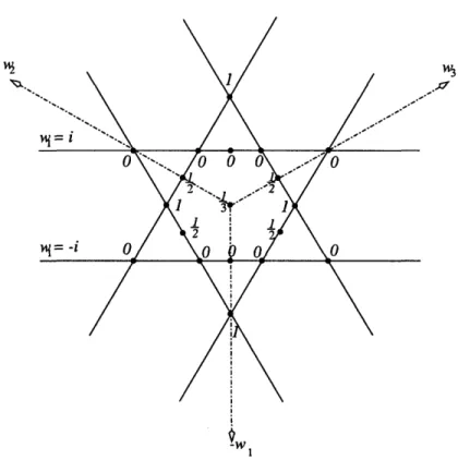
Construction of a continuous A(wi, w₂, w3): The figure shows the plane -wl +w2 +

w3 = 0 coincident with the plane of the paper. Dashed lines are the coordinate axes -w1, w2, w3, going at equal angles out of the plane of the paper. The two solid horizontal lines are intersections of the plane -w1 + w2 + w3 = 0 with the planes wi = ±i. According to (C.2) the function A is zero along these lines. Clearly, in

this projection the cyclic shift of momenta wi corresponds to a 60 degree rotation. Thus, the condition (C.1) implies that the sum of the values of A over the vertices of any equilateral triangle centered at the origin is one. Together with the reflection symmetry w2 + w3 this allows us to fix the value of A at several discrete points. The values are shown on the figure. The slanted solid lines show the locus of the vertices of equilateral triangles with one vertex fixed on the lines w2 _{= ±i. The} assignment of a value for A on one of the slanted lines defines the values on the other line, related by 600 rotation. These assignments can be made continuously along the lines while taking the values 0, 1, and - at the symmetrically positioned points. One can then continuously extend A into the rest of the plane, while maintaining (C.1) by interpolating between the values of A at the boundaries. . ... 114

List of Tables

2.1 Coefficients of the constant quartic terms in the action for the first 10 levels. . 47 2.2 Coefficients of A2n at various levels of truncation . ... 64

Chapter 1

Introduction

Modern physics classifies the observed forces of nature into four interactions: elec-tromagnetic, weak, strong and gravitational. Three of them: elecelec-tromagnetic, weak and strong have fully consistent quantum-mechanical description as specific quantum field theory with SU(3) x SU(2) x U(1) gauge symmetry. This quantum field theory, describes all three interactions within one framework. Together with specific data for particle spectra and fundamental constants it describes all observed accelerator particle physics.

The fourth interaction: gravitation has only classical description. It is also a gauge theory where the role of the gauge transformations is played by the reparametrizations of the space time. However, the quantization of gravity has proven to be extremely difficult problem. In the core of it is the issue of renormalizability of the quantum theory. When a classical field theory is quantized, say, via path integral methods the perturbative expansion of the observable quantities, such as scattering amplitudes, around the non-interacting theory is obtained. In this perturbative expansion indi-vidual terms are divergent, however for a class of QFT's via a careful and systematic procedure called renormalization, it was shown that the divergencies can be canceled out between the individual terms, contributing to each order in perturbation theory. While weak, strong and electromagnetic interactions have been shown to be renor-malizable, it was also found that the gravity, beyond the second order in perturbation theory, is not.

One more attractive physical idea which has been extensively explored is that of unification. It is known that electromagnetic, weak and strong interactions appear in the low energy limit of a class of larger quantum field theories with bigger gauge symmetry group. When going to the low energy limit, this large gauge symmetry is spontaneously broken and some of the gauge bosons receive masses, with the re-maining symmetry being SU(3) x SU(2) x U(1) of strong, weak and electromagnetic forces. The unified description is attractive because it uses less fundamental constants to specify the theory, and explains the family structure of the particle spectrum.

Probably one of the most challenging physics problems today is that of finding a unifying theory that would describe all four fundamental forces as one interaction, where the splitting into apparently different interactions would appear only in the low energy limit. Although gravitation is not renormalizable, in this context it would appear in the special regime of a bigger and self consistent theory. In the last 15 years string theory has become the most prominent candidate for such a theory.

The string theory's basic assumption is that instead of being pointlike objects, the elementary particles are extended objects - strings. Strings can be open or closed. While moving in spacetime a string spans a surface called the string worldsheet. Elementary particles with different quantum numbers appear as various string exci-tations as we look at strings from large distances. One of the very attractive features of this point of view is that different particles appear as different excitations of one fundamental string.

In mid-eighties it was found that in flat spacetime there are five consistent super-symmetric string theories, which must live in 10-dimensional Minkowski space. All of these theories are related by various duality transformations, and it is generally as-sumed, that these are different limits of unique fundamental theory. The connection to our 4-dimensional world is made via procedure called compactification, where 6 of the 10 dimensions are assumed to span some compact manifold. Excitation of the string in the compact direction would require large energies, leaving strings to move freely in the four spacetime dimensions.

of excited states in noninteracting theory are well defined, and scattering amplitudes are computed order by order in perturbation theory. All of the five formulations are related by so called duality transformations - which state that perturbative definition of one string theory appear in a specific regime of another. It was then assumed that these five apparently different string theories are perturbative expansions around different backgrounds of some fundamental underlying theory.

With the research that followed the seminal paper of Polchinski [2] the importance of D-branes in string theory has been fully realized. D-branes in string theory appear as localized D + 1 dimensional objects, whose perturbations are described by the open string degrees of freedom. Open strings are allowed to end on the D-brane only. Different open string backgrounds correspond to D-branes with different geometry. From the space time point of view, D-branes are classical solutions to the supergravity equations of motion.

An important question is to find a theory, which would possess a so called back-ground independence. Such theory should allow a description of different string models as different backgrounds specified in terms of some fundamental variable. Perturbative expansions around these backgrounds would give us the five string the-ories and their compactifications. Different D-brane configurations would also be described as open string backgrounds in the fundamental background independent theory. The best known candidate for the background independent formulation of string theory is String Field Theory (SFT). While there are SFT formulations for some of the 10-dimensional supersymmetric string theories, most significant progress in understanding different string backgrounds using string field theory was achieved in Witten's cubic string field theory (CSFT) which describes the 26-dimensional open bosonic string. The lowest state of 26-dimensional bosonic string has negative mass squared, which is the indication that the theory is unstable. Before the remarkable paper of Sen [1] it was assumed that the presence of the tachyon presents fundamental problems with open bosonic string. Witten's cubic string field theory (CSFT) pro-vided the action which describes the interaction of the tachyonic and all the excited states. From this action one can compute the effective potential for the tachyonic

state. Ashoke Sen in [1] has made three conjectures about the relationship between open string vacua with dramatically different geometrical properties:

1. The effective potential for the tachyon has a minimum, furthermore, the energy difference between the perturbative vacuum and the minimum of the tachyon potential is exactly the energy of the space-filling 25 dimensional D-brane. 2. In the perturbative expansion around the tachyonic vacuum there are no open

string excitations. The minimum of the tachyonic potential corresponds to the closed string vacuum where the D-brane has decayed and only closed string excitations are remaining.

3. The lower dimensional branes should be realized as the soliton configurations of the tachyon and other string excitations.

These conjectures have been verified by numerical computations in CSFT in [3, 4, 5, 6, 7, 8, 9, 10] as well as in subsequent research (see [11, 12, 13, 14] for reviews of this

work).

Sen's conjectures have made CSFT into an important tool for studying various string backgrounds. In my work with Washington Taylor and Erasmo Coletti we have concentrated on two aspects of string field theory. In Chapter 2, following [15] we describe the calculation of the low energy effective action of the 25-dimensional D-brane from CSFT. In the low energy limit there are two excitations of the open bosonic string remaining: the tachyon €, which has negative mass squared and the massless vector field A, which describes the perturbations of the D-brane. The gauge field A, takes values from U(n) group. From earlier work analyzing string scattering amplitudes and string partition function [16, 17, 18] it was known, that the low energy effective action for the U(1) vector field A, is so called Born-Infeld action

S = M)2

f

dx

-det

(T,, + 21gyMF•,) (1.1)

The lowest term in the power expansion of (1.1) is the usual electromagnetic action. It has also been assumed that for the U(n) models with n > 2 the resulting action

must be a non-abelian generalization of (1.1). The leading terms in the expansion of such action were computed by analyzing string scattering amplitudes and, in the supersymmetric case by the analysis of restrictions imposed by supersymemtry. The full form of the non-abelian vector field effective action is not known.

The development of SFT provided us with an alternative method of computation of effective action. In the work of Taylor [19], the first calculation of the vector field effective action from SFT was done, and it was shown, that in the abelian case, up to terms of order A2 the action is simply the standard electromagnetic term. Further progress in the computation of effective action was made with [20] where the method of computation of Feynman diagrams in string field theory was proposed. Using this method in [15] we have computed the effective action for abelian and non-abelian cases as the low energy effective action of string field theory up to terms of the order A4. We have also checked by numerical computation that non gauge invariant terms A" cancel for n > 4.

Probably the most important realization of [15] was that the variables in the world sheet and string field theory formulations of string theory are not the same, but rather related by a complicated field redefinition. In the worldsheet formulation of string theory the vector A, has standard gauge transformation from the start, and the resulting action is a function of the gauge invariant stress tensor F,, and it's derivatives.

In SFT, gauge invariance for A, is dictated by the gauge invariance of the string field theory. After the higher energy excitations are eliminated using the equations of motion, the gauge invariance for A, becomes rather complicated non-linear transfor-mation. The field redefinition is required to bring the gauge transformation into the standard form. Only after this field redefinition is made, do we obtain the Born-Infeld action in the U(1) case and in the U(n) case it's non-abelian generalization.

Another aspect of D-brane physics we study from string field theory point of view is the rolling tachyon solution of Sen [22]. The rolling tachyon solution is the string background which was proven by Sen to be exact solution of string field theory equations of motion. In Chapter 3 following [21] we solve the CSFT equations of

motion for the rolling tachyon initial condition. The initial condition for the tachyon (x, t) is specified by the asymptotics ¢(x, t) - et as t -+ -oo. The tachyon field is assumed to stay constant along the spatial coordinates. The motivation for this work comes from the works of Sen [22, 23, 24] on the rolling tachyon in worldsheet formulation of string theory and the work of Moeller and Zwiebach [25] where the rolling tachyon solution in CSFT was calculated in the level zero truncation (which basically means that the theory is truncated to include the tachyon field only, all other fields are forcibly set to zero). In [25] authors have found that the rolling tachyon solution in the level 0 truncation develops evergrowing oscillations. This picture is dramatically different from the worldsheet picture, where the worldsheet tachyon T(t) - et was shown by Sen to be exact solution. Moeller and Zwiebach conjectured that the situation might get amended by including massive string modes into consideration. We show in [21] that this is not the case, and in fact the growing oscillations are present in CSFT rolling tachyon solution even when we include the massive string modes. The apparent contradiction is resolved by the field redefinition T(O) which relates the worldsheet tachyon into the CSFT one. We compute the field redefinition to the leading order in power expansion in ¢ and show that it indeed maps the rolling solution of Sen into the CSFT rolling solution.

Chapter 2

Abelian and nonabelian vector

field effective actions from string

field theory

2.1

Introduction

Despite major advances in our understanding of nonperturbative features of string theory and M-theory over the last eight years, we still lack a fundamental nonper-turbative and background-independent definition of string theory. String field theory seems to incorporate some features of background independence which are missing in other approaches to string theory. Recent work, following the conjectures of Sen [1],

has shown that Witten's open bosonic string field theory successfully describes mul-tiple distinct open string vacua with dramatically different geometrical properties, in terms of the degrees of freedom of a single theory (see [11, 12, 13, 14] for reviews of this work). An important feature of string field theory, which allows it to transcend the usual limitations of local quantum field theories, is its essential nonlocality. String field theory is a theory which can be defined with reference to a particular background in terms of an infinite number of space-time fields, with highly nonlocal interactions. The nonlocality of string field theory is similar in spirit to that of noncommutative

field theories which have been the subject of much recent work [26], but in string field theory the nonlocality is much more extreme. In order to understand how string theory encodes a quantum theory of gravity at short distance scales, where geometry becomes poorly defined, it is clearly essential to achieve a better understanding of the nonlocal features of string theory.

While string field theory involves an infinite number of space-time fields, most of these fields have masses on the order of the Planck scale. By integrating out the massive fields, we arrive at an effective action for a finite number of massless fields. In the case of a closed string field theory, performing such an integration would give an effective action for the usual multiplet of gravity/supergravity fields. This action will, however, have a complicated nonlocal structure which will appear through an infinite family of higher-derivative terms in the effective action. In the case of the open string, integrating out the massive fields leads to an action for the massless gauge field. Again, this action is highly nonlocal and contains an infinite number of higher-derivative terms. This nonlocal action for the massless gauge field in the bosonic open string theory is the subject of this chapter. By explicitly integrating out all massive fields in Witten's open string field theory (including the tachyon), we arrive at an effective action for the massless open string vector field. We compute this effective action term-by-term using the level-truncation approximation in string field theory, which gives us a very accurate approximation to each term in the action. It is natural to expect that the effective action we compute for the massless vector field will take the form of the Born-Infeld action, including higher-derivative terms. Indeed, we show that this is the case, although some care must be taken in mak-ing this connection. Early work derivmak-ing the Born-Infeld action from strmak-ing theory [16, 271 used world-sheet methods [17, 18, 18]. More recently, in the context of the supersymmetric nonabelian gauge field action, other approaches, such as R-symmetry and the existence of supersymmetric solutions, have been used to constrain the form of the action (see [28] for a recent discussion and further references). In this work we take a different approach. We start with string field theory, which is a manifestly off-shell formalism. Our resulting effective action is therefore also an off-shell action.

This action has a gauge invariance which agrees with the usual Yang-Mills gauge invariance to leading order, but which has higher-order corrections arising from the string field star product. A field redefinition analogous to the Seiberg-Witten map [29, 30] is necessary to get a field which transforms in the usual fashion [31, 32]. We identify the leading terms in this transformation and show that after performing the field redefinition our action indeed takes the Born-Infeld form in the abelian theory. In the nonabelian theory, there is an additional subtlety, which was previously en-countered in related contexts in [31, 32]. Extra terms appear in the form of the gauge transformation which cannot be removed by a field redefinition. These additional terms, however, are trivial and can be dropped, after which the standard form of gauge invariance can be restored by a field redefinition. This leads to an effective action in the nonabelian theory which takes the form of the nonabelian Born-Infeld action plus derivative correction terms.

It may seem surprising that we integrate out the tachyon as well as the fields in the theory with positive mass squared. This is, however, what is implicitly done in previous work such as [16, 27] where the Born-Infeld action is derived from bosonic string theory. The abelian Born-Infeld action can similarly be derived from recent proposals for the coupled tachyon-vector field action [33, 34, 35, 36] by solving the equation of motion for the tachyon at the top of the hill. In the supersymmetric theory, of course, there is no tachyon on a BPS brane, so the supersymmetric Born-Infeld action should be derivable from a supersymmetric open string field theory by only integrating out massive fields. Physically, integrating out the tachyon corresponds to considering fluctuations of the D-brane in stable directions, while the tachyon stays balanced at the top of its potential hill. While open string loops may give rise to problems in the effective theory [37], at the classical level the resulting action is well-defined and provides us with an interesting model in which to understand the nonlocality of the Born-Infeld action. The classical effective action we derive here must reproduce all on-shell tree-level scattering amplitudes of massless vector fields in bosonic open string theory. To find a sensible action which includes quantum corrections, it is probably necessary to consider the analogue of the calculation in

this chapter in the supersymmetric theory, where there is no closed string tachyon. The structure of this chapter is as follows: In Section 2 we review the formalism of string field theory, set notation and make some brief comments regarding the Born-Infeld action. In Section 3 we introduce the tools needed to calculate terms in the effective action of the massless fields. Section 4 contains a calculation of the effective action for all terms in the Yang-Mills action. Section 5 extends the analysis to include the next terms in the Born-Infeld action in the abelian case and Section 6 does the same for the nonabelian analogue of the Born-Infeld action. Section 7 contains concluding remarks. Some useful properties of the Neumann matrices appearing in the 3-string vertex of Witten's string field theory are included in the Appendix.

2.2

Review of formalism

Subsection 2.2.1 summarizes our notation and the basics of string field theory. In subsection 2.2.2 we review the method of [20] for computing terms in the effective action. The last subsection, 2.2.3, contains a brief discussion of the Born-Infeld action.

2.2.1

Basics of string field theory

In this subsection we review the basics of Witten's open string field theory [38]. For further background information see the reviews [39, 40, 41, 13]. The degrees of freedom of string field theory (SFT) are functionals 4[x(a); c(a), b(a)] of the string configuration x(#(a) and the ghost and antighost fields c(a) and b(a) on the string at a fixed time. String functionals can be expressed in terms of string Fock space states, just as functions in L2(R) can be expressed as linear combinations of harmonic oscillator eigenstates. The Fock module of a single string of momentum p is obtained by the action of the matter, ghost and antighost oscillators on the (ghost number one) highest weight vector Ip). The action of the raising and lowering oscillators on

Ip)

is defined by the creation/annihilation conditions and commutation relations

ap>lIp) = 0, [al, al ] = a,,

p'|k) =k"lk),

(2.1)

bn>oIp)

= 0, {bm, c-n} = 6m,n,

cn>

1

p)

= 0.

Hermitian conjugation is defined by ait = a_,, bf = b-s, c = c_,. The single-string Fock space is then spanned by the set of all vectors IX) = - an,an~ bk2bk ... C12 C

C

1p) with ni, ki < 0 and 1i < 0. String fields of ghost number 1 can be expressed as linear combinations of such states IX) with equal number of b's and c's, integrated over momentum.

I) =

d

2 6_{p ((p) + A,(p) aA}

1 - ia(p)b-lco + Bv(p)a1a-ii +.) Ip). (2.2)

The Fock space vacuum 10) that we use is related to the SL(2, R) invariant vacuum

I1) by 10) = c1 1j). Note that

10)

is a Grassmann odd object, so that we should

change the sign of our expression whenever we interchange 10) with a Grassmann odd variable. The bilinear inner product between the states in the Fock space is defined by the commutation relations and

(k| co

jp)

= (27r)26_{6(k + p). (2.3)}

The SFT action can be written as

S = -1 (V21 ), QB)) -(V3 , (, )) (2.4)

2 3

where JVn) E Ht". This action is invariant under the gauge transformation

with A a string field gauge parameter at ghost number 0. Explicit oscillator

repre-sentations of

(V21

and

(V

3

1

are given by [42, 43, 44, 45]

(V21

d

26p (p(1)(pj(2) (C()+C(2)) exp

(a('

) -

C

-a(2 ) - b(

)

- C c(2 ) - b(

)

C(2)

(2.6)

and

3

(V3l

=

NITJ

(d26p

(pI)cpi)

x exp a(r) .V a(S) - p()V s

)

+

(r)Vrrp(r) - b(r) .

X7

r . C(s) (2.7)

where all inner products denoted by - indicate summation from 1 to oo except in b - X, where the summation includes the index 0. The contracted Lorentz indices in a/ and p, are omitted. C,, = (-1)nSn is the BPZ conjugation matrix. The matrix elements Vj and X, are called Neumann coefficients. Explicit expressions for the Neumann coefficients and some relevant properties of these coefficients are summarized in the Appendix. The normalization constant

Nf

is defined by

1 39/2

A /= exp(- 2

Voro)

= 23 6

(2.8)

so that the on-shell three-tachyon amplitude is given by 2g. We use units where c' = 1.

2.2.2

Calculation of effective action

String field theory can be thought of as a (nonlocal) field theory of the infinite number of fields that appear as coefficients in the oscillator expansion (2.2). In this chapter, we are interested in integrating out all massive fields at tree level. This can be done using standard perturbative field theory methods. Recently an efficient method of performing sums over intermediate particles in Feynman graphs was proposed in [20]. We briefly review this approach here; an alternative approach to such computations

has been studied recently in [46].

In this chapter, while we include the massless auxiliary field a appearing in the expansion (2.2) as an external state in Feynman diagrams, all the massive fields we integrate out are contained in the Feynman-Siegel gauge string field satisfying

bojD) = 0, (2.9)

This means that intermediate states in the tree diagrams we consider do not have a co in their oscillator expansion. For such states, the propagator can be written in terms of a Schwinger parameter r as

-bo = bo dr e-TLo, _(2.10)

In string field theory, the Schwinger parameters can be interpreted as moduli for the Riemann surface associated with a given diagram [47, 48, 49, 41, 50].

In field theory one computes amplitudes by contracting vertices with external states and propagators. Using the quadratic and cubic vertices (2.6), (2.7) and the propagator (2.10) we can do same in string field theory. To write down the contri-bution to the effective action arising from a particular Feynman graph we include a vertex (V31 E R*3 for each vertex of the graph and a vertex

JV

2) for each internal edge. The propagator (2.10) can be incorporated into the quadratic vertex through 1

IP)

= -

dr e'OP

2

)

1V2

.

(2.13)

1_{Consider the tachyon propagator as an example. We contract colpl) and colp2) with (PI to get}

(PI coIpI)colp2) = - dre'(1 P + 2) - 2) (2.11)

o p2 _1

This formula assumes that both momenta are incoming. Setting pi = -p2 = p and using the metric

with (-, +, +, ..., +) signature we have

1 1

= (2.12)

p2 + m2 i t p2 a_ im 2

where in the modified vertex IV₂(·)) the ghost zero modes co are canceled by the bo in (2.10) and the matrix Cmn is replaced by

Cmn (T) = e-m~(-1)mmsmn

(2.14)

With these conventions, any term in the effective action can be computed by con-tracting the three-vertices from the corresponding Feynman diagram on the left with factors of jP) and low-energy fields on the right (or vice-versa, with IV3)'s on the right

and (Pl's on the left). Because the resulting expression integrates out all Feynman-Siegel gauge fields along interior edges, we must remove the contribution from the intermediate massless vector field by hand when we are computing the effective ac-tion for the massless fields. Note that in [20], a slightly different method was used from that just described; there the propagator was incorporated into the three-vertex rather than the two-vertex. Both methods are equivalent; we use the method just described for convenience.

States of the form

exp A - at + at - S - at p) (2.15) are called squeezed states. The vertex IV3) and the propagator

IP)

are (linear com-binations of) squeezed states and thus are readily amenable to computations. The inner product of two squeezed states is given by [51]

1 1

(01 exp( a + a -a Sa)exp( at +-at V at)0)

2 2

= Det(1 - S .V)-1/2 exp

[A.

(1 - V - S)-1 -

M

1 1

+ A-(1-V S)-.V-A

+ 1.S.

(1

-

V-S)-'p] (2.16)

and (neglecting ghost zero-modes)

(01 exp(b- Ab- c - b- S

-c)

exp(bt Pb + Pc ct + bt " V-ct)10)

=

Det(1

- S.V)exp[-kc- (1 - V S)- Pb - , c- (1 - S- V)-1

_'

_b

+Ac.(1-V-S)-'1. V -Ab + / .S.(1-V . S ) -1 b] _{. (2.17)}

Using these expressions, the combination of three-vertices and propagators associated with any Feynman diagram can be simply rewritten as an integral over modular (Schwinger) parameters of a closed form expression in terms of the infinite matrices Vnm, Xnm, Onm(r). The schematic form of these integrals is

j=-1 Det(1 - Cy)13

x ((0)3v-2i exp at - S - at+p .at + bt . U ct + p. - ct

+

bt .Pb (2.18)

where C, AX, V are matrices with blocks of the form C, X, V arranged according to the combinatorial structure of the diagram. The matrix C and the squeezed state

coefficients S, U, p, Pb, pc depend implicitly on the modular parameters

-r.

2.2.3

The effective vector field action and Born-Infeld

In this subsection we describe how the effective action for the vector field is determined from SFT, and we discuss the Born-Infeld action [52] which describes the leading terms in this effective action. For a more detailed review of the Born-Infeld action, see [53] As discussed in subsection 2.1, the string field theory action is a space-time action for an infinite set of fields, including the massless fields A,(x) and a(x). This action has a very large gauge symmetry, given by (2.5). We wish to compute an effective action for A,(x) which has a single gauge invariance, corresponding at leading order to the usual Yang-Mills gauge invariance. We compute this effective action in several steps. First, we use Feynman-Siegel gauge (2.9) for all massive fields in the theory. This leaves a single gauge invariance, under which A, and a have linear components

in their gauge transformation rules. This partial gauge fixing is described more pre-cisely in section 2.5.2. Following this partial gauge fixing, all massive fields in the theory, including the tachyon, can be integrated out using the method described in the previous subsection, giving an effective action

S[A,(x), a(x)] (2.19)

depending on A, and a. We can then further integrate out the field a, which has no kinetic term, to derive the desired effective action

S[A,(x)] . (2.20)

The action (2.20) still has a gauge invariance, which at leading order agrees with the Yang-Mills gauge invariance

5A,(x)

= 8,A(x) - igyM[A,,(x), A(x)] + ... (2.21)

The problem of computing the effective action for the massless gauge field in open string theory is an old problem, and has been addressed in many other ways in past literature. Most methods used in the past for calculating the effective vector field action have used world-sheet methods. While the string field theory approach we use here has the advantage that it is a completely off-shell formalism, as just discussed the resulting action has a nonstandard gauge invariance [32]. In world-sheet approaches to this computation, the vector field has the standard gauge transformation rule (2.21) with no further corrections. A general theorem [54] states that there are no deformations of the Yang-Mills gauge invariance which cannot be taken to the usual Yang-Mills gauge invariance by a field redefinition. In accord with this theorem, we identify in this chapter field redefinitions which take the massless vector field A, in the SFT effective action (2.20) to a gauge field A, with the usual gauge invariance. We write the resulting action as

This action, written in terms of a conventional gauge field, can be compared to previous results on the effective action for the open string massless vector field.

Because the mass-shell condition for the vector field A,(p) in Fourier space is p2 = 0, we can perform a sensible expansion of the action (2.20) as a double expansion

in p and A. We write this expansion as

oo OO

S[A,]

=

Si

(2.23)

n=2 k=O

where Sql _{contains the contribution from all terms of the form OkAn. A similar}

expansion can be done for S, and we similarly denote by S4A, the sum of the terms in

S

of the form ckamAn .

Because the action

S[A]

is a function of a gauge field with conventional gauge transformation rules, this action can be written in a gauge invariant fashion; i.e. in terms of the gauge covariant derivative D^, = 0, - igyM[A, .1 and the field strength F,,,. For the abelian theory,

D,

is just a,, and there is a natural double expansion of S in terms of p and F. It was shown in [16, 27] that in the abelian theory the set of terms in S which depend only on PF, with no additional factors of p (i.e., the terms in §S[) take the Born-Infeld form (dropping hats)

SBI = 1(2gy2

f

dx det (, + 27rgyMF,,,) (2.24)

where

F,t, = 8j,A, - 0,Aj, (2.25) is the gauge-invariant field strength. Using log (det M) = tr (log(M)) we can expand in F to get

SB = - J dx

(

(27rgyM)2 FvF

2"(27rgyM)2

4

-1)

8

We expect that after the appropriate field redefinition, the result we calculate from string field theory for the effective vector field action (2.20) should contain as a leading part at each power of A terms of the form (2.26), as well as higher-derivative terms

of the form On+kAn with k > 0. We show in section 5 that this is indeed the case.

The nonabelian theory is more complicated. In the nonabelian theory we must include covariant derivatives, whose commutators mix with field strengths through relations such as

[D,, D,]FA, = [Fv, F ,] . (2.27) In this case, there is no systematic double expansion in powers of D and F. It was pointed out by Tseytlin in [56] that when F is taken to be constant, and both commutators [F, F] and covariant derivatives of field strengths DF are taken to be negligible, the nonabelian structure of the theory is irrelevant. In this case, the action reduces to the Born-Infeld form (2.24), where the ordering ambiguity arising from the matrix nature of the field strength F is resolved by the symmetrized trace (STr) prescription whereby all possible orderings of the F's are averaged over. While this observation is correct, it seems that the symmetrized trace formulation of the nonabelian Born-Infeld action misses much of the important physics of the full vector field effective action. In particular, this simplification of the action gives the wrong spectrum around certain background fields, including those which are T-dual to simple intersecting brane configurations [57, 58, 59, 60]. It seems that the only systematic way to deal with the nonabelian vector field action is to include all terms of order F" at once, counting D at order F1/2. The first few terms in the nonabelian vector field action for the bosonic theory were computed in [61, 62, 63]. The terms in the action up to F4 are given by

Snonabelian = - -Tr F2 + Tr (F3) + (21gy8 )2_STr

(2.28)

In section 6, we show that the effective action we derive from string field theory agrees with (2.28) up to order F3 after the appropriate field redefinition .

2.3 Computing the effective action

In this section we develop some tools for calculating low-order terms in the effective action for the massless fields by integrating out all massive fields. Section 2.3.1 describes a general approach to computing the generating functions for terms in the effective action and gives explicit expressions for the generating functions of cubic and quartic terms. Section 2.3.2 contains a general derivation of the quartic terms in the effective action for the massless fields. Section 2.3.3 describes the method we use to numerically approximate the coefficients in the action.

2.3.1

Generating functions for terms in the effective action

A convenient way of calculating SFT diagrams is to first compute the off-shell

ampli-tude with generic external coherent states

(G)

= exp (Jm,,aa - b-mJbm + Jcmc-m)

Ip)

(2.29) where the index m runs from 1 to oo00 in J, and Jc and from 0 to oo in Jcm.

Let QM (pi, Ji, ,JJ,

,Ji;

1 < i < M) be the sum of all connected tree-level diagrams with M external states jIG). nM is a generating function for all tree-level off-shell M-point amplitudes and can be used to calculate all terms we are interested in in the effective action. Suppose that we are interested in a term in the effective action whose j'th field (iQ...,,N(p) is associated with the Fock space state

JJ

a'mbkn

Cl,

p).

(2.30)

m,n,q

We can obtain the associated off-shell amplitude by acting on QM with the corre-sponding differential operator for each j

Jdpo

(p)

J

a

a

19(2.31)

m,n,q aJltmIe m bin tk c

aJlq

are interested in can be obtained from 0QM.

When we calculate a certain diagram with external states IG') by applying for-mulae (2.16) and (2.17) for inner products of coherent and squeezed states the result has the general form

Nprop

QM= (ZP) 1 -.j(p, r)

f=1

x

exp

A

)

-

PiAj (r)J

+ Pii\

(T)pj

+

ghosts . (2.32)

A remarkable feature is that (2.32) depends on the sources Jj, J~7, i only through the exponent of a quadratic form. Wick's theorem is helpful in writing the derivatives of the exponential in an efficient way. Indeed, the theorem basically reads

M

exp 2J -a n = Sum over all contraction products (2.33)

i=1 n _JA=0

where the sum is taken over all pairwise contractions, with the contraction between (n, i) and (m, j) carrying the factor Anm.

Note that RM _{includes contributions from all the intermediate fields in}

Feynman-Siegel gauge. To compute the effective action for A, we must project out the contri-bution from intermediate A,'s.

Three-point generating function

Here we illustrate the idea sketched above with the simple example of the three-point generating function. This generating function provides us with an efficient method of computing the coefficients of the SFT action and the SFT gauge transformation. Plugging

IG')

, 1 < i < 3 into the cubic vertex (2.7) and using (2.16), (2.17) to evaluate the inner products we find

Kg ( r e 1 r Vop - rpVo, J + r V, rrs - j r. b . (2.34)

As an illustration of how this generating function can be used consider the three-tachyon term in the effective action. The external three-tachyon state is f dp¢ (p)lp). The three-tachyon vertex is obtained from (2.34) by simple integration over momenta and setting the sources to 0. No differentiations are necessary in this case. The three-tachyon term in the action is then

-

(V3 10,

,

) = -

6(Z

p)

dpr.o(p,) exp

pr

Voo=p)

' g

dx

_{<(x) 3}

3 3 r (

(2.35) where

(x) =

exp (- Vo1o)

(2.36)

For on-shell tachyons, a2¢(x) = -O(x), so that we have

S(V31

, , )

=-

AreV•

dx(x)

dx

(x).

(2.37)

3

(2.37)

The normalization constant cancels so that the on-shell three-tachyon amplitude is just 2g, in agreement with conventions used here and in [64].

Four-point generating function

Now let us consider the generating function for all quartic off-shell amplitudes (see Figure 2-1). The amplitude Q4 after contracting all indices can be written as

4

2

j

dT er(1-(pl+p2)

2

)

('

1R(1,2))IR(3,4))

(2.38)

where

IR(i,j))(k) -=

(Ge (G I

V₃)(ijk). (2.39)

Applying (2.16), (2.17) to the inner products in (2.39) we get

IR(1, 2)) = exp( pU"p"- AK~O + J~ UInJ 3

+

a~ U (3) + (JU•3 _ - PO ac (3) - mXa•a

-+ b-nX3a -- Xa3

c -

bmXnC)

ci

)CO

I-P

1

-

P2).

Here a, 3 E 1, 2 and UT8

(=V,',S

Vor' -"

Vrmn

(2.40)

(2.41)

Using (2.16), (2.17) one more time to evaluate the inner products in (2.38) we obtain

4 jrg2

-4

=

a

2

_pi)

i

S

Det dre' Det

₍₁

1

-

_-

V2

2)13

13

1 1 mito'n

x exp 2P'Q

o"

- P"

Qo"n

+ 2

Here i,j E 1, 2, 3, 4. the matrices V and X are defined by

- Jcm Q n )

mn = e-2 Vmne-i

Xmn

= e-

7Xmne-&2 (2.43)

The matrices Qii and Qij are defined through the tilded matrices

Q'i

and

Q~3

-M _ • -j - m en--Q-r

Qwn

= es

Q

2e-n -

a d t ro r

e-u

where the tilded matrices

Q

and

Q

are defined through V, U, X

0a,3 CTc,3

_{1 - rV2}

VU30

P + Uoa

(

1i V2- -•• C 'a )mn

+

i- 12

'

1

- f2

(2.44)

(2.45)

(2.42)

Vnr - V'n3

R

(G

3

₁

_IG

1

₎

TV

T

(G41

G2)

Figure 2-1: Twists T, T' and reflection R are symmetries of the amplitude.

with a, 3 E 1, 2; a', ' E 3,4. The matrix U includes zero modes while V does not, so one has to understand UV in (2.45) as a product of U, where the first column is dropped, and f. Similarly VU is the product of V and U with the first row of U omitted.

The matrices Qi3 are not all independent for different i and

j.

The four-point amplitude is invariant under the twist transformation of either of the two vertices as well as under the interchange of the two (see Figure 2-1). In addition the whole block matrix QMn has been defined in such a way that it is symmetric under the simultaneous exchange of i with j and m with n. Algebraically, we can use properties (A.7a, A.7b, A.7c) of Neumann coefficients to show that the matrices Q'J satisfy

(QQr)T = a, CQa PC = Q3-a 3-0 Qa = Qac+ 2 3+2

(Q oP')T = QP',a', CQ 'P'C = Q7-' 7-0,

Qa'/'

= Qa'-2 ,'-2a (2.46) (Qaa')T = Qa'a,

CQ&aC

= Q3-a 7-a' Qaa' = Qa+

2 _a'-2

The analogous relations are satisfied by ghost matrices

Q.

Note that we still have some freedom in the definition of the zero modes of the matter matrices

Q.

Due to the momentum conserving delta function we can add to the exponent in the integrand of (2.42) any expression proportional to E pi. To fix this freedom we require that after the addition of such a term the new matrices

Q

satisfy Qo = Qon = 0. This gives

-ij 1 1_

and

Q,

=

Q,

for m, n > 0. The addition of any term proportional to E pi corre-sponds in coordinate space to the addition of a total derivative. In coordinate space we have essentially integrated by parts the terms ,9O•0, ...,n (x) and

a"j

011 ... ... (x)

thus fixing the freedom of integration by parts.

To summarize, we have rewritten Q4 in terms of Q's as

4

• 6(

)

P)

dre' Det

(1

V2)

1 3

2

,

-

(1 V

1(,

48

x exp -p Pi

Q

)ooP'

- p', n •

~

_(2.48)

There are only three independent matrices Q. For later use we find it convenient to denote the independent Q's by A = Q12, B =

Q

13_{, C =}

Q14. Then the matrix

Qimn-can be written as

0 Amn Bmn Cmn

Q% (- 1)m+nAmn 0 (-l)m

+Cmn

(-1)m+nBmn (2.49)

Bmn

Cmn 0 Amn

(-j)m+nCmn

(-1)m+nBmn (-1)m+Amn m 0

In the next section we derive off-shell amplitudes for the massless fields by differen-tiating 4.- The generating function Q24 defined in (2.48) and supplemented with the

definition of the matrices V, X,

Q,

Q given in (2.41), (2.43), (2.44), (2.45), (2.47)

and (2.49) provides us with all information about the four-point tree-level off-shell amplitudes.

2.3.2

Effective action for massless fields

In this subsection we compute explicit expressions for the general quartic off-shell amplitudes of the massless fields, including derivatives to all orders. Our notation for the massless fields is, as in (2.2),

External states with A, and a in the k'th Fock space are inserted using

DA,k

=

dpA(p)

and

Da,k

= i dpa(p) a~ k

D11d - jk= k

-=0

Jk•k

-=0

(2.51)

We can compute all quartic terms in the effective action S[A,, a] by computing quartic off-shell amplitudes for the massless fields by acting on Q4 with DA and Dc. First consider the quartic term with four external A's. The relevant off-shell amplitude

is given by 1I

41 DA,i 24 where

Q

4

is given in (2.48) and D

1i is given in (2.51).

A

Performing the differentiations we get

SA4 = 1 A/₂ 2 p (p 2 +p

+

3

p

4

)

A"( (p)A

2

(

2

)A

3

(p

3

)A

4(p4

)

xj dre

Det

( (1

1 -

2 13

z%

+

4 4 + 4 eXp

pjQj pw).

(2.52)

Here I4 A, 24A4, Z 4 are defined by

24 1 2 3 4 3 2 . 4 i 2 (2 3 53 TA =

4

11 1Q2 ll Q0ikPki2 i3i4 ₂ ii ij 1 ii fi 4

S1

Q~ QZ2Qj41 p pap (.4 = ,10 = #10o10 10•lP2Pa4•

Other amplitudes with a's and A's all have the same pattern as (2.52). The amplitude with one a and three A's is obtained by replacing A,q (p"l) in formula (2.52) with ia(p 1) and the sum of 2 ''4 with the sum ofwOA

IZa1A3 _--1 _{2 : •,01 "11} QiriIiii3 k•10 /-'i4 i2Ai3

ii oij

_T3 = 1 k I

The amplitude with two A's and two a's is obtained by replacing A,, (p'1)A,,2 (p 2)

with -a(pil)a(pi2) and the sum of

tA'

4 with the sum of

-

2A

lil

Q

2

i

2

_

Qi

1

_i

2 _Q2

_i1

)Q3i

4

I 2A 2 - Z( lilQlQi2i2 _ Qili2Qi2i1)Qi3kQi41Pk _(2.55)

--A 4 E Q 01 - •01 •01 /'s10 •10 _A/PA3J,

4

ii#ij

It is straightforward to write down the analogous expressions for the terms of order a'A and a'. However, as we shall see later, it is possible to extract all the information about the coefficients in the expansion of the effective action for A, in powers of field strength up to F4 from the terms of order A4_{, A}3_{a, and}

_A

2

_a

2

_.

The off-shell amplitudes (2.52), (2.53), (2.54) and (2.55) include contributions from the intermediate gauge field. To compute the quartic terms in the effective action we must subtract, if nonzero, the amplitude with intermediate A,. In the case of the abelian theory this amplitude vanishes due to the twist symmetry. In the nonabelian case, however, the amplitude with intermediate A, is nonzero. The level truncation method in the next section makes it easy to subtract this contribution at the stage of numerical computation.

As in (2.23), we expand the effective action in powers of p. As an example of a particular term appearing in this expansion, let us consider the space-time indepen-dent (zero-derivative) term of (2.52). In the abelian case there is only one such term: APA A,A ". The coefficient of this term is

7 =! jy fg2 deT' Det (1- )1 3 (A21 + B21 C21) (2.56)

where the matrices A, B and C are those in (2.49). In the nonabelian case there are two terms, Tr (AAA A,A") and Tr (AA,AAA"), which differ in the order of gauge fields. The coefficients of these terms are obtained by keeping A21 + C21 and B21 terms in (2.56) respectively.

2.3.3

Level truncation

Formula (2.56) and analogous formulae for the coefficients of other terms in the ef-fective action contain integrals over complicated functions of infinite-dimensional ma-trices. Even after truncating the matrices to finite size, these integrals are rather difficult to compute. To get numerical values for the terms in the effective action, we need a good method for approximately evaluating integrals of the form (2.56). In this subsection we describe the method we use to approximate these integrals. For the four-point functions, which are the main focus of the computations in this chapter, the method we use is equivalent to truncating the summation over intermediate fields at finite field level. Because the computation is carried out in the oscillator formalism, however, the complexity of the computation only grows polynomially in the field level cutoff.

Tree diagrams with four external fields have a single internal propagator with Schwinger parameter r. It is convenient to do a change of variables

o = e- . (2.57)

We then truncate all matrices to size L x L and expand the integrand in powers of a up to O.M- 2, dropping all terms of higher order in a. We denote this approximation scheme by {L, M}. The an term of the series contains the contribution from all intermediate fields at level k = n + 2, so in this approximation scheme we are keeping all oscillators aA<L in the string field expansion, and all intermediate particles in the diagram of mass m2 < M - 1. We will use the approximation scheme {L, L}

throughout this chapter. This approximation really imposes only one restriction-the limit on restriction-the mass of restriction-the intermediate particle. It is perhaps useful to compare restriction-the approximation scheme we are using here with those used in previous work on related problems. In [20] analogous integrals were computed by numerical integration. This corresponds to {L, oo} truncation. In earlier papers on level truncation in string field theory, such as [3, 4, 5] and many others, the (L, M) truncation scheme was used, in which fields of mass up to L - 1 and interaction vertices with total mass of fields in