HAL Id: hal-03212585
https://hal.sorbonne-universite.fr/hal-03212585
Submitted on 29 Apr 2021
HAL is a multi-disciplinary open access
archive for the deposit and dissemination of
sci-entific research documents, whether they are
pub-lished or not. The documents may come from
teaching and research institutions in France or
abroad, or from public or private research centers.
L’archive ouverte pluridisciplinaire HAL, est
destinée au dépôt et à la diffusion de documents
scientifiques de niveau recherche, publiés ou non,
émanant des établissements d’enseignement et de
recherche français ou étrangers, des laboratoires
publics ou privés.
signals through fully convolutional networks
Catalina Gómez, Pablo Arbeláez, Miguel Navarrete, Catalina Alvarado-Rojas,
Michel Le van Quyen, Mario Valderrama
To cite this version:
Catalina Gómez, Pablo Arbeláez, Miguel Navarrete, Catalina Alvarado-Rojas, Michel Le van Quyen,
et al.. Automatic seizure detection based on imaged-EEG signals through fully convolutional
net-works. Scientific Reports, Nature Publishing Group, 2020, 10 (1), �10.1038/s41598-020-78784-3�.
�hal-03212585�
based on imaged‑EEG signals
through fully convolutional
networks
Catalina Gómez
1,2, Pablo Arbeláez
1,2, Miguel Navarrete
1,3, Catalina Alvarado‑Rojas
4,
Michel Le Van Quyen
5& Mario Valderrama
1*Seizure detection is a routine process in epilepsy units requiring manual intervention of well‑ trained specialists. This process could be extensive, inefficient and time‑consuming, especially for long term recordings. We proposed an automatic method to detect epileptic seizures using an imaged‑EEG representation of brain signals. To accomplish this, we analyzed EEG signals from two different datasets: the CHB‑MIT Scalp EEG database and the EPILEPSIAE project that includes scalp and intracranial recordings. We used fully convolutional neural networks to automatically detect seizures. For our best model, we reached average accuracy and specificity values of 99.3% and 99.6%, respectively, for the CHB‑MIT dataset, and corresponding values of 98.0% and 98.3% for the EPILEPSIAE patients. For these patients, the inclusion of intracranial electrodes together with scalp ones increased the average accuracy and specificity values to 99.6% and 58.3%, respectively. Regarding the other metrics, our best model reached average precision of 62.7%, recall of 58.3%, F‑measure of 59.0% and AP of 54.5% on the CHB‑MIT recordings, and comparatively lowers performances for the EPILEPSIAE dataset. For both databases, the number of false alarms per hour reached values less than 0.5/h for 92% of the CHB‑MIT patients and less than 1.0/h for 80% of the EPILEPSIAE patients. Compared to recent studies, our lightweight approach does not need any estimation of pre‑selected features and demonstrates high performances with promising possibilities for the introduction of such automatic methods in the clinical practice.
Epilepsy is a chronic neurological condition characterized by an enduring propensity to generate epileptic sei-zures, which are transient aberrations in the brain’s electrical activity. Epileptic patients often suffer from several neurobiological, cognitive, psychological and social impairments. This disease affects over 50 million people worldwide1. EEG recordings of patients suffering from epilepsy show two types of activities: interictal (time span
between seizures) and ictal (time span between seizure onset and offset).
In the clinical practice, diagnosing epilepsy requires a visual analysis of electroencepaholographic (EEG) recordings performed by experienced neurophysiologists, who identify characteristic patterns of the interictal and ictal activities2. Due to the spontaneous nature of epileptic seizures, continuous and long-term EEG
record-ings of patients are needed (with durations ranging from hours to days) since their main purpose is to record seizures that occur without warning. This is particularly true for patients implanted with intracranial electrodes as part of an invasive exploration leading to the removal of the epileptic tissue, for whom recordings can last several days or even weeks in a hospital room under continuous monitoring. Due to this, resulting EEG signals could be extremely extensive, making their analysis a very costly, inefficient and time-consuming process that requires the interpretation of well-trained specialists. In addition, visual inspection of EEG data could lead to disagreements among specialists on the same recording due to the subjective analysis. Similarly, EEG patterns that characterize a seizure can be missed or confused with background noise or artifacts, and there is cross-patient
1Department of Biomedical Engineering, Universidad de los Andes, Bogotá, Colombia. 2Center for Research
and Formation in Artificial Intelligence (CINFONIA), Universidad de los Andes, Bogotá, Colombia. 3School of
Psychology, Brain Research Imaging Centre, Cardiff University, Cardiff, UK. 4Department of Electronic Engineering,
Pontificia Universidad Javeriana, Bogotá, Colombia. 5Laboratoire d’Imagerie Biomédicale (LIB), Inserm U1146
/ Sorbonne Université UMCR2 / UMR7371 CNRS, 15 rue de l’Ecole de Médecine, 75006 Paris, France. *email:
variability in seizure and non-seizure activity. Furthermore, the access to a neurologist could be unavailable or very reduced in developing countries3.
The drawbacks of manual inspection call for methods that implement automatic seizure detection emulating visual analyses performed by experts. In a clinical setting, the acceptance of these algorithms depends on a low false-positive detection rate, and a high sensitivity. The characteristic frequency bands of the brain activity have traditionally called for frequency analysis of EEG recordings. Traditional methods change signals to the frequency domain by using the Fourier or wavelet transforms, to extract relevant features that describe a seizure, and often combine them with time-domain descriptors. These hand-crafted features are then the inputs to train a classifier capable of distinguishing between seizure and non-seizure episodes (for complete recent reviews refer to4,5).
The limitations of using domain-based methods is that they are susceptible to variations in seizure patterns because of the acquisition artifacts and the non-stationary nature of the EEG, which makes its statistical com-ponents to change across subjects and time6.
Deep learning has been widely used for automated EEG processing in different contexts such as brain com-puter interfaces7–10, automatic sleep scoring11–14 and epileptic seizure prediction15–17 and detection18–23, due to
its capacity to learn rich representations from raw data24 and its successful performance on visual recognition
tasks, specially on natural images25. In particular, for the automatic seizure detection problem, recent approaches
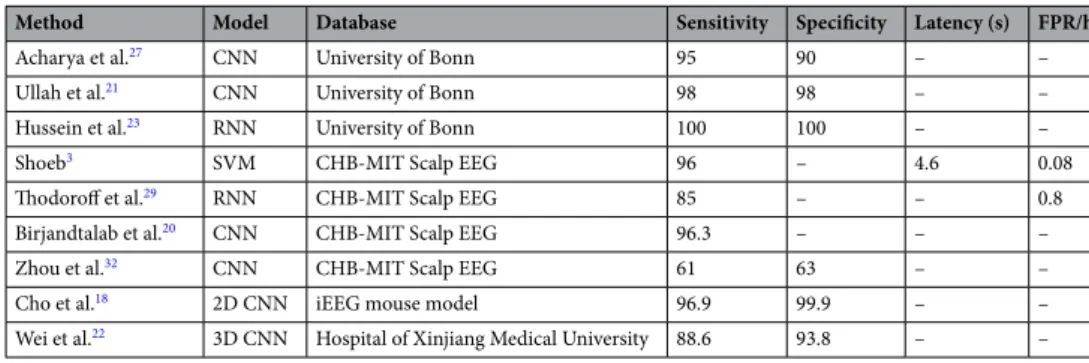
are summarized in Table 1. In this table, the first two columns refer to the method, the third to the database used for the evaluation, and the last ones to the reported metrics, when available, for evaluating the algorithm: classification and sensitivity in the range [0, 100], latency in seconds and false positive rate per hour (FPR/h). In the following paragraphs we describe more in detail some of these studies.
Recent contributions to the application of deep learning methods for seizure detection have been developed on the dataset provided by the University of Bonn26. This database allows the study of a variety of tasks since it
comprises intracranial EEG signals of interictal and ictal episodes from epileptic patients, as well as normal scalp recordings of healthy subjects. In particular, in23, a single Recurrent Neural Network (RNN) was proposed to
exploit the temporal dependencies in EEG signals, which was evaluated in a binary (normal EEG vs. ictal) and a multi-class classification (normal vs. interictal vs. ictal) schemes. In27, a 13-layer Convolutional Neural Network
(CNN) was evaluated on a variant of the multi-class problem, which directly included the pre-ictal category. In the binary task, the authors of21 defined an augmentation scheme with overlapping windows to alleviate the few
available data to train deep learning models. In addition, they introduced a pyramidal one-dimensional CNN that leverages local information to generate a final prediction. Although the previous methods successfully detected seizures segments, they require additional adjustments to process multi-channel data, and more importantly, they need to be validated on long-term EEG signals since the very short duration of recordings in this database (23.6s) prevents an evaluation of their robustness and generalization capabilities.
In parallel to the Bonn dataset, several other studies tested their algorithms for seizure detection using the CHB-MIT Scalp EEG database3,28. The advantage of this collection of signals is that it contains continuous
long-term recordings that can last several hours, which, combined with detailed clinical annotations about seizures times, makes it very suitable for comparisons between different methods. In particular, in29, the authors proposed
a deep learning approach in a supervised learning framework to automatically learn more robust features. They used a RNN architecture in a leave-one-out scheme that captures spectral, spatial and temporal patterns repre-senting a seizure. In addition, a novel input representation was proposed in which an image representation of EEG signals was created combining spatial information (electrodes montage) with the magnitude of different frequency bands as the pixel attribute. In20, a CNN model based on multilayer perceptrons was proposed in
which time domain signals were transformed to frequency domain features by calculating the power spectrum density for 10-s windows. In addition to Sensitivity, they report more reliable metrics, such as Precision and F-measure, obtaining a performance of around 95% for this last one. Nevertheless, the authors chose only 8 h of known non-seizure data for each patient, which does not correspond to the actual class imbalance present in the database. In a similar approach30, EEG signals were transformed to power spectrum density energy diagrams
which are fed into a deep CNN in a transfer learning strategy to classify four categories of epileptic states. Using a subset of 11 patients and only 116 min for the inter-ictal and pre-ictal classes from this dataset, they obtained an average classification accuracy of 90% for seizure episodes. Alternatively, using raw EEG signals in the time domain, the authors in31 trained a CNN model to detect inter-ictal epileptic discharges as well as seizure onsets.
Table 1. Performance comparison of recent seizure detection studies with automated models.
Method Model Database Sensitivity Specificity Latency (s) FPR/h
Acharya et al.27 CNN University of Bonn 95 90 – –
Ullah et al.21 CNN University of Bonn 98 98 – –
Hussein et al.23 RNN University of Bonn 100 100 – –
Shoeb3 SVM CHB-MIT Scalp EEG 96 – 4.6 0.08
Thodoroff et al.29 RNN CHB-MIT Scalp EEG 85 – – 0.8
Birjandtalab et al.20 CNN CHB-MIT Scalp EEG 96.3 – – –
Zhou et al.32 CNN CHB-MIT Scalp EEG 61 63 – –
Cho et al.18 2D CNN iEEG mouse model 96.9 99.9 – –
They obtained an overall seizure detection sensitivity of around 90% but, as in other studies, only a subsample of all available data limited to few hours was used to train and evaluate their model. In another study32, the authors
employed a CNN to compare the seizure detection performance from time and frequency domains through the use of raw signals and their corresponding spectral representation respectively. In addition to scalp EEGs, the algorithms were also tested in intracranial recordings from a different dataset. Surprisingly, while they obtained high performances for the frequency domain scheme, the metrics for the time domain strategy in scalp record-ings were very low compared to other approaches (see Table 1).
Using different datasets, other approaches have evaluated alternative input modalities for CNNs in seizure detection. For instance, in18, in addition to 5-s raw time-series as input, the authors explored a transformed black
and white image of the raw waveforms, a periodogram between 0 and 99 Hz, and a gray scale image of the short-time Fourier transform. These data representations were extracted from intracranial EEGs (single channel) from a mouse model of epilepsy, and further validated on a human intracranial EEG dataset. For each input modality, different architectures were evaluated depending on the dimensionality of the data (1D or 2D). In another study, the authors proposed the use of 3D inputs from multi-channel EEG recordings22; the results over 13 patients
with 159 seizures demonstrated that 3D models surpassed 2D models in metrics such as accuracy, specificity and sensitivity in about two points. However, 3D models have a larger number of parameters to be learned, and thus require much more training samples. An alternative to reduce the number of parameters was proposed in19
using Fully Convolutional Networks (FCN) for neonatal seizure detection. The FCN architecture had a Global Average Pooling layers that replaced the fully connected ones. The experiments were conducted on a large dataset of continuous multi-channel neonatal EEG totaling 834 h and 1389 seizures from 18 newborns, and tested on a public dataset of neonatal EEG waveforms collected at Helsinki University Hospital. The area under the receiver-operating curve (AUC) for specificities over 90% was 86.9% for the 18 test patients.
In this work, we address the seizure detection problem following a deep learning strategy derived from robust methods for object recognition tasks in the computer vision field. Our intention is to mimic the visual inspec-tion performed by clinical specialists when reading EEG recordings. For this, we propose a strategy to generate image representations of raw EEG signals that we use as inputs to our seizure detection algorithms. We tested our strategies in two different datasets, one with only scalp electrodes and the other with combined scalp and intracranial recordings. Our lightweight model with only 314 thousand parameters and minimal pre-processing steps reached high seizure detection performance, comparable or even improving previous studies in which signal transformations are needed for its implementation. Furthermore, in addition to the evaluation on a standard database for seizure detection, we had the special opportunity to compared our seizure detection algorithm on scalp and intracranial recordings in the same subject and to evaluate transfer learning strategies between these modalities, as we have simultaneous signals from the EPILEPSIAE dataset.
Results
CHB‑MIT Scalp EEG.
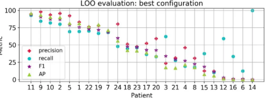
In order to choose the best architecture for our detection model, we explored several configurations of Fully Convolutional Networks (FCN) in the 3-Fold Cross Validation (3FCV) setup (see the Methods section and Table 2 in the supplementary material), and with the best configuration, we trained and evaluated the Leave-One-Patient-Out (LOO) model to evaluate the model’s capacity to detect seizures on data from unseen patients. The best model configuration is a FCN with 3 blocks, 128 filters, and dropout layers with probabilities of 0.1 and 0.3 at the early and last convolutional layers, respectively. We included a L2 regulariza-tion (weight decay) that helps the network to generalize better. The results are summarized in Fig. 1 (left bar graphs). For all patients, we obtained global accuracy and specificity levels of 92.9 ± 21.8 (MEAN ± STD) and 93.1 ± 21.9 , respectively. In addition, we reached global values for precision of 51.4 ± 34.1 , recall of 53.1 ± 25.5 , F-measure of 46.6 ± 31.0 and the AP 44.4 ± 34.4.Individual metrics per patient are presented in Fig. 2. Overall, 33% of the patients reached a F-measure greater than 70% (n = 255 recordings), 20% obtained a precision over 90% (n = 153 recordings) and another 20% a
Figure 1. Average metrics for the LOO and First Seizures models evaluated in the CHB-MIT Scalp EEG
database. Each color bar corresponds to a different metric, with the average value at the bottom and the standard error of the mean ( σ/√N ) as blue lines.
recall over 80% (n = 140 recordings). When we contrasted the performance with the number of seizures per patient, we noticed that the metrics tended to decrease with an increasing number of seizures, whereas patients with less seizures have both high precision and recall values (see for instance patients 11, 9 and 2). Qualitative results of accurate detections and limitations are shown in Fig. 3. In this figure, we provide an example of an accurate match between the annotated and detected seizure times (Fig. 3A); an example of long-term accurate detections in more than 25 h of recording (the ground truth lines are covered by the detections in red, Fig. 3B), and a segment with false positives and disrupted detections (Fig. 3C).
Based on the results obtained individually, we identified some patients as difficult, with seizures harder to detect than others. Thus, in order to exploit the model’s capacity to learn from hard seizure instances, and there-fore to increase the performance for challenging patients, we proposed to train another cross-patient model with data from the first 80% of recordings with seizures and evaluate in the remaining ones, referred as First Seizures model in Fig. 1. Compared to the performance in the best LOO model, the average accuracy and specificity were notably higher for First Seizures setup, reaching values of 99.3 ± 1.16 and 99.6 ± 0.59 , respectively. In addition, the precision ( 62.7 ± 30.2 ), F-measure ( 59.0 ± 25.9 ) and AP ( 54.5 ± 31.5 ) for the First Seizures strategy improved in more than 10 points while the recall increased by 5 points ( 58.3 ± 22.9 ). Furthermore, we obtained a noticeable improvement for patients with seizures hard to detect. For instance, for patient 12 the precision increased from
Figure 2. Results for the LOO model with the best configuration. Patients in the x-axis are sorted by decreasing
F-measure (purple star marker).
Figure 3. Qualitative results for the best LOO model (base FCN + DO). Annotations (blue) and predictions
1.55 (in the LOO model) to 48.1, while keeping almost the same recall (60%). For each patient, the performance in the First Seizures model is presented in Fig. 4. For a comparison of the performance of individual patients under the three different cross-patient models see Table 3 in the supplementary material.
For the LOO and First Seizures models, we calculated the false positive rate (FPR) as in33. In particular, we
defined the false alarm rate as the number of false alarms per hour of recording. To count the false alarms in the predictions, we analyzed consecutive 30-s segments of signal, as defined in29. First, we changed from class
probabilities to binary predictions using a threshold corresponding to the best F-measure, and then, following the standard evaluation for object detection34, if more than the 50% of the window was predicted as the seizure
class, the window was compared to the corresponding time segment in the annotations. Figure 5 presents the FPR/h for all patients individually and for both model configurations. In the LOO model, the average FPR/h was 7.80 ± 26.1 ranging from 0 to 119.9. Even though the false alarm rate was distributed within a wide range, 83% of the patients obtained a rate below 0.5 false alarms per hour, with an average FPR/h for the values within the 95% percentile equal to 0.39 ± 1.15 . The FPR/h range for all patients decreased considerably in the First Seizures model, [0–2.14], with an average of 0.14 ± 0.45.
EPILEPSIAE.
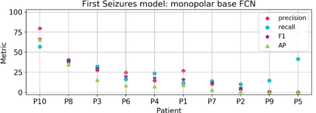
To compare the results between the EPILEPSIAE and CHB-MIT Scalp datasets, we first carried out experiments using only scalp electrodes from the former database in the First Seizures setup. We departed from the parameter exploration conducted in the CHB-MIT dataset and used the base FCN with Dropout (DO) and weight decay. For this model configuration, we explored a finetuning strategy using the First Seizures model in CHB-MIT patients as the weight initialization. Besides, we evaluated models trained from scratch with electrodes in monopolar and bipolar configuration. For a complete comparison of the experiments in EPILEPSIAE patients with scalp recordings refer to Fig. 1 in the Supplementary Material. We summarize the best results achieved with the monopolar model in Fig. 6. Among all patients, we obtained an average F-measure of 20.8 ± 19.1 , an AP of 14.7 ± 19.6 , a recall of 25.9 ± 14.9 and a precision of 22.9 ± 22.8 . Overall, these met-rics showed a strong variation among patients, and a low performance for 8 out of 10, which is reflected in the reduced average performance. However, the average accuracy of 98.0 ± 3.34 and specificity of 98.3 ± 3.4 are not affected because of the large amount of true negatives. In addition, we calculated the number of false alarms per hour obtaining an average among the 10 patients of 1.20 ± 2.66 (ranging from 0.0 to 9.08 FPR/h).For demonstrative purposes, we visualized the predictions of the models for three chosen patients, as shown in Fig. 7. Here, Fig. 7A corresponds to an example of two seizures that were correctly detected; Fig. 7B presents a false positive detection and a short seizure that is not well delimited; finally, Fig. 7C provides an example of a
Figure 4. Results of the First Seizures model for all patients. Patients in x-axis are sorted by decreasing
F-measure.
Figure 5. False positive rate per hour defined in consecutive 10s windows for the best LOO model (blue) and
First Seizures model (red). Patients are sorted by increasing FPR/h. The y-axis is cut at FPR/h value of 0.5 to visualize minor differences. Patients 15, 16, 12 and 14 have values over 2 and are not shown in the plot.
patient with noisy recordings. This kind of segments could explain a reduced ability for the model to identify seizures, and thus, the reduced overall performance.
Intracranial electrodes. With the objective to evaluate the contribution of invasive recordings to our seizure
detection algorithm, we included the intracranial electrodes information in addition to the scalp ones. For this, we trained patient-specific models since the locations of implanted contacts were unique to each patient. We selected the patients with the highest number of seizures (at least 9), giving us four patients in total (P3, P6, P8 and P10). Examples of ictal and inter-ictal instances are shown in Fig. 8. To determine the best model for each patient, we explored different configurations between monopolar and bipolar intracranial and/or scalp elec-trodes as input. Besides, we initialized each patient-specific model with the best model found with scalp record-ings from all the EPILEPSIAE patients as a transfer learning strategy.
The results with the best model obtained for each patient are summarized in Table 2 (for a complete com-parison between experiments with intracranial data refer to Table 4in the supplementary material). Patient P3
Figure 6. Average metrics for the best experiment in EPILEPSIAE patients using scalp electrodes only. Patients
in the x-axis are sorted by decreasing F-measure (purple star marker).
Figure 7. Qualitative results in the evaluation recordings of the best scalp model in the EPILEPSIAE patients.
The y-axis shows the monopolar electrodes, and the x-axis the time in seconds. Blue lines correspond to annotations, and red lines to predictions.
is not displayed because neither model could learn to detect seizures in its recordings. For P8, we identified that training models only with intracranial electrodes (denoted as intra) improved all the metrics compared to the scalp-only models. For this patient, the results further improved when we finetuned the cross-patient monopolar scalp model to the patient-specific monopolar intracranial model (Monopolar-intra-FT in Table 2). We visual-ized one of these seizures in Fig. 9; here, it is possible to observe that our detection (red lines) is disrupted at the beginning of the seizure, when ictal patterns are not as evident as in the subsequent seconds, but the seizure
Figure 8. Signal representation of intracranial electrodes in monopolar configuration (57 intracranial contacts
for P10). The y-axis corresponds to the intracranial channels labeled as iEN and the x-axis to the temporal
dimension. Top and bottom rows present examples of ictal and interictal periods, respectively.
Table 2. Evaluation metrics using the First Seizures configuration with intracranial data from three patients of
the EPILEPSIAE database.
First seizures with intracranial electrodes
Patient Best model Acc. Spec. Prec. Rec. F1 AP
P8 Monopolarintra FT 99.6 83.1 94.9 82.8 88.4 90.3 P10 Bipolarboth zero 99.9 83.6 97.6 83.5 90.0 89.3 P6 Monopolarboth zero 99.5 8.12 12.7 7.82 9.68 3.04 Mean ± std – 99.7 ± 0.17 58.3 ± 35.5 68.4 ± 39.4 58.0 ± 35.5 62.7 ± 37.5 60.9 ± 40.9
Figure 9. Detections in the evaluation recordings of P8 with the monopolar-intracranial-finetuning setup. The
y-axis shows the intracranial electrodes in monopolar configuration, and the x-axis the time in seconds. Blue lines correspond to annotations and red lines to predictions.
end is accurately identified. For P10 and P6 patients, the combination of both electrode types further improved the results in the bipolar and monopolar configurations respectively, even though most of the metrics for P6 remained deficient. Consistently, patient-specific models trained from scratch only with scalp electrodes in a bipolar configuration (Bipolar-scalp-zero in Table 4 from the supplementary materia) reached similar results to those reported in the cross-patient model (Figure 1 in the Supplementary material) for P8 and P10.
Discussion
In this work, we have explored and validated state-of-the-art strategies based on deep learning approaches for the automatic detection of epileptic seizures. The main advantage of our method is that it does not need any estimation of pre-selected features for their execution, which usually requires the intervention of trained techni-cians or engineers, thus limiting their use to restricted environments. Besides, our method requires minimum pre-processing stages from raw EEG signal, i.e. signal saturation at ± 250 µ V to reduce noise, avoiding filtering and domain transformations. Our algorithms tested in hundreds of hours of scalp and intracranial recordings evidenced high performances on the usual metrics of accuracy and sensitivity, which are comparable or even higher than those reported in previous works. In addition, due to the large class imbalance between ictal and inter-ictal episodes, we report more appropriate metrics such as the precision, the F-measure, the AP, and recall, for which we reached high results for some of the analyzed patients.
The comparison of our results with previous studies is not straightforward since there is not a standard evalu-ation for the seizure detection problem; each author reports its own metrics and the definition of a positive or negative sample depends on the window length being analyzed. To provide the possibility to fully reproduce our results and allow future comparisons, we make publicly available our source code and trained models in GitHub. Despite this, we still compared our method with the metrics of a recent report in the CHB-MIT dataset32. In this
work, the authors trained and evaluated their algorithm for each patient individually, but they did not specify how data was split into train and test sets. Comparing the average accuracy and specificity of our best model in the First Seizures configuration ( 99.3 ± 1.16 and 99.6 ± 0.59 respectively), we obtained a performance that is superior to the one reported by the authors in the inter-ictal vs. ictal task (accuracy of 62.3 and specificity of 63.3), but their recall (61.2) was greater by 3 points. However, as mentioned above, due to the large class imbal-ance of ictal to inter-ictal episodes, the accuracy and specificity might be presented in conjunction with more robust metrics to imbalance tasks, such as the precision or the FPR/h.
In another recent work using the same CHB-MIT Scalp EEG database29, the average recall or sensitivity was
85% for cross-patients models in a LOO configuration, but the authors do not report precision. Instead, they computed the false positive rate per hour (0.8/h) for their predictions over every 30-s segment of the signal. In our evaluation of false positives in 30-s windows, the average FPR/h of 7.81 is inflated by the low performance of 4 patients (6, 12, 14 and 16), which also affected the precision and recall metrics. Considering only the FPR/h values within the 95% percentile, our average rate 0.39/h is half the one reported in29. To compare the performance for
each patient, the authors presented graphs with individual metrics as the difference of their performance with a previous approach35, making the comparison difficult. Despite this, we agreed on the performance of patients
with the most challenging seizures to detect, such as 6, 12 and 16.
In order to improve the detection performance and to provide the model with better capabilities for gener-alization, we included prior information from the recordings in the First Seizures setup. Since the model has already seen seizure samples from all patients, all the average metrics increased. In particular, while the metrics for the patients identified as hard in the LOO setup improved, the performance of the easy patients remained almost unchanged. In addition, under the First Seizures configuration, the FPR/h was zero for 18 out of the 24 patients, meaning that there are no false positives in the predictions.
In the models with EPILEPIAE patients, we observed that finetuning from models that have already been trained to identify ictal from inter-ictal activity in a bipolar configuration of electrodes did not improve the results as expected. The metrics were similar when models were trained from scratch. Even so, our model achieved high accuracy and specificity values close to 100% ( 98.0 ± 3.34 and 98.3 ± 3.40 respectively). However, the other metrics were considerably low, having average values over 25%. This disparity can be explained by the robustness of each metric to imbalanced data. When we included the intracranial channels, we found an improvement of seizure detection in two patients (P8 and P10), for whom the models with scalp data had satisfactory results. We also found a slight gain in performance for the other two patients, but overall, the algorithm failed to detect seizures in the recordings from these patients, as demonstrated in the experiment using only scalp electrodes. We attribute the improvement of including intracranial electrodes to the better spatial localization, and less artifacts than those present in scalp EEG36. In addition, seizure patterns may emerge stronger over specific electrodes
according to the origin of the seizure activity. For a better validation of the contribution of intracranial electrodes to the seizure detection problem, we must test these configurations in a more representative group of patients.
In conclusion, the large variability in the evaluation metrics for different patients reflects the difficulty of the problem, and the challenges in defining a cross-patient model that can generalize well for patients that it has never seen before. Cross-patient models can be improved if the model learns from instances that include the first recorded seizures. Finally, the inclusion of intracranial channels in addition to the scalp ones in a patient-specific model improved all metrics for some patients, suggesting that both types of recordings carry complementary information that is needed for a better detection of epileptic seizures.
Methods
Dataset description.
CHB‑MIT scalp EEG database. This epilepsy dataset consists of scalp EEG signalsfrom 23 pediatric subjects with intractable seizures admitted at the Boston Children’s Hospital3, which is publicly
elec-trode positioning in bipolar configuration, sampled at 256 Hz with 16-bit depth. Each recording was annotated by experts indicating seizure beginning and ending times in seconds. From the 24 cases, we analyzed a total of 941.6 h of inter-ictal activity and 3 h of ictal acitivity from 181 annotated seizures (see Table 1 in the supplemen-tary materia for a complete description of cases).
EPILEPSIAE. The European Epilepsy Database contains high-quality EEG recordings of 275 epilepsy
patients37. Raw EEG data comprise at least 5 days of continuous recording for each subject, with several scalp
and/or intracranial channels. The dataset contains metadata information about recordings and patients, includ-ing the EEG onset and offset times for all of the seizures (in a date-hour format), the electrodes involved in the seizure activity (primary and secondary propagations), additional classification of the seizures, among others, all annotated by specialist neurologists. From the 275 patients, only 50 have intracranial recordings, and 225 have additional scalp EEG. Intracranial channels consisted of implanted grids, strips and/or depth electrodes, with a variable number of invasise contacts depending on each patient. Surface recordings consisted of 10-20 or 10-10 standard EEG electrode placement. From these patients, we selected the ones that fulfilled the requirement of simultaneously having intracranial and scalp recordings (n = 10 patients), the latter with the same channels of the CHB-MIT patients for comparison purposes. All signals were originally sampled at 1024 Hz with a 16-bit resolution and then downsampled to 256 Hz for the analyses. From this database, we analyzed a total of 1302.2 h of inter-ictal activity, and 2.5 h of ictal activity from 109 annotated seizures (see Table 1 in the Supplementary material for a complete description). Seizures segments shorter than 9s were discarded.
Data representation.
Signal representation. To change from signals to images domain, we took the rawamplitude at each sample and channel as the pixel attribute of a 2D image, where the rows corresponded to the different EEG channels aligned vertically, and the columns to the temporal dimension. For the CHB-MIT dataset, we standardized the order of electrodes across all patients by choosing the 23 common bipolar channels among all the registers. We then split the time course of EEG signals into segments (windows) of 4-s of duration, so each resulting image had dimensions of N × (4 × SamplingRate) , where N is the number of channels (re-corded electrodes), and SamplingRate the number of samples per second depending on the dataset. We wanted to design seizure detection methods requiring a minimum of pre-processing steps, as these last require several subjective considerations that we wanted to avoid. For this and intending to reduce the more prominent artifacts, we saturated the scalp EEG signals with a threshold amplitude of ± 250 µ V and used the raw amplitudes without any further pre-processing.
Different examples of the obtained images for ictal and inter-ictal instances are shown in Fig. 10. In this fig-ure, the amplitude of each time point is encoded through a grey scale. This visualization offers the posibility to determine changes in the spatial and temporal dimensions during an ictal and inter-ictal period, and to identify the electrodes that are mostly involved in a seizure.
Data augmentation. Data augmentation is crucial to avoid overfitting in Neural Networks38. Previous
studies8,21 have defined augmentation strategies to train CNN using additional examples defined by overlapping
temporal windows with small shifts. Due to the spontaneous nature of epileptic seizures and their short duration compared to the extensive recording of inter-ictal activity, we augmented the number of training examples for the ictal class. To do so, we created overlapped images during the complete seizure duration with a time-shift between consecutive windows of 1/8 and 1/16 s for the CHB-MIT and EPILEPSIAE datasets, respectively. Even after data augmentation, the class imbalance remained. Thus, the inter-ictal instances were then randomly
sub-Figure 10. Examples of the signal representation taking the amplitude as the pixel attribute for four patients
from the CHB-MIT Scalp dataset. The height encodes the channels in bipolar configuration, and the width the window length (4 s) with the aspect ratio adjusted for visualization purpose. The colorbar displays the amplitude range of the signals in µ V. Top row: ictal examples, bottom row: interictal examples.
sampled such that a fraction of them was close to the seizures, by defining a temporal closeness parameter as 150s before and after, and the other fraction was sampled far from the seizures. The inter-ictal instances close to the seizures were augmented with the same strategy mentioned before, but with a time-shift between con-secutive windows of 1/4 and 1/8 s for the CHB-MIT and EPILEPSIAE datasets, respectively. No overalapping between consecutive windows was used for inter-ictal instances far from the seizures.
Detection algorithm.
Fully convolutional networks (FCN). Convolutional Neural Networks have beenused to address object recognition tasks due to their ability to encode the input in multiple representations on its hidden layers, and propagate it through the network to produce an output with a final classification stage that is usually a fully connected layer. To make dense predictions for per-pixels tasks, CNN changed to FCN by replacing fully connected layers with convolutional layers, with kernels of the same dimension as the input39. The
advantage of using FCNs is that they produce dense outputs from arbitrary-sized inputs, thus, they are able to process recordings of different lengths. For our classification problem, the inputs of the networks corresponded to the raw EEG matrix images, which were split in two classes: ictal and interictal (positive and negative classes respectively).
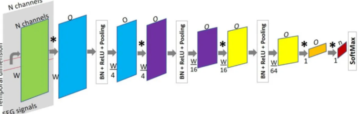
For classifying neural activity states we designed a base FCN network with 3 blocks. Each block consisted of convolution, Batch Normalization, non-linear transformation ReLU, and Pooling layers, followed by two fully convolutional layers and a final SoftMax layer, as shown in Fig. 11. The purpose of the SoftMax layer was to rescale the elements from the output of the last convolutional layer in the range (0, 1), such that the final output of the network was a probability vector of either class.
Initially, the number of input channels for the convolutional layers corresponded to the same channels of the recordings, and then, the channel dimension denoted the number of features learned at each convolutional layer. The dimensionality of the input was reduced only along the temporal axis in each pooling layer. The kernels in the last convolutional layers, which replace the fully connected ones, were defined such that the network produced a class label every window of a fixed size. In this way, the input could be of variable length and the number of predictions depended on the length of the input (recording) to be evaluated.
We further introduced two regularization strategies for Deep Neural Networks. The first one, referred as Dropout (DO), prevents that the units of the model from co-adapting to the training data by randomly drop-ping out units and their connections40. The second one, L2 regularization (weight decay) helps the network to
generalize better.
Due to the limited number of patients, seizures and their short duration, we used a transfer learning strategy, called finetuning, to train a model in a database that does not have sufficient size41. In brief, once a model has
been trained on a base dataset for a specific task, the learned features are transferred to a second network that is trained with samples from a different dataset for a new task. The weights of the pretrained model are said to be finetuned by continuing backpropagation. All the layers from the network can be finetuned, or only a fraction by freezing the weights of the layers that want to be preserved. This process will work if the learned features could be generalized, and if the nature of both the tasks and data is similar.
Models and evaluation.
CHB‑MIT Scalp EEG. In the CHB-MIT Scalp EEG dataset, we definedcross-patient models by splitting the recordings from the cross-patients in two ways. First, in the 3 fold Cross-Validation (3FCV), we divided patients into three sets by training in two sets and evaluating in the remaining one, such that we covered the three possible combinations. Second, in the Leave‑One‑Patient‑Out (LOO), 24 models were trained, each one using data from k − 1 patients (where k is the total number of patients), and evaluated in all the recordings of the patient left out. In both configurations, we sampled 4s windows of the ictal and inter-ictal classes from the recordings of the patients in the train set, and evaluated our model in the complete recordings of the patients in the test set.
Figure 11. Proposed FCN architecture for the automated classification of EEG recordings into ictal and
interictal states. The temporal dimension is reduced by 4 × at every block (blue, purple and yellow). *A convolution operation, n is the number of classes, W is the window width, and O is the number of output channels in the respective convolutional layer.
exploration conducted in the CHB-MIT dataset and used the base FCN architecture with DO and weight decay. First, we finetuned the best model in CHB-MIT patients to detect seizures on EPILEPSIAE patients. To do so, we adjusted the scalp electrodes in the same bipolar configuration, and initialize the weights of the new model with the pre-trained ones. The complete weights of the new model were optimized in the training partition for EPILEPSIAE patients. Alternatively, we trained models from scratch with ictal and inter-ictal examples from EPILEPSIAE patients, changing the electrode configuration (monopolar) and the number of filters in the con-volutional layers.
To include the information from the intracranial electrodes, we trained patient-specific models in the first seizures model setup. The three strategies to train the models were: (i) training from scratch using only scalp or intracranial electrodes, and their combination, (ii) the models from (i) in a monopolar and bipolar configuration, and (iii) finetuning of a model pretrained in the first recordings with seizures of the 10 EPILEPSIAE patients, adapting the input size to the number of intracranial channels only. Given that the preexisting models were trained in scalp recordings, we included an initial convolutional layer that mapped from N intracranial channels to the number of scalp electrodes. The parameters for this new layer were learned during the training phase. The bipolar montage for the intracranial channels was defined differently for each patient as the difference between adjacent electrodes of the same electrode bundle, following the same strategy as in43.
Evaluation metrics. We evaluated the performance of the algorithms using the standard metrics of seizure
detection problems4: accuracy ((true positives+true negatives)/(positives+negatives)), specificity (true
nega-tives/(true negatives+false positives)) and sensitivity (true posinega-tives/(true positives+false negatives)), and also included those of detection problems: precision (true positives/(true positives+false positives)), recall or sen-sitivity, F-measure (harmonic mean of precision and recall), also called F1 score, and Average Precision (AP), which is defined as the area under the precision-recall (PR) curve built with different confidence thresholds according to the probability of belonging to the ictal class. The global performance of a model was given by the average ± standard deviation of the metrics across all patients in a given evaluation set.
Received: 11 September 2020; Accepted: 26 November 2020
References
1. Ferreira, J. & Mestre, T. Eslicarbazepine acetate: A new option for the treatment of focal epilepsy. Expert Opin. Investig. Drugs 18, 221–229 (2009).
2. Tzallas, A. T. et al. Automated epileptic seizure detection methods: a review study. In Epilepsy‑histological, electroencephalographic and psychological aspects (InTech, 2012).
3. Shoeb, A. H. & Guttag, J. V. Application of machine learning to epileptic seizure detection. In Proceedings of the 27th International Conference on Machine Learning (ICML‑10), 975–982 (2010).
4. Siddiqui, M. K., Morales-Menendez, R., Huang, X. & Hussain, N. A review of epileptic seizure detection using machine learning classifiers. Brain Inform. 7, 1–18 (2020).
5. Paul, Y. Various epileptic seizure detection techniques using biomedical signals: a review. Brain Inform. 5, 6 (2018).
6. Hussein, R., Palangi, H., Ward, R. & Wang, Z. J. Epileptic seizure detection: A deep learning approach. arXiv preprintarXiv :1803.09848 (2018).
7. Cecotti, H. & Graser, A. Convolutional neural networks for p300 detection with application to brain-computer interfaces. IEEE Trans. Pattern Anal. Mach. Intell. 33, 433–445 (2010).
8. Kwak, N.-S., Müller, K.-R. & Lee, S.-W. A convolutional neural network for steady state visual evoked potential classification under ambulatory environment. PLoS ONE 12, e0172578 (2017).
9. Thomas, J., Maszczyk, T., Sinha, N., Kluge, T. & Dauwels, J. Deep learning-based classification for brain-computer interfaces. In 2017 IEEE International Conference on Systems, Man, and Cybernetics (SMC), 234–239 (IEEE, 2017).
10. Nagel, S. & Spüler, M. World’s fastest brain-computer interface: Combining eeg2code with deep learning. PLoS ONE 14, e0221909 (2019).
11. Yildirim, O., Baloglu, U. B. & Acharya, U. R. A deep learning model for automated sleep stages classification using PSG signals. Int. J. Environ. Res. Public Health 16, 599 (2019).
12. Supratak, A., Dong, H., Wu, C. & Guo, Y. Deepsleepnet: A model for automatic sleep stage scoring based on raw single-channel EEG. IEEE Trans. Neural Syst. Rehabil. Eng. 25, 1998–2008 (2017).
13. Mousavi, S., Afghah, F. & Acharya, U. R. Sleepeegnet: Automated sleep stage scoring with sequence to sequence deep learning approach. PLoS ONE 14, e0216456 (2019).
14. Michielli, N., Acharya, U. R. & Molinari, F. Cascaded LSTM recurrent neural network for automated sleep stage classification using single-channel EEG signals. Comput. Biol. Med. 106, 71–81 (2019).
15. Tsiouris, K. M. et al. A long short-term memory deep learning network for the prediction of epileptic seizures using EEG signals. Comput. Biol. Med. 99, 24–37 (2018).
16. Khan, H., Marcuse, L., Fields, M., Swann, K. & Yener, B. Focal onset seizure prediction using convolutional networks. IEEE Trans. Biomed. Eng. 65, 2109–2118 (2018).
17. Liang, J., Lu, R., Zhang, C. & Wang, F. Predicting seizures from electroencephalography recordings: A knowledge transfer strategy. In 2016 IEEE International Conference on Healthcare Informatics (ICHI), 184–191 (2016).
18. Cho, K.-O. & Jang, H.-J. Comparison of different input modalities and network structures for deep learning-based seizure detec-tion. Sci. Rep. 10, 1–11 (2020).
19. O’Shea, A., Lightbody, G., Boylan, G. & Temko, A. Neonatal seizure detection from raw multi-channel EEG using a fully convo-lutional architecture. Neural Netw. 123, 12–25 (2020).
20. Birjandtalab, J., Heydarzadeh, M. & Nourani, M. Automated EEG-based epileptic seizure detection using deep neural networks. In 2017 IEEE International Conference on Healthcare Informatics (ICHI), 552–555 (IEEE, 2017).
21. Ullah, I. et al. An automated system for epilepsy detection using EEG brain signals based on deep learning approach. Expert Syst. Appl. 107, 61–71 (2018).
22. Wei, X., Zhou, L., Chen, Z., Zhang, L. & Zhou, Y. Automatic seizure detection using three-dimensional CNN based on multi-channel EEG. BMC Med. Inform. Decis. Mak. 18, 111 (2018).
23. Hussein, R., Palangi, H., Ward, R. K. & Wang, Z. J. Optimized deep neural network architecture for robust detection of epileptic seizures using EEG signals. Clin. Neurophysiol. 130, 25–37 (2019).
24. Goodfellow, I., Bengio, Y. & Courville, A. Deep Learning (MIT Press, Cambridge, 2016).
25. Russakovsky, O. et al. Imagenet large scale visual recognition challenge. Int. J. Comput. Vis. 115, 211–252 (2015).
26. Andrzejak, R. G. et al. Indications of nonlinear deterministic and finite-dimensional structures in time series of brain electrical activity: Dependence on recording region and brain state. Phys. Rev. E 64, 375 (2001).
27. Acharya, U. R., Oh, S. L., Hagiwara, Y., Tan, J. H. & Adeli, H. Deep convolutional neural network for the automated detection and diagnosis of seizure using EEG signals. Comput. Biol. Med. 100, 270–278 (2018).
28. Goldberger, A. L. et al. Physiobank, physiotoolkit, and physionet: Components of a new research resource for complex physiologic signals. Circulation 101, e215–e220 (2000).
29. Thodoroff, P., Pineau, J. & Lim, A. Learning robust features using deep learning for automatic seizure detection. CoRR (2016). arXiv :1608.00220 .
30. Gao, Y., Gao, B., Chen, Q., Liu, J. & Zhang, Y. Deep convolutional neural network-based epileptic electroencephalogram (EEG) signal classification. Front. Neurol. 11, 375 (2020).
31. Wei, Z., Zou, J., Zhang, J. & Xu, J. Automatic epileptic EEG detection using convolutional neural network with improvements in time-domain. Biomed. Signal Process. Control 53, 101551 (2019).
32. Zhou, M. et al. Epileptic seizure detection based on EEG signals and CNN. Front. Neuroinform. 12, 95 (2018).
33. Beniczky, S. & Ryvlin, P. Standards for testing and clinical validation of seizure detection devices. Epilepsia 59, 9–13 (2018). 34. Girshick, R. Fast r-cnn. Proceedings of the IEEE International Conference on Computer Vision 1440–1448 (2015).
35. Wilson, S. B., Scheuer, M. L., Emerson, R. G. & Gabor, A. J. Seizure detection: Evaluation of the reveal algorithm. Clin. Neurophysiol.
115, 2280–2291 (2004).
36. Buzsaki, G. Rhythms of the Brain (Oxford University Press, Oxford, 2006).
37. Klatt, J. et al. The epilepsiae database: An extensive electroencephalography database of epilepsy patients. Epilepsia 53, 1669–1676 (2012).
38. Krizhevsky, A., Sutskever, I. & Hinton, G. E. Imagenet classification with deep convolutional neural networks. Adv. Neural Inf. Process. Syst. 66, 1097–1105 (2012).
39. Long, J., Shelhamer, E. & Darrell, T. Fully convolutional networks for semantic segmentation. CoRR (2014). arXiv :1411.4038. 40. Srivastava, N., Hinton, G., Krizhevsky, A., Sutskever, I. & Salakhutdinov, R. Dropout: A simple way to prevent neural networks
from overfitting. J. Mach. Learn. Res. 15, 1929–1958 (2014).
41. Yosinski, J., Clune, J., Bengio, Y. & Lipson, H. How transferable are features in deep neural networks? CoRR (2014). arXiv :1411.1792. 42. Mirowski, P. W., LeCun, Y., Madhavan, D. & Kuzniecky, R. Comparing svm and convolutional networks for epileptic seizure pre-diction from intracranial eeg. In IEEE Workshop on Machine Learning for Signal Processing, 2008 (MLSP 2008), 244–249 (IEEE, 2008).
43. Klimes, P. et al. The functional organization of human epileptic hippocampus (2016).
Author contributions
Study design: C.G., P.A., M.V. Data collection and preparation: M.L.v.Q., C.A., M.N., M.V. Data Analysis and interpretation: C.G., P.A., M.V. Writing of manuscript: C.G., P.A., M.N., C.A., M.L.v.Q, M.V.
Competing interests
The authors declare no competing interests.
Additional information
Supplementary Information The online version contains supplementary material available at https ://doi. org/10.1038/s4159 8-020-78784 -3.
Correspondence and requests for materials should be addressed to M.V. Reprints and permissions information is available at www.nature.com/reprints.
Publisher’s note Springer Nature remains neutral with regard to jurisdictional claims in published maps and