The Design of Whispering Gallery Mirrors for Soft X-Ray Lasers
by Tsen-Yu Hung
Submitted to the Department of Electrical Engineering and Computer Science in Partial Fulfillment of the Requirements for the Degree of
Bachelor of Science in Electrical [Computer] Science and Engineering at the Massachusetts Institute of Technology
May 1988 @Tsen-Yu Hung
The author hereby grants to M.I.T. permission to reproduce and to distribute copies of this thesis document in whole or in part.
Author ..
Dep t of Electrical Engineering and Computer Science May 10, 1988
Certified by
AC15iP
Peter L. Hagelstein. Associate Professor Thesis Supervisor Accepted by
Leonard A. Gould Chairman, Department Committee on Undergraduate Theses
JUL 28 1988
08RA FSTHE DESIGN OF WHISPERING GALLERY MIRRORS FOR
SOFT X-RAY LASERS
by Tsen-Yu Hung
Submitted to the Department of Electrical Engineering and Computer Science on May 10, 1988 in partial fulfillment of the requirements for the
degree of Bachelor of Science.
Abstract
Whispering Gallery Mirrors are broad band soft x-ray mirrors that have been demonstrated to achieve close to 70% reflectivity for 180 degree turn, or close to 50% reflectivity for 360 degree turn, which is higher perfonning than other designs, such as the multilayer mirrors. Both the theoretical and experimental aspects of the mirrors are explored in detail.
Literature on the analysis of the electromagnetic field for cylindrical boundary and perfectly conducting and lossy medium is reviewed in detail, from the earliest analysis accomplished by Lord Rayleigh.
Reports on progress made in manipulating the 2D Helmholtz equation for numerical modeling are included. Examinations of both the high frequency limit and the low frequency limit (which correspond physically to x-ray radiation and infrared waveguides, respectively) are described.
Losses of soft x-rays due to scattering is studied by modelling the surface irregularities as Gaussian distribution. Surface smoothness requirements for soft x-rays are described. Losses due to photoabsorption is studied by examining the materials' Cooper Minimum. The term, Cooper Minimum, is briefly explained. Kramer-Kronig analysis is described here and will be used in the near future to compute the optical constants of promising materials for surface coatings.
A survey of the susceptibility to oxidation, toxicity, malleability, and the Cooper Minimum wavelength of the elements Z = 36 - 94 is included. A selection of materials for whispering gallery mirror to reflect light of 200 angstroms wavelength is chosen and described.
Industries who can polish surfaces on the order of tens of angstroms are described. Issues in constructing the whispering gallery mirrors and their solutions are discussed. Techniques to evaluate surface roughness are examined.
Thesis Supervisor: Prof. Peter L. Hagelstein
Title: Associate Professor of Electrical Engineering and Computer Science
Acknowledgements
I express my deepest appreciations to Prof. Peter Hagelstein. His goeing out of his way to satisfy his students' curiosities impresses me. His intellects are beyond brilliance. He, as a mentor, places equal weights in developing his students in both as a scientist and a human being.
I thank Prof. Hank Smith for his caring supports and suggestions.
TABLE OF CONTENTS
I. Introduction
II. Present Status of Whispering Gallery Mirrors
II.1 Lord Rayleigh's Formulation
11.2 Wasylkiwskyj's Formulation
11.3 Ishihara and Felsen's Formulation
II.4 Bahar's Formulation
11.5 Where do we go from here
III. Design Issues of the Whispering Gallery Mirrors
III.A Practical Issues
III.A.2 Glancing angles
III.A.2.1 The size of glancing angle and beam height 33 III.A.2.2 Absorption of soft x-ray in air and one-bounce experiments 33 III.A.2.3 Theoretical problems assoicated with glancing angles 33
III.A.3 Perturbation Analysis of Surface Roughness of the
Whispering Gallery Mirrors 35
III.A.4 Kramers-Kronig Analysis 40
III.A.4.1 Kramers-Kronig's relation 41
III.A.4.2 Utilization of the Cooper Minimum 42
III.A.4.3 Selection of material for our whispering gallery mirror design. 43
Ifl.B Theoretical Design of the Whispering Gallery Mirrors 45
III.B.1 Finite element analysis of 2D Helmholtz equation for an arbitrarily
shaped surface 45
m.B.2 Analysis of 2D Helmholtz for high frequency approximations 50
III.B.3 Analysis of 2D Helmholtz for high low approximations 54
IV. Implementation Issues 57
IV.A Construction of the Whispering Gallery Mirrors Locally 60
IV.A.2 Constructing Whispering Gallery Mirrors
IV.B Surface quality
V. Summary and Conclusion
Appendix A Appendix B Appendix C Appendix D Appendix E References
LIST OF FIGURES
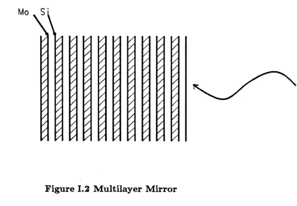
Fig. I.1 Whispering Gallery Mirror Fig. 1.2 Multilayer Mirror
Fig. 1.3 Transmission/reflectivity vs. X-ray energy plot Fig. 1.4 Reflectivity vs. X-ray energy plot
Fig. 1.5 Vinogradov's Data
Fig. II.1.1 Whispering Gallery Mode
Fig. III.A.1 Whispering Gallery Mirror's Focusing Optics Fig. III.A.2.1 Light beam at an interface
Fig. III.A.2.2 Sliding Angle Graph
Fig. IH.A.3.1 Scattering loss vs. Height of surface irregularities Fig. III.A.3.2 Height vs. Correlation radius
Fig. III.A.4.1 Cooper Minima of Ba and La Fig. III.B.1 Arbitrarily shaped surface Fig. IV.B.II.1 CGH
Fig. IV.B.II.2 CGH's viewing arm Fig. IV.B.II.3 CGH fringe patterns Fig. IV.B.II.4 Precision of CGH
I. INTRODUCTION
All materials' reflecting power, at normal incidence, deteriorates rapidly when the incoming light's wavelength becomes less than 400 angstroms. At optical wavelengths (0 2000 angstroms), reflectivity close to unity has been achieved. However, for soft x-rays, losses incurred by photoabsorption make it impossible to achieve similar high reflect-ing power. Only close to 40% of reflectivity has been achieved in the multilayer mirror schemes.'. Here, we are proposing a different scheme, the whisper gallery mirrors (See
Fig-ure I.1). Close to 50% has been demonstrated by an experiment conducted by Vinogradov.2
Figure I.1 Whispering Gallery Mirror
The name, "whispering gallery", was first used by Lord Rayleigh to describe the trapping of high frequency fields, in our example, by a concave surface. The incoming light beam, represented by arrows in the figure, hits the mirror at a shallow angle. The beam bounces around the mirror and is turned 180 degrees in the mirror shown.
We, the MIT Short Wavelength Laser Group, are currently designing and building a table-top soft x-ray laser. The major thrust of this thesis' research is to explore and develop optics for the soft x-ray laser. In our experimental design, we wish to see maximum reflec-tivity at approximately 195 angstroms. The theory and implementation issues discussed in this thesis does not limit itself to that specific wavelength. The specific wavelength is, rather, more often used as an example to demonstrate the principles and results.
To design the mirrors for soft x-rays, we can take either of the two approaches: multi-layer mirrors or whispering gallery mirrors. In the multimulti-layer mirrors,' 3~9 soft x-rays are
shined on the material at normal incidence (Figure 1.2). Each layer is L thick, so that the4 optical path of the reflected beam is . Those reflected light beam add in phase; and we receive a considerable amount reflected light back.
Mo S
Figure 1.2 Multilayer Mirror
Multilayer mirrors are periodic structures of absorbing (Si) and reflecting (Mo) layers.
Some of the highest reflectivities, in the soft x-ray range, that have been demonstrated hover around 40%.1 Multilayer mirrors have advanced tremendously in the last decade through the use of synthetic layers. However, not everyone has the facilities to build mul-tilayer mirrors with synthetic layers and not everyone can do a precise job in building them. The other major problem associated with multilayer mirrors is that they are ex-tremely wavelength sensitive, i.e., narrow-banded. In Figure 1.3, the reflectivity of the
mirror drops from 40% to 20% when the wavelength changes by 3.0%.
Mo/Si multilayer
d=107A N=20 f=0.1
Substrate: C 50A
Overcoat: C FAi
-S I..0L-58
59
60
61
X-ray energy (eV)
t]
U
Reflectivity
0 Transmission
.0/
Figure 1.3 Transmission/reflectivity vs. X-ray energy plot
The amount of transmission/reflectivity of a multilayer soft x-ray optical structure is plotted against the incoming light's energy. The peak of the mirror's reflectivity occurs for incoming light with a wavelength of 206 angstroms. (Courtesy of Ceglio N. M.)
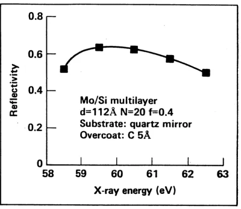
Similarly, in Figure 1.4, the reflectivity drops from 60% to 50% when the wavelength changes by 3.4%. In addition, the focusing optics still in its infancy for multilayer mirrors
0.6
0.4
k-0.2
due to its rigid geometry.
Figure 1.4 Reflectivity vs. X-ray energy plot
The reflectivity of a multilayer soft x-ray mirror is plotted against the incoming light's energy. The peak of the mirror's reflectivity occurs for incoming light with a wavelength of 209 angstroms
(Courtesy of Ceglio N. M.)
Whispering gallery mirrors, on the other hand, are broad band soft x-ray mirrors. Material's Cooper Minima, at which the maximum reflectivity can be achieved, occurs at a wider range of wavelengths compared to the narrow, specific wavelength for absorption edges. This property is what makes whispering gallery mirrors broad band and versatile as compared to multilayer mirrors. As we can see in Vinogradov's data (Figure 1.5): for Rh,
5-
0.8-0.6
0.4
-Mo/Si multilayer
d=112A N=20 f=0.4
0.2
_
Substrate: quartz mirror
Overcoat: C 5A
0
|
1
1
1-58
59
60
61
62
63
the reflectivity only drops from 65% to 55% when the incoming light's wavelength changes by 8.3%.
30
60
90
120
Figure 1.5 Vinogradov's Data
Vinogradov plotted the reflectivity of a whispering gallery mirror with 180 degree or 90 degree turn. The reflectivity of mirrors with 180 degree turn is approximately the square of the reflectivity of mirrors with 90 degree turn
The reflectivity decreases gently to 20% only when the incoming light's wavelength changes by as much as 25%.
We will first examine, in Chapter 2, what has been done in the design of the whispering gallery mirrors. Theoretically, the idea has been studied widely for acoustic waves. Lord Rayleigh pioneered the study of whispering gallery modes. Experimentally, on the other hand, it has only been carried out recently for soft x-rays by Vinogradov of P. N. Lebedev of Physics Institute.
The major literature review of the study of whispering gallery modes is extremely mathematical. It can be found in the appendices. Readers who are only interested in getting a flavor of what the "whispering gallery" mirrors are need not skim through this section.
In Chapter 3, both practical and theoretical design issues are discussed. A design on size and the shape of the mirror is discussed in the first section. The size of the glancing angle is determined by the optical constant of the material at their particular Cooper minimum wavelengths. In the third section, we study, from two approaches the effect of perturbations from a perfectly smooth surface on the mirror's reflectivity. The requirement for our implementation is also described. In the last section, the Kramers-Kronig analysis, which will be used to calculate the optical constants of the materials, is described. This section also has a table of all elements that displays Cooper minimum in the wavelength range that we are interested in. Their properties are listed so that we can examine which element should be used over the others.
We would like to write a program to analyze the 2D Helmholtz equation. A progress report is included in here as to how have we been manipulating the Helmholtz equation. The first section examines the high frequency approximation, which, physically correspond to the x-ray mirror design. The second section examine the low frequency approximation, which, physically correspond to the infrared waves. We also present another approach to solve the problem, the gradient method, which is useful for solving heterogeneous boundary conditions.
In Chapter 4, we examine the issues involved in implementing the mirrors. We examined what Perkin-Elmers has done in building the Space X-Ray Telescope. They have achieved a surface smoothness of 15 angstroms on the average. We will discuss what it would take to
build the whispering gallery mirrors locally. The measuring techniques are also discussed for both approaches.
Issues that are yet to be investigated are discussed in Chapter 5. Whispering gallery mirrors places stringent requirements on the quality of the surface. Large companies, such as Perkin-Elmers, have successfuly built the x-ray telescope. However, such procedure has not been commercialized. We have only been able to find one local industry to undertake such a construction.
II. Present Status of the Whispering Gallery Mirrors
Presently, x-ray optics utilizing the whispering gallery sliding modes have only been built and tested by A. V. Vinogradov at the P. N. Lebedev Physics Institute. Vinogradov have tested whispering gallery mirrors for wavelengths range from 10 to 120 angstroms. For mirror of rotation angle of 180 degrees, he has achieved close to 70% reflectivity (or close to 50% for 360 degrees) for wavelength of 120 angstroms using a Rh coating. The material that coats the mirror is rhodium, Rh. He has also tested other material coatings such as Ag, B, In, La, Ba, LiF, and Be for different wavelengths.
Lord Rayleigh' was the first one to study whispering gallery modes in wave propaga-tion. He pioneered the mathematical analysis, such as the high frequency expansion of the Bessel functions, needed to analyze such problems. He solved the problem for both per-fectly conducting and lossy boundary. Recent important work includes ones accomplished by: Wasylkiwskyj3, Ishida & Felsen4, and others explore further into the problems. The
boundary geometry so far treated are all cylindrical. Bahar5, in solving wave propaga-tion problems along irregular soil surfaces, formulated mathematical expression studying boundary that is consisted of different radii of curvature. Even though Bahar treated a more general problem, his mathematical expressions are hard to manipulate.
In this section, we will examine briefly what each of them have accomplished in the analysis of whispering gallery modes. Detailed derivations, done by Lord Rayleigh, Wa-sylkiwskyj, and Bahar, can be found in Appendix A, B, and C, respectively, for interested reader.
After this literature review, we will outline the problem that we are interested in solving: electromagnetic (EM) field on an arbitrarily shaped surface. We will outline the problem at the end of this section. What we have accomplished so far in solving the problem will be found in Chapter 3, Section B.
II.1 LORD RAYLEIGH'S FORMULATION
A whispering gallery mode, a hump of energy as shown in Figure II.1.1,
Sur face of the mirror
Intensity of the
lin(z)
Whisper Gallery Mode
Figure 1I.1.1
The intensity of a whispering gallery mode is described by the square of a Bessel's function. The closeness of the hump of energy to the surface of the mirror is what made Lord Rayleigh call it a "clinging" wave. is described by Lord Rayleigh as a field that "clings" around a concave
surface. Lord Rayleigh pioneered the mathematical description of the trapping of the high frequency fields inside cylindrical surfaces. He first described how high frequency
waves (in his experiment, a bird call) propagate around the dome of St. Paul's cathedral with exceptionally low loss. However, he did not analyze mathematically the phenomenon until 30 years later(in 1910). He first analyzed a perfectly conducting surface.' He later treated the problem for a lossy medium.2 His analysis of high frequency fields paralleled
his analysis of the waves traveling on a membrane, a problem that he had already analyzed mathematically in his Theory of Sound.' Nevertheless, he needed to take the higher order expansion of the Bessel functions, a technique which was only just developing at the time when he published his mathematical analysis. In our application, we use smaller structures to achieve the similiar effect for the much higher frequency x-rays.
A wave which travels around a cylindrical surface can be described in terms of a Bessel function
w(r, 0, t) = AJ (kr) cos(kct - nO) (II.1.1)
where w is the displacement of the membrane, which parallels the E field in our analysis and Jn(kr) is the Bessel function. The acoustic wave travels with the velocity c, and
k = 27r/A. The waves oscillate around the cylinder with a discrete number of wavelength. We will explain why the waves have such dependence. w satisfies the wave equation,
d2w 1dw 1 d2W
d2+ + + k2w2 = 0
(II.1.2) dr2 +r dr r2 d02 kW=0
w is harmonic in time and can be expanded into a Fourier series:
w(r,6,t) = wm(r)cos[m(O +
am)]ek**
(II.1.3a)dr2 r dr ( cosm(O+ C)w am)=0 (II.1.3b)
If we multiply this sum by cos[n(O + a,)] and integrate it with respect to 0 from 0 to 27r, we obtain,
d2w. 1 dw 2 2
dr r r dr r dr22 (k r2 )Wn = 0 (1I.1.4) which is Bessel's equation. There exist two distinct solutions to Bessel's equation (a regular and an irregular solution). We will use the regular solution (J,(kr)) because the other solution becomes singular at the origin. The index of this Bessel function n takes on integer values because the waves have to retrace themselves around the cylindrical surface. Therefore, we can express Jn(kr) in the following form:
J,(kr) = - cos(n sin 0 - kr)di (II.1.5)
7r 0
The boundary condition for a perfectly conducting surface is
Jn(kR) = 0 (II.1.6)
The "whispering gallery" modes correspond to the first zero that occurs away from the surface.
For a lossy medium, the approach for solving for the transmission of the displacement on the membrane w, which parallels the E field in our analysis can be shown to be (Appendix A)
27rpa -2,.(P-hsp)
Transmission = 1 - re - (1.1.7)
np
where t is the ratio of the refractive index of inside with respect to the refractive index of the boundary (outside); a and p are the densities inside and outside the surface respectively; and
#
obeys the relation: z = n cosh/3. If n is big, i.e., the frequency is high the damping is not significant. Moreover, the less curved the surface is, the smaller y needs to be.Therefore, for a lossy medium, the whispering gallery effect may still persist given that the frequency of the waves is high enough.
11.2 WASYLKIWSKYJ'S FORMULATION
Green's functions are kernel functions used to describe electromagnetic radiations. Its mathematical representation provides a pleasing and accesible way to describe the EM fields. Wasylkiwskyj analyzed the high frequency fields on a perfectly conducting surface excited by a line source using Green's functions.' He pointed out that to analyze the fields that are excited by a line source we can, as a first approach, use ray optics. We shall collect the field solutions for rays that have been reflected one time, two times, - -. It is unlikely, however, that this infinite series will provide any numerical insights.
Another way to sum over all the contributions is to use the whispering gallery modes to collect rays that have the same angle of incidence. However, there is only a finite number of such whispering gallery modes, and they are not sufficient enough to describe all the rays emitted from a singular source. The remaining rays constitute a spectral integral which we shall derive shortly.
Wasylkiwkyj used a perfect absorber to enclose the cylindrical surface to absorb any rays that might have been reflected from the plane. The absorber generates some spurious waves. This spurious contribution is small and can be identified.
Through mathematical manipulations, Wasylkiwkyj transformed the Green's function into a ray optics and/or whispering gallery mode representation of the fields. He identified the accuracy for each representation. Therefore, as developed in a later work by Ishihara
and Felsen, it might be necessary to use a combination of such representations to describe the fields.
1. The Whispering Gallery Modes and the Continuous Spectrum Integral Representa-tion
The Green's function's angular dependence assumes the form:
exp(iv0
4
- 01)g0(0 1o; V) = -
)(I.2.1)
-2wv
where 0 denotes the angle at which the source point is located and V is the propagation constant of the waves.
The Green's function can be expanded into a set of eigenfunctions:
G(f
fo)
=Ego
(0
1o;
v) 0,(r) bL,(ro) (11.2.2) (11.2.2) satisfies the wave equation for a cylindrical surface:(1
a
182 2 = 6(r - ro)6(4 - Oo)r- + + k) G(f Io) - (II.2.3)
rr
o
r r2ag02rThe perfectly reflecting surface has the boundary condition,
=G(f
0) = 0 (11.2.4)
49r r=a
with a as the radius of the cylinder. We obtain, for the Green's function:
. N ika -00
G ( a ,
4
, o ) =-kan (7r/2 - wn) cos w,
00
dye-
c 0--oIsnh
(11.2.5)
oe -* + 0 (II.2.5
where the first term is the whispering gallery modes and the second term the continuous spectrum integral. The last term is the spurious effect generated by the absorbing boundary condition. Detailed derivation can be found in Appendix B for interested readers.
2. Geometrical Ray Representation
In the geometrical ray representation, we try to represent the Green's function as consisted of rays that bounces off the cylindrical surface 1, 2, - - - , I times. To establish a
geometrical ray representation of the fields, we use a Fourier transform representation of the Green's function:
G(f fo)=
-
e"'1O#O*gr(r ro; v)dv (11.2.6)27r -oo
which we take the high frequency expansion and is shown in Appendix B to be:
G(a,
4,1 40)
~E:(-1)'eiqw/2
-(+1)1 (11.2.7)L-1
3. Geometric Optics and the Whispering Gallery Modes Representation
Wasylkiwskyj tries to compensate the imperfection in each formulation by using a combination of the the geometric optics and the whispering gallery modes representation, he arrives at the result:
L
G(a,
4, 40)
~E(-1)'e ~/x+)I (a,4, 40)
L=1+ (-)L+1 ei(/2)L+2)FL+1 (a,
4,
0o) (11.2.8)2
M ika -40 sinWn
+ EZ/2 )
ka n_1 (7r/2 - Wn) cos Wn
where the first term is the geometric rays and the last term the whispering gallery modes. The second corrects for the field that is not represented by either of the two representation.
11.3 ISHIHARA and. FELSEN'S FORMULATION
Ishihara and Felsen reconstructed each of Wasylkiwskyj's formulation of the high fre-quency fields on a perfectly conducting cylindrical surface that is excited by a line source. They verified the accuracy of each formulation numerically and developed a representation to explain the fields that are close to the source point."
All formulations except for the whispering gallery modes plus the canonical integral representation fail to explain what happens to the field when the observation point is close to the source point. The ray optics representation fails miserably when the observation point gets close to the source point. This is so because when we try to get close to the source point, numerous caustics are formed. Even if we try to scrape up the contributions from those caustics by collecting them in an integral expression, the integrand is shown to diverge. The whispering gallery modes and the ray optics representation, on the other hand, do not explain what is on the surface field either. The ray optics terms in this representation, again, diverge when the observation point gets close to the source point. We shall resort to the integral expression of the field,
_1e~
G(If fo)=d
(I.3.1)
i(rka)2 IeH (ka) J,(ka)
After we take the respective contour integral and plug in the appropriate Wronskian
relation, (11.3.1) is shown by Ishihara and Felsen to reduce down to
eik* ka 2/3
G~ -
-2irka 2
I
-o-iS +oo-is e Ai(t)dtAi(t)ka
( / S2 a (II.3.2a)
and
(II.3.2b)
Part of the integrand in (11.3.2) can be shown to be expanded into
Ai(t) Ai(t) 10 )/ + 0(t-34/2) j=0 I -7r < argt < 0
By Laplace's inversion, (11.3.3) can be expanded into the terms
G~H 1)(ks) { bjT(3/2)j + 0( 3 3/2)
2 Ij=0
The coefficients in the series are given: b0 = 1 bi = iei/4/4 b2= -7i/60 b3 = -7-resr/4/512 b4 = -. 4398134 x 10-2 b5 = -. 4109687 x 10~3geir/4 b= .1122861 x 10-3i b= .9182121 x 10-5 Fe "/4 b= .2093046 x 10-' b9 = .1637812 x 10-6/7e i/4
[ 1
where (11.3.2) (11.3.3) (11.3.4)bio = -. 3633427 x 10-7i
iH(1)(ka)/2 is the Green's function for a perfectly conducting plane.
To analyze the case in which the surface changes from concave to convex while the distance of the convex surface remains the same, we let a change continuously from 0 to 2ir.
The whispering gallery mode and continuous spectrum representation gives accurate results except for low ka values, where the whispering gallery eigenfunctions are difficult to be evaluated. In the near field, values are (as previously pointed out by Wasylkiwskyj) dominated by the Neumann's function and the whispering gallery modes.
The whispering gallery mode and canonical integral representation, on the other hand, serves as a good reference for low ka values for the near field calculation. It does not exhibit the whispering gallery mode calculation problem as in the previous representation. The combination of rays and whispering gallery modes, as calculated by Ishihara, provides a good approximation for length within the inequality. For observation points very far away, we have to include a large number of whispering gallery modes. Therefore, the representation becomes hard to calculate.
II.4 BAHAR'S FORMULATION
E. Bahar analyzed the high frequency field on a surface that is of both varying impedance and curvature.' This is a more general approach than the one undertaken by Ishihara, Felsen, and Wasylkiwskyj. However, Bahar did not generate numerical results.
Bahar describes a surface of arbitrary curvature and variable impedance by x, y, and
z.
The coordinates are defined in the following way: Surfaces on which z are constant are normal to our surface; surfaces on which y are constant enclose the surface (y > 0, when y is outside our surface); surfaces on which z are constant are normal to the axis of the cylinder.
The x, y, z coordinates are related to the cylindrical coordinates in the following Jaco-bians: ar ar dR J -a y _ z- (II.4.1a) !M 2± 1- O am ay R am 8: 0 R JT= _ r - (II.4.1b) 1y RdR ar a4 dz
The Maxwell's equations in cylindrical coordinates can be made to depend on x and r while eliminating the
4
dependent component of the magnetic field. We obtain:?x W H, (II.4.2a)
5T Rr
8H, . r
1
8
(r
aE,]
r--
ax
= IR E, + k-2 or k25-r
R - + -J, B- (II.4 .2 b)where k = w(pIE)1/2 and J, = rS(r-ro)6(,-Zo)
R
For the cylindrical case, where r = R, E, satisfies the following scalar wave equation:
1ia
8E
1
a2E
V2E, = r-(r
)
+- + k2E, = impJ, (11.4.3)
E, can be expanded into the following eigenfunction expressions for zero impedance.
E,(, 4 = FH2 ( o)Hj () X
H,(,) (e) cos vn (4 - 40 - 7r)(144 8H. (2)(g)) sin y,,
av M.
where H' 2)
(
) are the Hankel functions of the first and second kind and that andCR denote the number of waves in the specified radius.
The electromagnetic fields satifies the impedance boundary condition at r = R,
aE. n Ez(II.4.5)
d(kr) Z.
where r1 is the intrinsic impedance of the medium. Each order vn of the basis functions satisfy the equation
H (t) - !H7 )() = 0(11.4.6)
We can write the azimuthal dependence of (11.4.4) as a superposition of the forward traveling and backward traveling waves:
E(e, x) = [an(x) + b.(x)] (11.4.7)
We can express the magnetic fields in a similar way:
00Y (e)H()
H,(,z) {an(z) - b (11.4.8)
n=1
The forward traveling waves, as noted before by Lord Rayleigh and others, constitutes not only the direct wave propagating in the positive x direction but also the whispering
gallery waves which propagate around the cylinder p times (p is an integer).
After a number of manipulations, we obtain for the amplitudes of the traveling waves:
a.(z)
=f
ao(u) x
exp
(+
()dv] du (11.4.9)= o dTu i d
Rv]
11.5 WHERE DO WE GO FROM HERE
Using mathematical tools, such as the contour integral, WKB method, and asymptotic expansion of the Hankel functions to obtain the Green's function, Lord Rayleigh, Wasylki-wskyj, Ishihara and Felsen, and Bahar have exhausted the development of the Green's function for a cylindrical surface in the high frequency limit. We now outline the approach that we propose to take in solving this problem.
To determine the electromagnetic field in the region of an arbitrary shaped surface containing a high frequency source, we need to use the Huygen's principle. Given that we know the field or its normal derivative everywhere on a closed surface, the Huygen's principle tells us what the field is everywhere inside the surface. We shall rederive it in Appendix A.
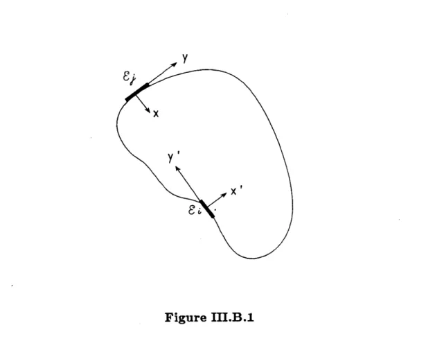
The following technique will be used to apply Huygen's principle: we divide the surface into small finite elements (Fig. 1). The field on one finite surface element can be found by summing over the contributions from all other finite element surface fields weighted by a Green's function. The source surface element has an additional source term. If we let E denote either the field itself or its normal derivative, then
E; =
EG;;Eg
i = 2, 3, 4, -.--. n1j
j 19213,..,n (II.5.la)
Ei =
EG
1 E, + Sj
= 2,3,. -, n (II.5.1b)i jo1
where Gij is a Green's function that associates surface i to surface
j
and S is the source term.If we know what the Green's functions are, we can solve for the E fields on the surface by solving (11.5.1) self-consistently. However, each finite surface element is large compared to the wavelength of the field.
Recently, we have found literature from Check Lee of Prof. J. A. Kong's group that analyzes the problem of the arbitrarily shaped surface. Check Lee is also working on this problem. The approaches taken by Check Lee and authors of the literature are slightly different than the one we have just described.
The Huygen's principle is derived in Appendix A to establish the theoretical basis of our analysis. We also derive the eigenfunction expansion of the Green's function (Appendix B) because we need this tool to study a light source composed of more than one mode. We shall explore the solution for the Green's function for an arbitrarily shaped surface further in Chapter 3.
III.A.1 The Size and the Shape of the Whispering
Gallery Mirrors
It can be shown that the whispering gallery modes are insensitive to the size of the mirrors to the first order. In other words, the reflectance of the whispering gallery mirrors does not depend on the size of the mirror. The geometry of the inner surface, (See photograph of the mirror) determines the number of focal points (See Figure III.A.1) If we wish the
t- .- v=sa ,Vy.y 1- 10 .
wqw ~ aadsenraae wm p = M s .- -aeat
SLrar t e V.asha #c. Bh"ap ass P.ee ma ,"r . 12As Playt o -"d Lh. 11 an 13 p 1047.re h
light beam to focus only at the endpoints of a 360 degree turn mirror, we use elliptical
8B.
Figure III.A.1 Whispering Gallery Mirror's Focusing Optics
Focusing optics of the whispering gallery mirrors is determined by the geometry of the inside surface. The inside surface of a 360 degree mirror is shown in the figure. A. Elliptic : the focus occurs at the two endpoints; B. Spherical : the focii occur in the center and the the endpoints; C.
Toroidal : the number of focii is determined by the toroid's radius of curvature.
F7m
surface (A in Figure III.A.1). Spherical surfaces can focus at two points (B in Figure III.A.1). Three or more focal points will require the inner surface geometry be toroidal, with different curvature of radii.
Since the reflectivity of the whispering gallery mirror is independent of the size of the mirror, we can vary the size of the mirror to accomodate the light pulsed that comes in. The size is designed to be at 10 cm diameter to fit the envelope of 15 pulses that comes in. The pulse is 30 nanosecond in duration.
III.A.2 Glancing Angles
In the x-ray regime, all materials' indices of refraction differ little from unity, that is,
n = 1 - 6, where 6 is a small number1. In other words, for a beam of x-ray, the vacuum, whose index of refraction is unity, is optically denser than any material
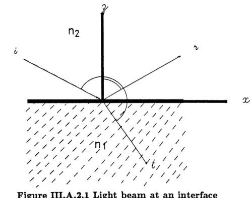
Figure II.A.2.1 Light beam at an interface
Incoming beam, i, coming at an angle Oi from material with index of refraction n2, hits a ma-terial with index of refraction ni. Part of the beam is reflected and the other part transmitted.
considerable amount of reflection of x-ray will occur. Because n differs little from unity, this critical angle is extremely small. Those small angles have been referred as grazing incidence angles or glancing angles2 9.
The light rays in Figure III.A.2.1 obeys the Snell's law which states that the sine of the transmitted angle of the light ray isio proportional to the sine of the incident angle of the light ray by a proportion of the refractive indices of the two materials:
sind, = -sinO; (III.A.1)
nl2
As stated above, all materials indices of refraction becomes less than unity in the x-ray regime. Therefore, there exist a critical angle 6, at which the transmitted angle Ot becomes parallel to the interface and the power of the light ray transmitted become an exponential
decay,
0C = sin-n2 (III.A.2)
In the x-ray regime, the ratio n is very close to 1. The critical angle, 0,, becomes closer and closer to 90 degrees. The incident ray is grazing the surface of the mirror.
If the index of refraction is complex, so that
k = k, - ki (III.A.3)
the field attenuate exponentially into the material.
E = Eoe~kiz (III.A.4)
where z is the depth of the material. Penetration depth of the material is defined to be
d, = (III.A.5)
where the field has become of its original values. If the incoming light beam is 200 angstroms, copper's index of refraction is .96 + i.10. Its skin depth would be 10 angstroms. For nickel, the index of refraction for the same wavelength is .98 + i.09. Its skin depth would be 11.1 angstroms. For silver, its index of refraction is .88 + i.21 which leads to a skin depth of 4.76 angstroms.
III.A.1 The size of the glancing angles and beam height
Let us assume that the material has its real part of the refractive index .999, its critical angle is 2.6 degrees, the height of the beam for a mirror with the radius R, is equal to, (by simple geometry) R[1 - sin,]. If the radius is 5 cm, the beam height would be - 51p.
III.A.2 Absorption of soft x-ray in air and one-bounce experiments
It is necessary to work in a vacuum chamber for soft x-ray experiments, because x-rays' penetration depth of an impure environment is very shallow.
In experiments, physicists have dealt extensively with one-bounce experiments to obtain the optical property of the materials"-". Multiple-bounces, as required by the whispering gallery mirrors, have only been carried out extensively by Vinogradov.
III.A.3 Theoretical problems associated with glancing angles
Glancing angles treat the "particle-like" picture of the x-rays. If we work with the particle model, the picture is follows: on each bounce, there is some loss associated with
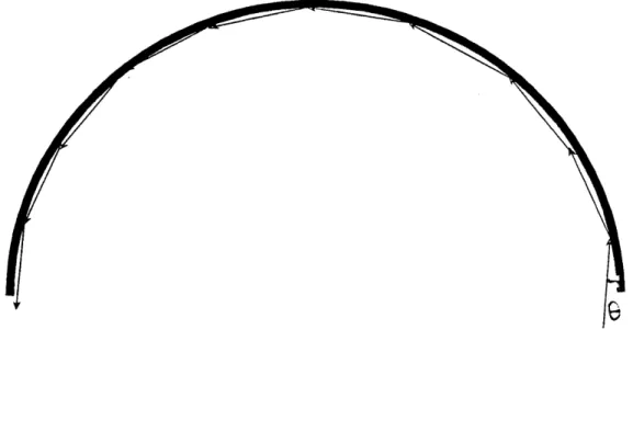
it, the total reflectance of the mirror is consequently dependent on how many bounces there is, and thus dependent on the mirror's size. We can calculate how many bounces that the light particle coming in at an angle 0 and turned by a mirror of angle (. Each bounce of the particle encompass twice the incidence angle. Therefore, by simple geometry, we can see that the light beam make approximately j bounces. If the incoming beam is .54 degree
Figure III.A.2.2 Sliding Angle Graph
The incoming light beam, denoted by the arrows in the figure, comes in at a shallow angle 6.
and that the light beam is turned by 180 degrees. The beam would have bounced off the mirror approximately 100 times. Suppose the reflectance of each bounce is 99.7%. The intensity of the beam turned by this 180 deg mirror is approximately 74% of the incoming beam.
III.A.3 Perturbation Analysis of Surface Roughness
of the Whispering Gallery Mirrors
It is imperative to consider the effect of the irregularities that are left on the surface have on the reflectivity of the whispering gallery mirrors because they exist inherently in any polished (or superpolished, for that matter) surface.
We can model the imperfect surface as a perfectly smooth surface that has a Gaussian distribution of irregularities with a correlation radius, a and a height, g.
It is shown by Vinogradov by solving the solving a two dimensional Helmholtz equation adding the surface irregularities as perturbation terms, that the reflectivity of a bent surface mirror is 1
R2 = R|2 - b1R|2 = |R 2 1 - 4k2 2 2 (12 ) (III.A.3.1)
where R is the reflectivity of the bent surface mirror, el is the permittivity of the mirror,
0 is the angle of incidence, and k is the wavenumber. p. is a measure of the size of the
incidence angle. a is incorporated in the expression p. It is equal to:
1 ajkE 2
p= ak?6
4
The expression 4 (p) can be evaluated for two limits: either L >> 1 or y < 1 1
( = t
1
= 1 - +
-16p2
2 i
[r
( )
+
2 \)
(III.A.3.2)
If the incidence angle is extremely small, as in the case of x rays, Eq. (III.A.3.1) reduces
R'=
|R1
2 1-E(4
(III.A.3.3)
7r 2 (ka)2
For whispering gallery mirrors, we can represent the propagation of the x ray beam as a series of reflections off the mirrors. Consequently,
IR(6,
4)|
2=
|R(O)I
(III.A.3.4)There are a large number of reflections. In such limit, Eq. (III.A.3.3) can be shown to transformed to the following expression,
R(, = exp
[-
(1 - IRI2 exp -44 p(/I> (p) (III.A.3.5)For grazing incidence angle, where a - 0, the surface is considered smooth if the following condition is satisfied:
(III.A.3.6)
Since our wavelength is larger compared to correlation radius, we can choose smaller correlation radius, say greater or equal to 1 p. For incoming light with a wavelength of
D
k 3 ' < a - 44
J
200 angstroms hitting a surface with correlation radius of 2 y, the irregularities' height should be less than 100 angstroms.
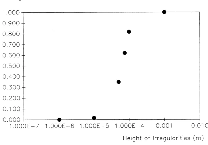
Let us calculate the loss of reflectivity due to scattering, which is described by the second exponential term in Eq. (III.A.3.4), for the example just mentioned. There is also losses due to photoabsorption. Let us consider for a mirror that rotate the incoming light beam 180 degrees. If the height of the irregularities is 100 angstroms, as we can see in FigureIII.A.3.1, the loss due to scattering is 82%. Let us assume that loss due to absorption is 30%. The mirror's reflectivity would be 5.4%. If the height reduces by a half to 50 angstroms, the loss due to scattering will have decreased appreciably to 34.8%; the mirror's reflectivity would be 65.2% x 30.0% = 19.5%. The scattering becomes closer negligible, when the height reduces to 10 angstroms. The surface's scattering losses are
sensitive to microirregularities with the height between 10 and 100 angstroms.
Scattering Loss
1.000-
0.900--0.800
--
0.700-0.600
-
0.500--
0.400--
0.300--
0.200--
0.100--0.000-
|1.OOOE-7
1.OOOE-6
1.OOOE-5 1.OOOE-4
0.001
0.010
Height of Irregularities (m)
Figure III.A.3.1 Scattering loss vs. Height of surface irregularities
Assuming the correlation radius is 2 y, the height of the surface irregularities is plotted against scattering loss. For a surface with irregularities of height less than 10 angstroms, it can be considered scattering loss free.
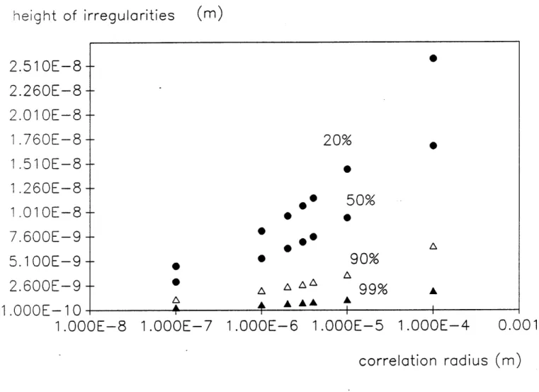
In Vinogradov's example, the incoming light beam is also 200 angstroms in wavelength. He rotated the light beam 90 degrees. His surface's microirregularities were 60 angstroms in height rms. He considered the surface to be smooth if the correlation radius g is >
irregularities' height and correlation radius.
height of irregularities
(M)2.51 OE-8
2.260E-8
2.01 OE-8
1.760E-8
1.51 OE-8
1.260E-8
1.01 OE-8
7.600E-9
5.100E-9
2.600E-9
.000E-10
1.000
E-8 1.OOOE-7 1.OOOE-6 1.000 E-5 1.OOOE-4
0.001
correlation radius (m)
Figure III.A.3.2 Height vs. Correlation radius
The values of surface irregularities' height are plotted against their correlation radius for different (1 -scattering loss).
Practical issues that are involved in reducing microirregularities can discussed in Chap-ter 4. Obtaining smoothness on the order of hundreds of angstroms is easy. Obtaining smoothness of 10 angstroms require much more work and have only been carried out by very few industries.
20%
0 ,* 50% * , 0 0 0 90% A99%
AIII.A.4 Kramers-Kronig Analysis
The real part of the optical constant is related to the imaginary part of the optical constant by the Kramers-Kronig relation1(50).
n,.(w) - f iW d (III.A.4.1)
Therefore, if we know the real part of the optical constant, we also know the imaginary part and vice-versa. Kramers-Kronig have been used extensively to calculate the optical constants theoretically. It provides a good estimation for the energy range that we are interested in.
For energy above 100eV, the relationship for finding the optical constants become much simpler. The relationship is linear2. If we write the dielectric constant as a complex constant e:
b and # are related to the atomic scattering factor
f,,
b
=()
A X20EXPfip (III.A.4.2)3 = ( A2
4
zxpf2p (III.A.4.3)
where
fi,
and f2p designate the real part and imaginary part of the scattering factor, respectively and4
is the number of molecular groups per unit volume each with x, atoms.The experimental data for photoabsorption cross section for 100eV and above have been compiled by Henke, B.L. for all elements2. Therefore, the optical constants can be much more easily obtained for energy of that range.
III.A.4.1 Kramers-Kronig's relation
We have been setting up the program to use Kramers-Kronig to calculate the optical constants of all material at energy range below 100eV. We describe the Kramers-Kronig briefly below.
The analyticity of the optical constant, ic, in the upper half plane of w allows the use of the Cauchy's theorem to relate the imaginary and real parts of ic as shown in Eq. (III.A.4.1). The real part of the optical constant is related to the total cross section at
1c,(2) -1=02--PW 2dw (III.A.4.1.1)
where the total cross section is composed of both the absorption cross section, o, and the scattering cross section, a, 3
at = Ga + a, (III.A.4.1.2)
The scattering cross section can be shown to be negligible compared to the absorption cross section. Consequently, we shall worry only about contribution due to only the the absorption cross section. We can rewrite Eq.(III.A.4.1.1)
IC,(W) - 1 s 2 -- P ,2 2 dw(III.A.4.1.3)
?A 0o 12- W
The equation becomes singular at w. We can resolve this singularity by subtracting the singular value from the integrand,
(W) - W) * + W d &0'(III.A.4.1.4)
The first term can be calculated by numerical integration, and the second term can be evaluated analytically. In addition, we will truncate the integration interval for the first integrand at which the absorption cross section starts to decrease.
Most photoabsorption cross section may have steep slope. To approximate such high rate of change, the quadrature that we use will follows Simpson's i rule.
III.A.4.2 Utilization of the Cooper Minimum
For a specific wavelength that we wish to design the mirror for, we want to use elements that has their Cooper Minimum at that or close to that specific wavelength. Basically, Cooper Minimum is the point at which the photoabsorption cross section of the element is at its Minimum. If the element absorbs less, it reflects more.
J. W. Cooper used a nonhydrogenic model with central field to describe the absorption-edge-like phenomenon in lower energy (between threshold and a few hundreds of eV)4-7. Cooper Minima is due to the zero of the photoionization matrix element. It is an interfer-ence effect.
For 200 angstroms, which correspond approximately to 64eV, both thorium and barium
displays a Cooper Minimum at that energy level. (See Figure III.A.4.1) -
1
________ ~ F=El! 200.. 10 100 E (eV) 1000 0,000 10 100 E (eV) Figure III.A.4.1The Cooper Minima, which occur at less than 100eV for both Ba, plot on the left, and Th, plot on the right has a much gentler slope than the absorption edges, which appear as sharp peaks at the higher energy levels.
III.A.4.3 Selection of material for our WGM mirror design
The wavelength for which we want to build a whispering gallery mirror for is approxi-mately 195 angstroms.
The following criteria are used in narrowing down the elements. 1. It should not be radioactive
2. It should not oxidize easily (especially on the outer few angstroms, because the skin depth is on the order of angstroms)
3. It should serve as a good thin film coating (malleable; not brittle)
Besides the criteria cited above, the element should be within budgetary constraints. Of all the elements listed, none of them is beyond reach. Some elements are toxic. However,
f2t
80
since highly toxic elements, such as Ga and As, have been successfully handled in labs, toxicity does not serve as a major criteria.
The following survey shows the properties of the elements that has their Cooper Min-imum in the soft x-rays.
The final three elements that we are considering are molybdenum, strontium, and zirconium.
Element toxic oxidizes in air radioactive brittle 36 37 38 39 40 41 42 43 44 45 46 47 Kr Rb Sr Y Zr Nb Mo Tc Ru Rh Pd Ag Cd In Sn Sb Te Xe Cs Ba La Ce gas liquid ductile ductile no 178A 155A 153A 104A 113A 113A 116A 146A 116A 116A 88.8A 96A no no no no no no no no no no no no yes low no yes yes no no no yes low-med no \relax
Z
physical forms krel N/A no yes yes yes no yes no no no yes no high temp no no yes high temp no no no no noair with ozone and sulfur no no yes no low temp no high temp no yes yes no no N/A no yes no yes no yes no yes no N/A no no no no no no N/A no no no no no no no no no no N/A N/A yes no no 83A wets glass 73A
78A
62A 62A volatile 62A gas 249A liquid 244A 191A 173A 155A 48 49 50 51 52 53 54 55 56 57 58---59 60 61 62 63 64 65 66 67 68 69 70 71 72 73 74 75 76 77 78 79 80 81 82 83 84 85 86 87 Pr Nd Pm Sm Eu Gd Tb Dy Ho Er Tm Yb Lu Hf Ta
W
Re Os Ir Pt Au Hg TI Pb Bi Po At Rn Fr no low-med no unknown no no unknown no low-med no no low-med low yes no no unknown no no no no yes no yes no no no no no yes yes no high temp yes moist no no moist no moist yes no high temp high temp yes no no no no no no yes no no no no N/A no no no yes no no no no no no no no no yes no yes no no no no no no no no no no yes yes yes yes no no N/A no no no no no no no no no no no no no no yes yes no no N/A no no yes no no N/A N/A liquid costly costly ductile liquid volatile gas liquid 124A 105A 138A 153A 178A 88.8A 85.7A 88.8A 82.9A 113A70.6A
248A 137A 178A 155A 155A 124A 138A 143A 105A 95.6A 77.7A 77.7A 76.3A 67.2A 62.2A 59.8A 296A303A
Ra Ac Th Pa U Np Pu no no no yes no no no yes yes yes yes yes yes yes synth. synth. 31
oA
248A 204A 141 A 132A 143A 138AIII.B Theoretical Design of the Whispering Gallery
Mirrors
III.B.1 Finite Element Analysis of 2D Helmholtz Equation for An Arbitrarily Shaped Surface
In our design, we want to solve the Green's function for an arbitrarily shaped surface. We will do so through a finite-element approach. We cut a surface into small pieces. On each piece, there is a field Ej associated with it. To visualize the E field more easily, we can define a new set of coordinate for each piece. (1 is parallel to the piece; 2 is normal
to the piece1-3
Figure III.B.1
An arbitrarily shaped surface can be described by finite elements. A new set of coordinates, one is normal to the finite element, and the other parallel, can be defined to describe each element
where they are transformed from the x and y axis in the following way:
el= zcosi + ysin/
2= -Xsin) + ycosk
According to the Helmholtz's equation, the contribution of E to Ej is
Sa eik-[(C1-$1) 2+ (2-4 2j) 2
+Z2
e ik[((e1-i,) 2+(2-2) +,21 2 dE (, () (III.B.1.1)
[(e1 - 1s)2 + ( 2 - 2i)2 + Z2]
dC
where we have assumed that the field does not vary along the z-axis. As stated by the Huygen's principle (as mentioned in Appendix D), if we know how each piece is related to one another, we can solve for the E field on the boundary and within the surface by solving each of the piece self-consistently. At this point, we will concentrate on simplifying (III.B.1.1) rather than solving the matrix itself.
We can rearrange the terms in (III.B.1.1),
69 f oo eik[((1- _ig)2 +(62-62j)2+Z2]2 E;(j)( (2) = d(2Ej((1, W2 dz -(6
01
-, ( _ 2 + (e2 -0)
2 + Z212 - dE(
) 0iL +(62-62)ei(e]-ktI12 2 +,2)+ - de2 f dz()
(III.B.1.2)We
di
-o*[(1
valu)2t+ (t2 - 2e)2+
2r2We can evaluate the expression along the z-axis. We are evaluating the expression,
Since variables (1 and C2 substitution,
00 ik{(f]1-(1g)2+( C2-C2j )2+X21 j
[(ej . dz (III.B.1.3)
1 ~~,) 2 +
(6
-C2)
2 + Z212
act as constants in this expression, we can make the folowing
a2 =(e 1 )2 + (e2 - 2) 2 Equation (11.3) becomes,
00
_eia 2+Z2] I -co(a
2+
z2)
We can expand the exponential into cos's and sin's,
f
dzeskt 2+z211~ -00 i~foo z cosk(as2 + Z2)1/2
=
f
W
+
J-oo (a
2+
z2)
1/2 dz cosk(a2 + 22+
2i(a
2 + Z2)1/2 +f
dzsink(a+
z)1/2 - (a2 + z2)1/2 00 dz sink (a2 + Z2)1/2 o (a2 + z2)1/2due to the integrands' evenness.
We can make another substitution to simplify the integral. Let
U 2 2 2 (11.5) becomes, 2 d u cosk u 2]
(u
2 -2 (U a2)2+
2if du sinku a (U2 - a2)2 Equation (11.6) is evaluated to beNo(ka)
+iV/r
Jo(ka)
an expression that can be simplified to the Hankel's function expression. (11.3) is equivalent to
inrHo(ka)
We can substitute
(II.7)
back into our original equation, we arrive at- i7rHo(k[(
1
-el1 e15)2 + (62 - e2;)2])
- dE ( ( 2) -iHo'(k[(e1 - (1;)2 + (2 - )
-6d del irH16 ~
Most of the time we are interested in how many wavelengths do each piece contain, that is, we are interested in ka and not a itself. We can substitute the following expressions,
2 = k2 2 Ol7 k( 1 -= 2f 0o E!) (1, 2) = ( III.B.1.5) (III.B.1.6) (III.B.1.7) -f
6de2E (el1, e2)
(III.B.1.8)
(III.B.1.9.1)
Cr = k - 2 )2 + 1j = + 2i 20rida = 2((1 - e15)d(1 2a2da2= 2(e2 - e25)de2 so that, d(1 = , da0 (0) dw2 = a2d2
we can rewrite (II.8) in the following manner:
6J~'
kda
2E,
(ai,Or
2)k
f -k(6-i) kd dE(ai,o2) Jk(-6-CIj) dor1 i rcH
(aa1
[a + ) ,., 2 Hi)({cTi + uj]i)au
1Lf I
(III.B.1.9.2) j = k2( (III.B.1.9.3) (III.B.1.9.4) (III.B.1.9.5) (III.B.1.9.8) (III.B.1.10)III.B.2 Analysis of 2D Helmholtz for High Frequency
Approximations
Essentially, we wish to solve the result we obtained in Section III.B.1 for all frequencies. We want to simplify Eq. (III.B.10). We can take two different approximations: the high frequency approximation and the low frequency approximation. Physically the high frequency approximation correspond to solution for uv or x-rays. On the other hand, the low frequency approximation correspond to infrared light beams.
In this section, let us examine the integral using asymptotic high frequency approxi-mation, we get
6 Ho (k(x - x')) e'"' dx' = dz 8 d'eiteik(-z)CosZ
=
inf
dzetkc**f d'xeik'cosz+iI7z'7r C J-6 1i(n-kcosz)6 _-i(r-kcoz)6 = - dze'**** 7 c
1
- kcosz I if dz i(kzcosz-k6coz+96) _ -ikxcosz-k6cosx+i6) ux c 7 - kcoszIf we evaluate the first term of the integral in (III.B.2.1), we arrive at
1
ei76
f
ei(kzcos"coa) sdz
ix C 17 - kcosz
z is a complex number, i.e.,
z = U + iv (III.B.2.3)
Moreover, we have satisfy the condition that it is constant phase; consequently,
i (kxcosz - kocosz)
isc
(III.B.2.1)