HAL Id: hal-01814170
https://hal.archives-ouvertes.fr/hal-01814170
Submitted on 21 Oct 2020HAL is a multi-disciplinary open access archive for the deposit and dissemination of sci-entific research documents, whether they are pub-lished or not. The documents may come from teaching and research institutions in France or
L’archive ouverte pluridisciplinaire HAL, est destinée au dépôt et à la diffusion de documents scientifiques de niveau recherche, publiés ou non, émanant des établissements d’enseignement et de recherche français ou étrangers, des laboratoires
Capturing the dual relationship between simulation
models and their context
Mamadou Kaba Traoré, Alexandre Muzy
To cite this version:
Mamadou Kaba Traoré, Alexandre Muzy. Capturing the dual relationship between simulation models and their context. Simulation Modelling Practice and Theory, Elsevier, 2006, 14 (2), pp.126 - 142. �10.1016/j.simpat.2005.03.002�. �hal-01814170�
ABSTRACT
Capturing the relationship between a model and the context that prevailed to its building is a fundamen-tal problem in Modeling and Simulation (M&S). Making explicit the objectives, assumptions and con-straints in disguise behind this relationship can greatly help to drive the M&S life cycle better. A sound systemic-based foundation is provided here to achieve this goal in a clear abstract form. To this end, the concept of experimental frames introduced by the DEVS framework is developed thoroughly, through a specification hierarchy. A fire spreading application, which has been specified using this formal frame-work, is shown to illustrate its operational sight. The following benefits suggest themselves from this work: firstly, it is easier to capture and to manipulate some M&S fundamental and advanced concepts, and then to enhance our understanding about them. Secondly, making context specification inherent to the M&S process as a dual part of real system specification will significantly improve the global knowledge. Lastly, the formal framework, with both system and context specification hierarchies, pro-vides a methodological guide to the modeling process.
1 INTRODUCTION
In the traditional M&S process, model building is done by specifying the abstraction retained to describe the system under study [9, 16], without conducting simultaneously the same process for the context in which the system is studied. Yet, the validity of the model can be measured only in this context. Since a model is meaningless without its context, a sound M&S enterprise must drive the specification of both the model of the source system and a companion model of the context of the study. Creating a model for the context is not a current practice in M&S. Which factors can characterize a context? According to [8], there is no agreed framework for these factors. There are similarities between the acts of specifying a model for a real system and specifying a context: only the most significant factors are retained and de-scribed. However, there is a common agreement to recognize that a model of context must make explicit at least the underlying objectives, assumptions and constraints of the study [8, 17]. Such a specification makes it possible to identify models that can be relevantly (re)used within a given context. Conversely, a given model can be checked for compatibility with various contexts. A formal framework in which con-texts can be specified in their clear abstract forms can provide a powerful means to manipulate this com-patibility concept and others that come under the model-context duality. The benefit of the present work is to provide a sound basis for such a framework.
The separation of concerns between a model and its simulator [25] is known to be a fundamental principle in the M&S process. We have formalized a similar separation between a model and its context, as a systematic part of the M&S process. The approach adopted is rooted in systems theory, the DEVS formalism, and the experimental frame methodology introduced by the multifaceted modeling and
simu-CAPTURING THE DUAL RELATIONSHIP
BETWEEN SIMULATION MODELS AND THEIR CONTEXT
Mamadou K. Traoré LIMOS CNRS UMR 6158
Université Blaise Pascal
Campus des Cézeaux, 63177 Aubière Cedex, France Email : [email protected] (corresponding author)
Alexandre Muzy SPE CNRS UMR 6134
Université de Corse
Campus Grossetti, 20250 Corti, France Email : [email protected]
lation framework [22, 23, 25]. The specification hierarchy introduced to this end provides an operational formulation of objectives, assumptions and constraints that prevail in any simulation modeling effort. As far as we know, few research works have dealt with this concern [7, 12] and none with a general formal-ization as those provided by the work in progress [18-19].
Section 2 presents the modeling and simulation framework and underlines the process of translating the system/context pair into a model/frame pair, and then into a simulator/experimenter pair when neces-sary. The frame specification hierarchy is developed in section 3 through three levels. Its effectiveness is shown in section 4, by an application to a fire spread simulation, whose specification and visual results are presented. A discussion is provided in section 5 and concluding comments are given in section 6.
2 MODELING AND SIMULATION FRAMEWORK
The System-Model-Simulator (SMS) view is a well-accepted framework in the M&S community. The SMS view defines the System, the Model and the Simulator as the entities that are central to the M&S enterprise. The two most fundamental relationships that hold between them are the modeling and the simulation relations [25]. While the modeling relation refers to the degree at which the Model faithfully represents the System, the simulation relation refers to the principle of separation of concerns between design and implementation levels. The Experimental Frame (EF) concept has been introduced to catch the set of circumstances under which a system is to be observed or a model is to be subjected to experi-mentation [22, 23, 25].Since modeling is recognized to be context-driven, how can one understand the models’ contextual dependencies accurately and unambiguously? Moreover, how can one reason sym-bolically about model and context matching? Our answer is that both models and contexts must be de-scribed formally, and we suggest context be entirely modeled by EF.
2.1 Frame concept
Experimental Frames have been defined according to the following principle: “Any data gather-ing/reduction (statistics, performance measurements, etc.) or behavioral control (initialization, termina-tion, etc.) that is conceptually not carried out in the real system should not be placed within its model but rather formulated as part of the experimental frame. Conversely, any dynamic structure that is supposed to correspond to mechanisms existing in the real system should be placed within the model” [23]. Hence, an EF is a system that should interact with a model (or a source system), to produce the data of interest under specified conditions. It should be remembered that the EF only specifies a family of ex-perimentations to be done, not any particular one.
An EF is given in [23, pp. 210-211] as a structure <T, I, C, O, ΩI, ΩC, SU>, where T is a time base, I
is the set of input variables, C is the set of run control variables, O is the set of output variables, ΩI is the
set of admissible input event segment, ΩC is the set of admissible control event segments, and SU is the
set of summarization for all the IO (Input/Output) pairs observed within the frame. To be able to equally interpret the EF concept as governing experimentation on a real system or on a model, two formulations have been proposed: a generation mode and an acceptance mode:
• In the generation mode, the set of admissible input segments for the model is realized by employ-ing a generator, whose task is to generate as its output segment, a segment belongemploy-ing to ΩI when
started from a suitable state and run for a desired observation interval.
• In the acceptance mode, the real system is naturally fed by real data from which the experimental frame must select those of interest. This selection is realized by an acceptor, whose task is to ac-cept or not data taken from its inputs (e.g. by generating as its output the value “yes” or “no”).
In both cases, a transducer is used to realize the summarization. Also, an acceptor is used to check the values of the run control variables. Those respecting the experimentation constraints defined by ΩC
are accepted, the others are refused.
2.2 Dual relationship between models and frames
Due to this double consideration of generation and acceptance mode for the same definition, the EF wording is overloaded, since it may refer to fairly different things in the M&S process. We suggest to dissipate ambiguities by considering the general concept of frame presented in figure 2. A system is con-sidered under a specific context, and then modeled for specific objectives. An operational formulation of these objectives is often done by a mapping of observed measures (i.e., inputs and outputs of the isolated part of the system) into outcome measures (i.e., measures of the effectiveness of a system in accomplish-ing its goal). There are many interpretations of outcome measures, hence many equally valid views of such a mapping. Therefore, a frame may refer to:
• The way a real system is observed, and then specified by the set of features that are used to pro-ceed in this way. Such a component (usually referred as EF in acceptance mode) must be applied to a system to produce the expected results.
• The way a model is experimented, and then specified by the set of mechanisms that are per-formed to drive experiments. Such a specification (usually referred as EF in generation mode) must be implemented into a software component, which in turn must be coupled with a model’s simulator to generate data as summarization of IO pairs of the model.
• The circumstances under which a model is a valid representation of a real system, and then speci-fied by the set of conditions that dictate this validity. This specification must be subject to checking and proving processes to assess compatibility of models with it (e.g., completeness of model specification as regard to expected goals, legitimacy of use of model in the context speci-fied by the frame, …).
• The way a model has to be used in a simulation-based problem-solving environment, and then being specified by the prescriptive algorithm of the solution. In a simulation-based optimization scheme, the model’s simulator is repeatedly run with input values provided by an optimization algorithm (e.g., taboo search, branch-and-bound, greedy algorithms, genetic methods, gradient methods…) and the results of these successive simulations feed back the algorithm for the re-search of a local optimum.
• The way a model is intended to be integrated in large scale model building, then being specified by the structure of the integrating environment (including simulators, data bases, …).
Figure 1 depicts the framework that takes into account these equally valid views. In addition to the separation of concerns advocated by the framework of [25], a clear distinction is made between the fol-lowing three levels of abstraction: (1) the context of the study, (2) its specification as a frame, and (3) its implementation (when needed) for coupling with a simulator. As mentioned previously, sometimes, only symbolic reasoning is required for the frame. In that cases, the specification can be used as an entry for formal tools (model checkers and theorem provers). In other cases, a software component is expected to implement the frame. What is called Experimenter in figure 1 is the programming entity capable of obeying the instructions of the frame and generating behavior. Separating the experimenter from the frame provides similar benefits to separating a model from a simulator: the same frame expressed in a formalism may be executed by different experimenters, thus opening the way for interoperability and portability.
Once this framework adopted, a formal specification of frame immediately suggests itself for sym-bolic reasoning as well as for a clear simulation relation.
Modeling relation Source system Context Frame Model Experimenter Simulator Simulation relation
Entry for model checkers and theorem provers Symbolic verification
and validation
Figure 1. Framework for M&S 3 FRAME SPECIFICATION
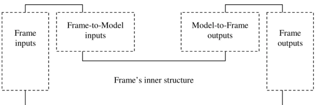
The frame’s formalization benefits from the DEVS hierarchy for systems specification. At each level of specification, more knowledge is revealed than at lower levels. One consequence of the dual relationship between models and frames is that each level of this hierarchy must produce at least a dual specification of any knowledge that was revealed for the model at the corresponding level of the model specification hierarchy. For this purpose, we adopt a systemic point of view, where the system to model is the whole problem under study, not only the source system. Then, a plug-in approach is used to separate the speci-fication of the source system from the specispeci-fication of the frame. With this approach, the lowest level of frame specification depicts the frame’s interface. The next level depicts the behavior expected within the frame. The last level details the frame’s inner structure. These specification levels provide a mean to get an operational formulation of at least the objectives, assumptions and constraints of the context.
3.1 Frame interface
Let us considering the whole problem to study as a system that aggregates the source system and the context of the study. If a model of such a system is conveniently built, it must necessarily involve a specification of the model of the source system, intermingled with a specification of the frame. The idea behind the plug-in approach is that we can infer the specification of the frame from the specification of the whole problem, by performing a kind of “model subtraction” like: frame = “model of the whole problem” – “model of the source system”. To picture this approach, one can represent the whole prob-lem as a circuit board built around a processor (i.e. the source system here), and then plug out the
pro-cessor. Then, the remaining card depicts the frame, which idle connectors indicates that inputs and out-puts are expected from a missing component.
It is noteworthy to mention that the inputs and outputs which are expected from the model, are also parts of the frame: the inputs for the model are a subset of the frame’s outputs, and the outputs for the model are a subset of the frame’s inputs. Indeed, these inputs and outputs form an interface to which must adhere both the model and the frame. The Generator-Acceptor-Transducer-based view presented in [23], which is made of a generator, an acceptor and a transducer, is nothing but a specific case of the type of frame that can be really built. A frame can be a more complex combination of components, which feed back each other eventually, and which in turn are coupled networks in their own right. Figure 2 illustrates the architecture of a frame as suggested by such an approach.
At the lower level of frame’s specification, we define the Frame Interface as a structure:
FI = <T, IM, IE, OM, OE>, where
T is a time base,
IM is the set of Frame-to-Model input variables, the plug-in input set,
IE is the set of Frame input variables, the control input set,
OM is the set of Model-to-Frame output variables, the plug-in output set,
OE is the set of Frame output variables, the summary set.
Frame’s inner structure Frame-to-Model inputs Frame inputs Frame outputs Model-to-Frame outputs
Figure 2. Frame interface 3.2 Frame behavior
What is expected to be done when a model is placed in some given circumstances? There is a need to specify the behavior of the corresponding frame. The DEVS specification hierarchy [25] provides two levels for specifying the functional behavior of a system : level 1 depicts the Input Output Relation Ob-servation (IORO), i.e. the timed-indexed IO pairs collected from the system, and level 2 depicts the In-put OutIn-put Function Observation (IOFO), i.e. the mapping of any inIn-put to a unique outIn-put depending on the state in which the system was when the input occurred. In the case of frame specification, the knowledge provided by the IORO level is meaningless, since the data pairs observed within a frame de-pend on the source system under observation. Indeed, the same context can be applied to different source systems, and also different contexts can be applied to the same source system. On the other hand, the IOFO knowledge is quite adequate to capture how the frame outputs are mapped to its inputs. This knowledge is based on the assumptions that the plugged model behaves as expected. Such assumptions could be characterized in terms of pre- and post-conditions.
At that stage of frame’s specification, we define a frame as a structure:
FB = <T, IM, IE, OM, OE, ΩM, ΩE, ΩC, SU>, where
ΩM is the set of admissible input segments for the plug-in component, the plug-in input
con-straints set (a subset of all time segments over the cross-product IM variables),
ΩE is the set of admissible input segments for the experimentation control, the plug-in input
con-straints set (a subset of all time segments over the cross-product of IE variables),
ΩC is the set of admissible output segments expected from the plug-in component, the plug-in
output constraints set (a subset of all time segments over the cross-product OM variables),
SU is the summary mapping, i.e. the set of pre- and post-conditions that maps the control input set to the summary set depending on the plug-in inputs and outputs.
While the frame interface specification tells us what criteria are focused, the frame behavior specifi-cation tells us how the final results of the study are obtained or what conditions should be verified to agree the use of a given model within the current context. This later specification can be used at a con-ceptual level for checking and reasoning, or be more detailed for implementation and coupling with software components.
3.3 Frame system
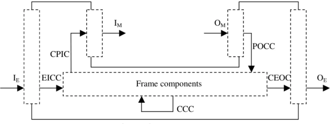
Level 3 and level 4 of the DEVS specification hierarchy bring more details to the structure and the be-havior of a system: level 3 gives the Input Output System (IOS), i.e. the state-to-state transition that governs the behavior of the system and the outputs that are generated by each state, and level 4 gives the Coupled Network (CN), i.e. the hierarchical decomposition of the system into coupled components. The plug-in approach that we have adopted implicitly suggests that we focus on the hierarchical decomposi-tion of a frame (CN level) rather than its atomic representadecomposi-tion (IOS level). Then, the third (and last lev-el) of frame specification characterizes the networked structure of a frame, as illustrated in figure 3.
We define a frame system as a structure:
FS = <T, IM, IE, OM, OE, ΩM, ΩE, ΩC, D, {Cd, d ∈ D}, CPIC, EICC, POCC, CEOC, CCC>,
where T, IM, IE, OM, OE, ΩM, ΩE, and ΩC are defined as above,
D is a set of component names, the control components set, Cd is a model for each d ∈ D,
CPIC is the Control-to-Plug-in-Input coupling {(d,j),(ES,i)) / i ∈ IM, d ∈ D, j ∈ Outputs(d)},
EICC is the External-Input-to-Control coupling {(ES,i),(d,j)) / i ∈ IE, d ∈ D, j ∈ Inputs(d)},
POCC is the Plug-in Output-to-Control coupling {(ES,i),(d,j)) / i ∈ OM, d ∈ D, j ∈ Inputs(d)},
CEOC is the Control-to-External-Output coupling {(d,j),(ES,i)) / i ∈ OE, d ∈ D, j ∈ Outputs(d)},
CCC is the Control-to-Control coupling {(d,i),(e,j)) / i ∈ Outputs(d), d ∈ D, e ∈ D, j ∈ In-puts(e)}. IE OE IM OM Frame components EICC CEOC CCC POCC CPIC
3.4 Abstract experimenters
The simulation relation presented in figure 2 plans for the building of an experimenter. We have previ-ously mentioned the cases where such a component is needed. An experimenter is for a frame what a simulator is for a model. In the DEVS framework, coupled models are assigned to coordinators and atomic models have their own simulators. All simulators and coordinators adhere to a generic message protocol that allows them to coordinate with each other to execute the simulation. Assignment of coor-dinators and simulators follows the lines of the hierarchical model structure, with simulators associated with the leaves of the hierarchical model, and coordinators assigned to the successive inner nodes of the hierarchy, until the top of the tree is reached, which is handled by a root coordinator in charge to initiate the simulation cycles. Abstract schemes have been defined in [25] to characterize what simulators and coordinators have to do.
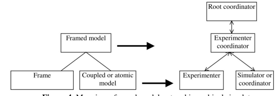
Let us introduce the concept of framed model as being the coupling between a model and a frame (i.e., the model resulting from adequately connecting the inputs and outputs of the model with the plug-in outputs and plug-plug-in plug-inputs of the frame). To map coherently this coupled model onto a hierarchical simulator, we map the model onto its own simulator and the frame onto its own experimenter, and an experimenter coordinator is used to coordinate the experimenter with the simulator. Moreover, the ex-perimenter adheres to the same generic message protocol. Figure 4 shows the principle of such a map-ping, which remains consistent since the experimenter coordinator is also a DEVS coordinator. Then, all coordinators, experimenters and simulators are indistinguishable from superior coordinators (due to space limitations, we do not present here the algorithms we have defined for the abstract experimenter and experimenter coordinator, both in discrete-event and discrete time cases).
Frame Coupled or atomic model Framed model Root coordinator Experimenter Simulator or coordinator Experimenter coordinator
Figure 4. Mapping a framed model onto a hierarchical simulator 4 APPLICATION
Here, the formal framework defined so far, is used in a fire spreading application. Fires are economical, ecological and human catastrophes. Especially as we know that present rising of wild land surfaces and climate warming will increase forest fires [13, 20]. Modeling such a huge and complex phenomenon ob-viously leads to simulation performances over design problems. To give real-time advice for fire fight-ers, fire spread simulators have to predict further fire spread positions quicker than the actual fire propa-gates. To improve the precision of current fire spread models, models from physics are currently used. However, the precision of these models make them difficult to be simulated under real-time constraints. Moreover, fire spread complexity requires increasing refinements of model specifications, depending on the simulation results. Thus, developing effective fire spread models remains a challenge for research.
Fire spread simulation is usually performed through cellular simulation models. To reduce execution times of these models, a new method called Dynamic Structure Cellular Automata (DSCA) [3, 14], based on modeling formalisms for dynamic structure systems [4], has been recently designed. While tra-ditional Cellular Automata (CA) compute even non active cells, DSCA only concentrate the simulation on the active ones. We compare here execution times of both DSCA and CA Fire Spread Models (FSM) against actual fire propagation times. Moreover, outputs of both models are guaranteed to be the same thanks to an error calculation. The Fire Spread Experimental Frame (FSEF) used to specify influences of both fire spread simulation models allows us to achieve these comparisons, as well as to improve the modeling process.
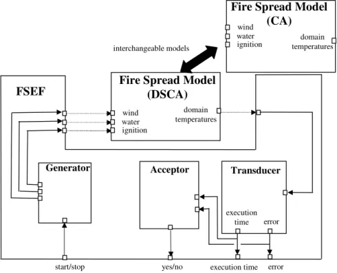
4.1 Fire Spread Study Model
Figure 5 sketches the Fire Spread Study Model (FSSM). Both CA and DSCA hold four ports: the “wa-ter”, “wind” and “ignition” input ports (for the external events able to affect fire spreading) and the “domain temperatures” output port. The FSEF interacts with the FSM through these ports, using a gen-erator to simulate external events, and a transducer to convert the output domain temperatures to be dis-played. Also, according to the execution time of the model under test, an acceptor validates or invali-dates the simulation by sending a Boolean value on its “yes/no” output port. Both CA and DSCA can be easily interchanged in the FSSM.
Generator Acceptor Transducer
yes/no start/stop FSEF domain temperatures wind
Fire Spread Model (DSCA)
domain temperatures Fire Spread Model
(CA) interchangeable models execution time execution time error error water ignition wind water ignition
Figure 5. Fire Spread Study Model 4.2 Fire Spread Models
We use the mathematical fire spread model already validated and presented in [1]. In this model, a Par-tial DifferenPar-tial Equation (PDE) represents the temperature of each cell. A CA is obtained after discre-tizing the PDE. Using the finite difference method leads to the following algebraic equation:
k j i dT ig t t e v c k j i T k j i T b k j i T k j i T a k j i T,+1= ( −1, + +1, )+ ( , −1+ , +1)+ σ ,0 −α(− )+ ,
where Tij is the grid node temperature. The coefficients a, b, c and d depend on the time step and mesh
size considered, t is the real time, tigthe real ignition time (the time the cell is ignited) and σν,0 is the
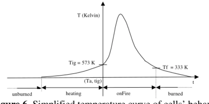
ini-tial combustible mass. Figure 6 depicts a simplified temperature curve of a cell in the domain. We con-sider that above a threshold temperature Tig the combustion occurs and below a Tf temperature the
com-bustion is finished. The end of the real curve is purposely neglected to save simulation time. Four states corresponding to each cell’s behavior are defined from these assumptions. A cell has states “unburned”, “heating”, “onFire” and “burned”. More details and specifications of both CA and DSCA are provided in [14]. A corresponding simulator is presented in [15].
t (Ta, tig)
Tf = 333 K Tig = 573 K
T (Kelvin)
heating onFire burned unburned
Figure 6. Simplified temperature curve of cells’ behavior 4.3 Fire Spread Experimental Frame specification
We give hereafter, the complete specification of the FSEF, using the formal framework in a context of experimentation. Then, an experimenter has been built for the frame which structure is described above:
FSEF = <T, IM, IE, OM, OE, ΩM, ΩE, ΩC, D, {Cd, d ∈ D}, CPIC, EICC, POCC, CEOC, CCC>, where:
T = ℵ,
IM = {wind, water, ignition},
IE = {start/stop},
OM = {domain temperatures},
OE = {execution time, error}, where
error indicates the average error between the CA and DSCA output domain temperatures,
ΩM = {(w,t) / t ∈ <tinit,tend>}, with
w ∈ {( data type, data value, cell coordinates)}
ΩE = {(start, tinit),(stop, tend)},
ΩC = { error < ε, texecution< treal propagation}, where
ε is a threshold under which the simulation can be accepted, texecution indicates the execution time, and
treal propagation indicates the actual fire propagation times,
D = {Gen, Trans, Acc},
CPIC= {((Gen, data), (FSEF, data))}
EICC = {((FSEF, start/stop), (Gen, start/stop))}
CEOC = {((Trans, execution time), (FSEF, execution time)), ((Trans, error), (FSEF, error)), ((Acc, yes/no), (FSEF, yes/no))}
CCC = {((Gen, data), (Trans, data)), ((Trans, execution time), (Acc, execution time)), ((Trans, er-ror), (Acc, error))}
Gen, Trans and Acc are DTSS atomic models [25], i.e., structures: Cd = <Xd, Qd, Yd, δd, λd>, where Xd is
the set of input values, Yd is the set of output values, Qd is the set of states, δd : Qd×Xd Qd is the
tran-sition function, and λd : Qd Yd is the output function. 4.4 Simulation process
The whole simulation is performed using a discrete time basis. This means that at every time step of the simulation, transition and output functions of the atomic models of the FSSM are activated. A Simula-tion is started by sending a “start” message on the start/stop port of the generator. Receiving this event, the Generator’s transition function δG changes the model’s phase to “active” and sends a first ignition to
the model. At each time step, the Transducer’s transition function δT saves the “domain temperatures”
and calculates the error using the output file of the previously simulated model, when available (e.g. the DSCA FSM if the CA model is being simulated). The simulation time “tsim” is then compared to the
simulation time “tend” corresponding to the end of the simulation. When the simulation ends, the
transi-tion functransi-tion δT saves the execution time “texecution”, and the output function λT sends two messages to
the Acceptor and the FSEF. One of them contains the error result, and is sent through the “error” port. The other one contains the total execution time, and is sent though the “execution time” port. The Ac-ceptor is devoted to check the values received on its ports at each time step. If the “error” is greater than a certain threshold ε defined by the user, or if the total execution time “texecution” is greater than the
actu-al fire propagation time “treal propagation”, the “yes/no” value takes a value “no” to invalidate the
simula-tion.
4.5 Results
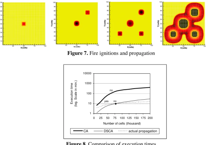
During fire spreading, flying brands ignite new unburned parts of land away from the fire. This is an im-portant cause of fire spreading. Figure 7 represents a case of multi-ignitions during the simulation. Both outputs of the DSCA and CA FSM are the same. Simulation starts with one ignition on the center of the propagation domain. Then, at time t=7s, a second ignition occurs on the top right corner of the propaga-tion domain. Finally, at t=12s, two new ignipropaga-tions occur on the right and left bottom of the propagapropaga-tion domain. Last picture shows the multiple fire fronts positions at t=70s.
Figure 8 compares execution times of both DSCA and CA Fire Spread Models, against actual fire propagation times. Simulations have been performed using a 500 MHz Pentium III processor. Validation and invalidation results of the FSEF’s Acceptor are written as “yes” and “no” on the curves. CA execu-tion times are definitely too long to give real-time advice for fire fighters. DSCA ones are valid up to 75 thousand cells. Above this threshold, DSCA simulation is invalidated too by the FSEF’s Acceptor.
Keeping the same FSEF, both DSCA and CA FSM can be easily tested by looking at the Acceptor’s output value at the end of the simulations. Both models provide the same fire front positions, but the CA never meets the real time deadline requirements. For a high number of cells, the DSCA simulation has been invalidated too. However, for very high number of cells, parallel simulation techniques using this well optimized simulation already provided promising results [11].
The greatest advantage in using the formal framework relates to the clarity of model definitions and specifications. The FSEF definition guided us to specify what is intrinsic to the FSM and what is exter-nal to these models. Moreover, using the specification of FSEF has undoubtedly reduced development and testing times, even if no quantitative measures are available to attest this fact. Reusability has also been improved, since the FSEF can be reused to test other fire spread models. Also, various other frames can be defined to study various FSM properties (e.g. accuracy, reliability, etc.).
Figure 7. Fire ignitions and propagation
1 10 100 1000 10000 0 25 50 75 100 125 150 175 200
Number of cells (thousand)
E x e c u ti o n t im e (l o g . S c a le i n m in .)
CA DSCA actual propagation
yes no no
Figure 8. Comparison of execution times 5 DISCUSSION
This application has shown a contribution in describing the use of an experimental frame to the dynam-ics of fire spread. However, the formal framework can extend to other applications. To a great extent, the idea of frame can even be used to catch the structure and the behavior of a model that has more than one abstraction layer. In this case, a lower abstraction layer can be seen as a model which context is de-fined in the next higher abstraction layer. Such a case often appears in business work flow simulation [10, 21], where a business process flow is modeled as entities moving within and among organizations, and business processes are the activities of an organization. This usually leads to a hierarchical model describing the business process network at the top level, and underlying business processes (at lower levels) which, in turns, may also be modeled to express local area details. The frame concept can be used to model the process of running a business process, as well as to model the process of executing the en-tire work flow. Also, distributed systems often exhibit situations where there is a need to model a model that includes multiple abstraction layers, especially when human decision making are involved. The frame can be defined as modeling the process of inferring decisions from the execution of a model that
X(cells) Y (c e ll s ) 25 50 75 100 10 20 30 40 50 60 70 80 90 100 X(cells) Y (c e ll s ) 25 50 75 100 10 20 30 40 50 60 70 80 90 100 X(cells) Y (c e ll s ) 25 50 75 100 10 20 30 40 50 60 70 80 90 100 X(cells) Y (c e ll s ) 25 50 75 100 10 20 30 40 50 60 70 80 90 100
represents the underlying resource used by a decision maker (e.g, endomorphic agent [24]), while also being used to catch the whole context in which the distributed system is studied.
An important issue linked to this formal framework is the applicability of frames to models. It relates to the legitimacy of coupling a model with a frame. A natural way to do such a coupling is to consider pairs of specifications at equivalent levels of specification, as suggested by figure 9. An applicability re-lationship holding between a frame and a model that are specified at equivalent levels, must imply the same thing at lower levels. The theoretical aspects of applicability (and derivability) have been intro-duced in [25]. The formal framework proposed here concretizes its operational aspects.
Input/Output Relation Observation
Frame behavior Frame system
Frame interface
Model specification Frame specification
applicability mapping Frame behavior Frame system Frame interface derivability
Input/Output Function Observation
Observation Frame Input/Output System
Coupled Network
Figure 9. Specification hierarchies for models and frames, and their relationships 6 CONCLUSION
By formalizing frames, we have defined a basis for specifying the context in which simulation models are built or called up. Extending the principle of separation of concerns to the context level, we have de-fined a formal framework for capturing the model-context duality, then opening the way to specification and symbolic manipulation of some fundamental concepts of the M&S process. Hence, we can enhance our understanding of these concepts and then improve our approach to model building and verification. This formal framework has been used in a fire spreading application. It has shown that the development and the testing processes are facilitated, and that the specifications are improved with regard to clarity and manipulability.
The plug-in-based view does not formally forbid the specification of a frame in the shape of an atomic model. We suggest such a specification be obtained by the counterpart specification of the frame structure at the IOS level. This excludes from our work the case of non decomposable frames.
The next step in this work is the integration of formal methods for the specification of models and frames (especially at the frame behavior specification level), so as to allow formal verification of models consistency, models composability and reuse, and models validity, by the means of model checkers and theorem provers.
ACKNOWLEDGEMENTS
This work was initiated by a research collaboration with Bernard Zeigler. Most of the ideas presented here stem from his scientific leading. One of the authors would specially like to thank the participants of the 2004 Dagstuhl seminar on Component-based Modeling and Simulation, for helpful discussions. Spe-cial thanks to Thomas Santen, Alexander Verbraeck, and Gabriel Wainer.
REFERENCES
[1] Balbi, J. H., P. A. Santoni, and J. L. Dupuy. 1998. Dynamic Modelling of Fire Spread Across a Fuel Bed. International Journal of Wildland Fire. 275-284.
[2] Balci, O. 1998. Verification, Validation, and Accreditation. Proceedings of the 1998 Winter
Sim-ulation Conference. D.J. Medeiros, E.F. Watson, J.S. Carson and M.S. Manivannan (eds). 42-48. [3] Barros, F.J., and M.T. Mendes. 1997. Fire Modelling in the DELTA Simulation Environment.
Simulation Practice and Theory 5. 185-197.
[4] Barros, F.J. 1997. Modelling Formalisms for Dynamic Structure Systems. ACM Transactions on
Modelling and Computer Simulation 7 (4). 501-515.
[5] Clarke, E.M., and J.M. Wing. 1996. Formal Methods: State of the Art and Future Directions.
ACM Computing Surveys, 28 (4). 626-643.
[6] Dagstuhl Seminar, 2002. Grand Challenges for Modeling and Simulation, Dagstuhl Report, R. M. Fujimoto, D. Lunceford, E. Page, and A. Uhrmacher (eds). Available online via
<http://www.informatik.uni-rostock.de/%7Elin/GC/report/Dagstuhl_Report.pdf> [accessed April
22, 2004].
[7] Daum, T., and R. Sargent. 2001. Experimental Frames in a Modern Modeling and Simulation System. IIE Transactions 33 (3), 181-192.
[8] Davis, P.K., and R.H. Anderson. 2003. Improving the Composability of Department of Defense Models and Simulations. RAND Corporation.
[9] Fishwick, P. 1995. Simulation Model Design and Execution. Building Digital Worlds. Prentice Hall, Englewood Cliffs, NJ.
[10] Hlupic, V., and S. Robinson. 1998. Business Process Modelling and Analysis Using Discrete-Event Simulation. Proceedings of the 30th Winter Simulation. 1363-1369.
[11] Innocenti, E., A. Muzy, A. Aïello, J.F. Santucci, and D.R.C. Hill. 2003. Design of a Multithread-ed Parallel Model for Fire Spread. ProceMultithread-edings of the 15th European Simulation Symposium. 104-109.
[12] Mayer, R., and R.E. Young. 1984. Automation of Simulation Model Generation From System Specifications. Proceedings of the 16th Winter Simulation Conference. 570-574.
[13] McKenzie, D., Z. Geladof, D.L. Peterson, and P. Mote. 2004. Climatic Change, Wildfire and Conservation. Conservation Biology 18 (4). 890-902.
[14] Muzy, A., E. Innocenti, D.R.C. Hill, A. Aïello, J.F. Santucci, and P.A. Santoni. 2004. Dynamic Structure Cellular Automata in a Fire Spreading Application. Proceedings of the First
Interna-tional Conference on Informatics in Control, Automation and Robotics, IEEE/CSS/IFAC/ACM/AAAI/APPIA, Setubal, Portugal, to be published.
[15] Muzy, A., E. Innocenti, F. Barros, A. Aïello, et J. F. Santucci. 2003. Efficient Simulation of Large-scale Dynamic Structure Cell Spaces. Proceedings of SCSC’03, Montréal. 378-383. [16] Nance, R. E. 1994. The Conical Methodology and the Evolution of Simulation Model
[17] Overstreet, C. M., R. E. Nance, and O. Balci. 2002. Issues in Enhancing Model Reuse.
Interna-tional Conference on Grand Challenges for Modeling and Simulation, Jan. 27-31, San Antonio, Texas, USA.
[18] Traoré, M.K. 2004. Conditions for Model Component Reuse. Dagstuhl Seminar, 2004.
Compo-nent-based Modeling and Simulation, Dagstuhl Report, F.J. Barros, A. Lehmann, P. Liggesmey-er, A. Verbraeck, B.P. Zeigler (eds), January 18-23. Available online via <http://www.dagstuhl.de/04041/Talks/> [accessed April 22, 2004].
[19] Traoré, M.K. 2003. Experimental Frames Methodology. NSF Workshop on Modeling and
Simu-lation for Design of Large Software-Intensive Systems: Challenges and New Research Directions (M&Snet meeting), Tucson (AZ), December 11-13. Available online via
<http://www.site.uottawa.ca/~oren/SCS_MSNet/pres/pres-list.htm> [accessed April 22, 2004].
[20] Torn, M.S., and J.S. Fried. 1992. Predicting the Impacts of Global Warming on Wildland Fire.
Climatic Change 21 (3). 257-274.
[21] Weyland, J.H., and
M.http://portal.acm.org/results.cfm?query=author%3AP246979&querydisp=author%3ARobert%
20E%2E%20Young&coll=portal&dl=ACM&CFID=20421726&CFTOKEN=37995320 Engiles.
2003. Towards Simulation-Based Business Process Management. Proceedings of the 35th Winter
Simulation Conference. 225-227.
[22] Zeigler B. P. 1976. Theory of Modelling and Simulation. Wiley & Sons, N.Y.
[23] Zeigler, B. P. 1984. Multifacetted Modelling and Discrete Event Simulation. Academic Press Inc., London.
[24] Zeigler, B.P. 1990.Object Oriented Simulation with Hierarchical, Modular Models: Intelligent Agents and Endomorphic Systems. Academic Press.
[25] Zeigler, B. P., H. Praehofer, and T. G. Kim. 2000. Theory of Modeling and Simulation. Integrat-ing Discrete Event and Continuous Complex Dynamic Systems. 2nd Edition. Academic Press.