Depth from motion algorithm and hardware architecture for smart cameras

HAL Id: hal-01964830

https://hal.archives-ouvertes.fr/hal-01964830

Submitted on 23 Dec 2018

HAL is a multi-disciplinary open access

archive for the deposit and dissemination of

sci-entific research documents, whether they are

pub-lished or not. The documents may come from

teaching and research institutions in France or

abroad, or from public or private research centers.

L’archive ouverte pluridisciplinaire HAL, est

destinée au dépôt et à la diffusion de documents

scientifiques de niveau recherche, publiés ou non,

émanant des établissements d’enseignement et de

recherche français ou étrangers, des laboratoires

publics ou privés.

for smart cameras

Abiel Aguilar-González, Miguel Arias-Estrada, François Berry

To cite this version:

Abiel Aguilar-González, Miguel Arias-Estrada, François Berry. Depth from motion algorithm and

hardware architecture for smart cameras. Sensors, MDPI, 2018. �hal-01964830�

Depth from motion algorithm and hardware

architecture for smart cameras

Abiel Aguilar-González1,2* , Miguel Arias-Estrada1and François Berry2, 1 _{Instituto Nacional de Astrofísica, Óptica y Electrónica (INAOE), Tonantzintla, Mexico} 2 _{Institut Pascal, Université Clermont Auvergne (UCA), Clermont-Ferrand, France} * Correspondence: abiel@inaoep.mx, abiel.aguilar_gonzalez@etu.uca.fr

Academic Editor: name

Version November 26, 2018 submitted to Sensors

Abstract:Applications such as autonomous navigation, robot vision, autonomous flying, etc., require 1

depth map information of the scene. Depth can be estimated by using a single moving camera 2

(depth from motion). However, traditional depth from motion algorithms have low processing speed 3

and high hardware requirements that limits the embedded capabilities. In this work, we propose 4

a hardware architecture for depth from motion that consists of a flow/depth transformation and 5

a new optical flow algorithm. Our optical flow formulation consists in an extension of the stereo 6

matching problem. A pixel-parallel/window-parallel approach where a correlation function based in 7

the Sum of Absolute Differences computes the optical flow is proposed. Further, in order to improve 8

the Sum of Absolute Differences performance, the curl of the intensity gradient as preprocessing step 9

is proposed. Experimental results demonstrated that it is possible to reach higher accuracy (90% of 10

accuracy) compared with previous FPGA-based optical flow algorithms. For the depth estimation, 11

our algorithm delivers dense maps with motion and depth information on all the image pixels, with 12

a processing speed up to 128 times faster than previous works and making it possible to achieve high 13

performance in the context of embedded applications. 14

Keywords:Depth estimation; monocular systems; optical flow; smart cameras; FPGA 15

1. Introduction 16

Smart cameras are machine vision systems which, in addition to image capture circuitry, are 17

capable of extracting application-specific information from the captured images. For example, for 18

video surveillance, image processing algorithms implemented inside the camera fabric could detect 19

and track pedestrians [1], but for a robotic application, computer vision algorithms could estimate 20

the system egomotion [2]. In recent years, advances in embedded vision systems such as progress in 21

microprocessor power and FPGA technology allowed the creation of compact smart cameras with 22

increased performance for real world applications [3–6]. As result, in current embedded applications, 23

image processing algorithms inside the smart cameras fabric deliver an efficient on-board solution 24

for: motion detection [7], object detection/tracking [8,9], inspection and surveillance [10], human 25

behavior recognition [11], etc. Another algorithm that could be highly used by smart cameras are 26

computer vision algorithms since they are the basis of several applications (automatic inspection, 27

controlling processes, detecting events, modeling objects or environments, navigation and so on). 28

Unfortunately, mathematical formulation of computer vision algorithms is not compliant with the 29

hardware technologies (FPGA/CUDA) often used in smart cameras. In this work, we are interested 30

in depth estimation from monocular sequences in the context of a smart camera because depth is the 31

basis to obtain useful scene abstractions, for example: 3D reconstructions of the world and the camera 32

egomotion. 33

1.1. Depth estimation from monocular sequences 34

In several applications, like autonomous navigation [12], robot vision and surveillance [1], 35

autonomous flying [13], etc., there is a need for determining the depth map of the scene. Depth 36

can be estimated by using stereo cameras [14], by changing focal length [15], or by employing a single 37

moving camera [16]. In this work we are interested in depth estimation from monocular sequences 38

by using a single moving camera (depth from motion). This choice is motivated because monocular 39

systems have higher efficiency compared with other approaches, simpler and more accurate than 40

defocus techniques and, cheaper/smaller compared with stereo-based techniques. In monocular 41

systems, depth information can be estimated based on two or multiple frames of a video sequence. For 42

two frames, image information may not provide sufficient information for accurate depth estimation. 43

The use of multiple frames improves the accuracy, reduces the influence of noise and allows the 44

extraction of additional information which cannot be recovered from just two frames, but the system 45

complexity and computational cost is increased. In this work, we use information from two consecutive 46

frames of the monocular sequence since our algorithm is focused for smart cameras and in this context 47

hardware resources are limited. 48

1.2. Motivation and scope 49

In the last decade several works have demonstrated that depth information is highly useful for 50

embedded robotic applications [1,12,13]. Unfortunately, depth information estimation is a relatively 51

complex task. In recent years, the most popular solution is the use of active vision to estimate depth 52

information from the scene [17–21], i.e., LIDAR sensors or RGBD cameras that can deliver accurate 53

depth maps in real time, however they increase the systems size and cost. In this work, we propose 54

a new algorithm and an FPGA hardware architecture for depth estimation. First, a new optical 55

flow algorithm estimates the motion (flow) at each point in the input image. Then, a flow/depth 56

transformation computes the depth in the scene. For the optical flow algorithm: an extension of the 57

stereo matching problem is proposed. A pixel-parallel/window-parallel approach where a Sum of 58

Absolute Differences computes the optical flow is implemented. Further, in order to improve the Sum 59

of Absolute Differences performance, we propose the curl of the intensity gradient as preprocessing 60

step. For the depth estimation proposes: we introduce a flow/depth transformation inspired in the 61

epipolar geometry. 62

2. Related work 63

In previous works, depth estimation is often estimated by using a single moving camera. This 64

approach is called depth from motion and consists in computing the depth from the pixel velocities 65

inside the scene (optical flow). i.e., optical flow is the basis for depth from motion. 66

2.1. FPGA architectures for optical flow 67

In [22], a hardware implementation of a high complexity algorithm to estimate the optical 68

flow from image sequences in real time is presented. In order to fulfil with the architectural 69

limitations, the original gradient-based optical flow was modified (using a smoothness constraint for 70

decreasing iterations). The developed architecture can estimate the optical flow in real time and can be 71

constructed with FPGA or ASIC devices. However, due to the mathematical limitations of the CPU 72

formulation (complex/iterative operations), speed processing is low, compared with other FPGA-based 73

architectures for real-time image processing [23,24]. In [25], a pipelined optical-flow processing system 74

that works as a virtual motion sensor is described. The proposed approach consists of several spatial 75

and temporal filters (Gaussian and gradient spatial filters and IIR temporal filter) implemented in 76

cascade. The proposed algorithm was implemented in an FPGA device, enabling the easy change 77

of the configuration parameters to adapt the sensor to different speeds, light conditions and other 78

environmental factors. This makes possible the implementation of an FPGA-based smart camera for 79

optical flow. In general, the proposed architecture reaches a reasonable hardware resources usage 80

but accuracy and processing speed is low (lower than 7 fps for 640×480 image resolution). In [26], a 81

tensor-based optical flow algorithm is presented. This algorithm was developed and implemented 82

using FPGA technology. Experimental results demonstrated high accuracy compared with previously 83

FPGA-based algorithms for optical flow. In addition, the proposed design can process 640×480 images 84

at 64 fps with a relatively low resource requirement, making it easier to fit into small embedded 85

systems. In [27], a highly parallel architecture for motion estimation is presented. The developed 86

FPGA-architecture implements the Lucas and Kanade algorithm [28] with the multi-scale extension for 87

the computation of large motion estimations in an FPGA. Although the proposed architecture reaches 88

a low hardware requirement with a high processing speed, the use of huge external memory capacity 89

is needed. Further, in order to fulfil with the hardware limitations, the accuracy is low (near 11% more 90

error compared with the original CPU version of the Lukas and Kanade algorithm). Finally, in [29], 91

an FPGA-based platform with the capability of calculating real-time optical flow at 127 frames per 92

second for a 376×240 pixel resolution is presented. Radial undistortion, image rectification, disparity 93

estimation and optical flow calculation tasks are performed on a single FPGA without the need of 94

external memory. So, the platform is perfectly suited for mobile robots or embedded applications. 95

Unfortunately, accuracy is low (qualitatively lower accuracy than CPU based approaches). 96

2.2. Optical flow methods based in learning techniques 97

There are some recent works that addresses the optical flow problem via learning techniques [30]. 98

In 2015 [31] proposed the use of convolutional neuronal networks (CNNs) as an alternative framework 99

to solve the optical flow estimation problem. Two different architectures were proposed and compared: 100

a generic architecture and another one including a layer that correlates feature vectors at different 101

image locations. Experimental results demonstrated a competitive accuracy at frame rates of 5 to 102

10 fps. On the other hand, in 2017 [32] developed a stacked architecture that includes warping of 103

the search image with intermediate optical flow. Further, in order to achieve high accuracy on small 104

displacements, authors introduced a sub-network specializing on small motions. Experimental results 105

demonstrated that it is possible to reach more than 95% of accuracy, decreasing the estimation error by 106

more than 50% compared with previous works. 107

3. The proposed algorithm 108

In Fig.1an overview of our algorithm is shown. First, given an imager as sensor, two consecutive 109

frames(ft(x, y), ft+1(x, y))are stored in local memory. Then, an optical flow algorithm computes 2D

110

pixel displacements between ft(x, y)and ft+1(x, y). A dynamic template based on the optical flow

111

previously computed(∆_x,t−1(x, y), ∆y,t−1(x, y))computes the search region size for the current optical

112

flow. Then, let the optical flow for the current frame be(∆x(x, y), ∆y(x, y)), the final step is depth

113

estimation for all the pixels in the reference image D(x, y). In the following subsections, details about 114

the proposed algorithm are presented. 115

3.1. Frame buffer 116

The first step in our mathematical formulation is image storage, considering that in most cases the 117

imager provides data as a stream, some storage is required in order to have two consecutive frames 118

available at the same time t. More information/details about the storage architecture are presented 119

in Section4.1. For mathematical formulation, we consider the first frame (frame at t time) as ft(x, y)

120

while the second frame (frame at t+1 time) is ft+1(x, y).

121

3.2. Optical flow 122

In previous works, iterative algorithms, such as the Lucas Kanade [28] or the Horn–Schunck [33] 123

algorithms have been used on order to compute optical flow across video sequences, then, given dense 124

optical flow, geometric methods allow to compute the depth in the scene. However, these algorithms 125

[28,33] have iterative operations that limit the performance for smart camera implementations. In 126

order to avoid the iterative and convergence part of the traditional formulation we replace that with a 127

correlation metric implemented inside a pixel-parallel/window-parallel formulation. In Fig.2an 128

overview of our optical flow algorithm is shown. Let(ft(x, y), ft+1(x, y)be two consecutive frames

129

from a videosequence, curl of the intensity gradient d f (x,y)_dx are computed, see Eq.1, where∇is 130

the Del operator. Let curl be a vector operator that describes the infinitesimal rotation, then, at 131

every pixel the curl of that pixel is represented by a vector where attributes (length and direction) 132

characterize the rotation at that point. In our case, we use only the norm of Curl(x, y), as shown in 133

Eq.2and, as illustrated in Fig.3. This operation increases the robustness under image degradations 134

(color/texture repetition, illumination changes, noise), therefore, simple similarity metrics [34] deliver 135

accurate pixel tracking, simpler than previous tracking algorithms [28,33]. Given the curl images for 136

two consecutive frames(Curlt(x, y), Curlt+1(x, y), dense optical flow(∆x(x, y), ∆y(x, y), illustrated 137

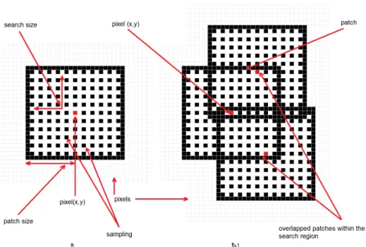
in Fig. 4)in the reference image is computed as shown in Fig. 5. This process assumes that pixel 138

displacements between frames is such as it exists an overlap on two successive "search regions". A 139

search region is defined as a patch around a pixel to track. Considering that between ftand ft+1, the

140

image degradation is low, any similarity-based metric have to provide good accuracy. In our case, this 141

similarity is calculated by a SAD (Sum of Absolute Difference). This process is defined in Eq.3; where 142

r is the patch size (see Fig.5).(Curlt(x, y), Curlt+1(x, y))are curl images on two consecutive frames.

143

x, y are the spatial coordinates of pixels in ftand, a, b are the spatial coordinates within a search region

144

constructed in ft+1(see Eq.4and5); where∆0_x(t−1),∆0_y(t−1)are a dynamic search template, computed

145

as shown in Section3.3. k is the search size and s is a sampling value defined by the user. Finally, 146

optical flowat the current time(∆x(x, y), ∆y(x, y))is computed by Eq.6.

147

148

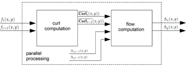
Figure 2.The optical flow step: first, curl images(Curlt(x, y)),(Curlt+1(x, y))are computed. Then, given the curl images for two consecutive frames, pixels displacements∆x(x, y),∆y(x, y)(optical flow for all pixels in the reference image) are computed using a dynamic template based on the optical flow previously computed(∆_x,t−1(x, y), ∆_y,t−1(x, y)).

(a) input(f(x, y)) (b) output Curl(x, y)

Figure 3.Curl computation example. Input image taken from the KITTI benchmark dataset [35]

(a)∆x(x, y) (b)∆y(x, y))

Figure 4.Optical flow example. Image codification as proposed in the Tsukuba benchmark dataset [36]

Curl(x, y) = ∇ ×d f(x, y) dx = ∂ ∂y ∂ f(x, y) ∂x − ∂ ∂x ∂ f(x, y) ∂y (1) Curl(x, y) = |∂ ∂y ∂ f(x, y) ∂x − ∂ ∂x ∂ f(x, y) ∂y | (2) where 149 ∂ f(x, y) ∂x =Gx(x, y) = f(x+1, y) −f(x−1, y) ∂ f(x, y) ∂y =Gy(x, y) = f(x, y+1) −f(x, y−1) ∂ ∂y ∂ f(x, y) ∂x =Gx(x, y+1) −Gx(x, y−1) ∂ ∂x ∂ f(x, y) ∂y =Gy(x+1, y) −Gy(x−1, y) 150 SAD(a, b) = u=r

∑

∑

Figure 5.The proposed optical flow algorithm formulation: patch size = 10, search size = 10, sampling value = 2. For each pixel in the reference image ft, n overlapped regions are constructed in ft+1, n region center that minimizes or maximizes any similarity metric is the tracked position (flow) of the pixel(x, y)at ft+1.

3.3. Search template 151

In optical flow, the search window size defines the maximum allowed motion to be detected in the 152

sequence, see Fig.4. In general, let p be a pixel in the reference image(ft), whose 2D spatial location is

153

defined as(xt, yt), the same pixel in the tracked image(ft+1)has to satisfy xt+1 ∈xt−k : 1 : x+k,

154

yt+1∈y−k : 1 : yt+k, where k is the search size for the tracking step. In practice, large search region

155

sizes increase the tracking performance since feature tracking could be carried out in both slow and 156

fast camera movements. However, large search sizes decrease the accuracy, i.e., if the search region size 157

is equal to 1, then, xt+1∈xt−1 : 1 : xt+1, yt+1∈yt−1 : 1 : yt+1 so, there are 9 possible candidates

158

for the tracking step and the mistake possibility is equal to 8, this considering that camera movement 159

is slow and therefore pixel displacements between images are close to cero. In other scenario, if the 160

search region size is equal to 10, then, xt+1∈xt−10 : 1 : xt+10, yt+1∈yt−10 : 1 : yt+10 so, there

161

are 100 possible candidates for the tracking step and the mistake possibility is equal to 99. In our 162

work, we propose to use the feedback of the previous optical flow step as a dynamic search size for 163

the current step so, if camera movement in t−1 is slow, small search sizes closer to the pixels being 164

tracked(xt, yt)are used. On the other hand, given fast camera movements small search sizes far to

165

the pixels being tracked are used. This makes the tracking step compute accurate results without 166

outliers, furthermore, the use of small search sizes decreases the computational resources usage. For 167

practical purposes we use a search region size equal to 10 since it provides a good tradeoff between 168

robustness/accuracy and computational resources. So, let∆x,t−1(x, y), ∆y,t−1(x, y)be the optical flow

169

at time t−1, the search template for the current time is computed as shown in Eq.7-8, where k is the 170 template size. 171 ∆0 x(x+u, y+v) = u=k,v=k

∑

∑

∆0 y(x+u, y+v) = u=k,v=k

∑

∑

In previous works it was demonstrated that monocular image sequences provide only partial 173

information about the scene due to the computation of relative depth, unknown scale factor, etc. [37]. 174

In order to recover the depth in the scene it is necessary to have assumptions about the scene and its 175

2-D images. In this work we assume that environment within the scene is rigid, then, given the optical 176

flow of the scene (which represents pixel velocity across time), we suppose that depth in the scene is 177

proportional to the pixel velocity. i.e., far objects have to be associated with a low velocity value while 178

closer objects are associated with high velocity values. This could be considered as an extension of the 179

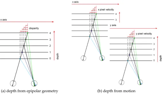
epipolar geometry in which disparities values are proportional with the depth in the scene, as shown 180

in Fig.6. 181

(a) depth from epipolar geometry (b) depth from motion

Figure 6. (a) Epipolar geometry: depth in the scene is proportional to the disparity value, i.e., far objects have low disparity values while closer objects are associated with high disparity values. To compute the disparity map (disparities for all pixels in the image) a stereo pair (two images with epipolar geometry) are needed. (b) Single moving camera: in this work we suppose that depth in the scene is proportional to the pixel velocity across the time. To compute the pixel velocity, optical flow across two consecutive frames has to be computed.

So, let∆x(x, y),∆y(x, y)be the optical flow (pixel velocity) at t time, depth in the scene depth(x, y)

182

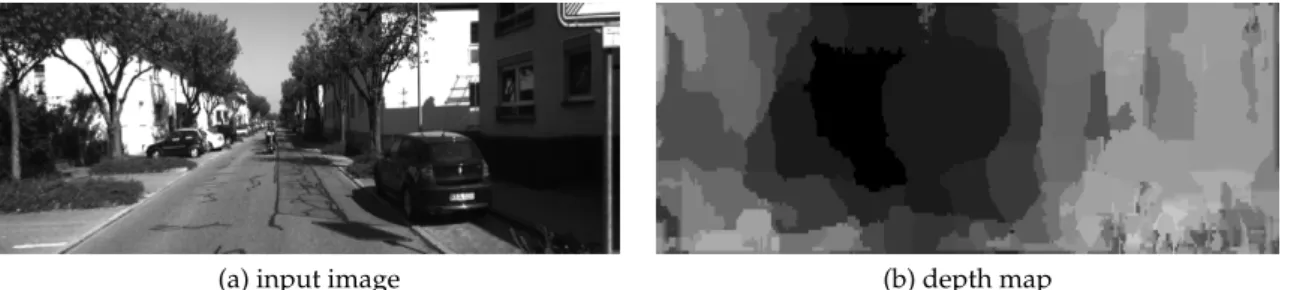
is computed as proposed in Eq. 9, where depth(x, y)is the norm of the optical flow. In Fig. 7an 183

example of depth map computed by the proposed approach is shown. 184

depth(x, y) = ||[∆x(x, y),∆y(x, y)]|| =

q

(a) input image (b) depth map Figure 7.Depth estimation using the proposed algorithm 4. The FPGA architecture

185

In Fig. 8, an overview of the FPGA architecture for the proposed algorithm is shown. The 186

architecture is centered on an FPGA implementation where all recursive/parallelizable operations 187

are accelerated in the FPGA fabric. First, the "frame buffer" unit reads the pixel stream (pix [7:0]) 188

delivered by the imager. In this block, frames captured by the imager are feed to/from an external 189

DRAM memory and delivers pixel streams for two consecutive frames in parallel (pix1 [7:0], pix2 [7:0]). 190

"Circular buffers" implemented inside the "Optical flow" unit are used to hold local sections of the 191

frames that are beingprocessedand allow for local parallel access that facilitates parallel processing. 192

Finally, optical flow streams (pix3 [7:0], pix4 [7:0]) are used to computed the depth in the scene (pix7 193

[7:0]). In order to hold optical flow previously computed (which are used for the dynamic search 194

template computation) a second "frame buffer" is used. In the following subsections details about the 195

algorithm parallelization are shown. 196

Figure 8.FPGA architecture for the proposed algorithm 4.1. Frame buffer

197

Images from the image sensor are stored in an external DRAM that holds an entire frame from the 198

sequence, and later the DRAM data is read by the FPGA to cache pixel flow of the stored frame into 199

circular buffers. In order to deliver two consecutive frames in parallel two DRAM chips in switching 200

mode are used. i.e.: 201

1. t1: DRAM 1 in write mode (storing frame 1), DRAM 2 in read mode (invalid values), frame 1 at

202

output 1, invalid values at output 2. 203

2. t2: DRAM 1 in read mode (reading frame 1), DRAM 2 inwritemode (storing frame 1), frame 1 at

204

output 2, frame 1 at output 2. 205

3. t3: DRAM 1 inwritemode (storing frame 3), DRAM 2 in read mode (reading frame 2), frame 3 at

206

output 2, frame 2 at output 2 and so on. 207

In Fig. 9, an overview of the "frame buffer" unit is shown. Current pixel stream (pix [7:0]) is 208

mapped at output 1 (pix1 [7:0]) while output 2 (pix2 [7:0]) delivers pixel flow for a previous frame. 209

For the external DRAM control, data [7:0] is mapped with the read/write pixel stream, address [31:0] 210

manages the physical location inside the memory and the ”we” and ”re” signals enable the write/read 211

process respectively, as shown in Fig.9. 212

Figure 9.FPGA architecture for the "frame buffer" unit. Two external memories configured in switching mode makes possible to store the current frame (time t) into a DRAM configured in write mode while another DRAM (in read mode) deliver pixel flow for a previous frame (frame at time t−1).

4.2. Optical flow 213

For the "Optical flow" unit, we consider that flow estimation problem can be a generalization 214

of the dense matching problem. i.e., stereo matching algorithms track (searching on the horizontal 215

axis around the search image), all pixels in the reference image. Optical flow aims to track all pixels 216

between two consecutive frames from a video sequence (searching around spatial coordinates of the 217

pixels in the search image). Then, it is possible to extend previous stereo matching FPGA architectures 218

to fulfil with our application domain. In this work, we extended the FPGA architecture presented in 219

[24], since it has low hardware requirements and high parallelism level. In Fig. 10, the developed 220

architecture is shown. First, the "curl" units deliver curl images in parallel, see Eq.2. More details 221

about the FPGA architecture of this unit are shown in Section4.2.2. The "circular buffer" units are 222

responsible for data transfers in segments of the image (usually several rows of pixels). So, the core of 223

the FPGA architecture are the circular buffers attached to the local processors that can hold temporarily 224

as cache, for image sections from two frames, and that can deliver parallel data to the processors. More 225

details about the FPGA architecture of this unit are shown in Section4.2.1. Then, given optical flow 226

previously computed, 121 search regions are constructed in parallel, see Fig.5and Eq.4-5. For our 227

implementation, the search region size is equal to 10, therefore, the center of the search regions are all 228

the sampled pixels within the reference region. Given the reference region in ft(x, y)and 121 search

229

regions in ft+1(x, y), search regions are compared with the reference region (Eq. 3) in parallel. For

230

that, a pixel-parallel/window-parallel scheme is implemented. Finally, in the "flow estimation" unit a 231

multiplexer tree can determine the a, b indices that minimize Eq.3, and therefore, the optical flow for 232

all pixels in the reference image, using Eq.6. 233

November 26, 2018 submitted to Sensors 10 of 20

4.2.1. Circular buffer 234

In [23] we proposed a circular buffer schema in which input data from the previous n rows of an 235

image can be stored using memory buffers (block RAMs/BRAMs) until the moment when a n×n 236

neighborhood is scanned along subsequent rows. In this work, we follow a similar approach to achieve 237

high data reuse and high level of parallelism. Then, our algorithm is processed in modules where all 238

image patches can be read in parallel. First, a shift mechanism "control" unit manages the read/write 239

addresses of n+1 BRAMs, in this formulation n BRAMs are in read mode and one BRAM is in write 240

mode in each clock cycle. Then, data inside the read mode BRAMs can be accessed in parallel and 241

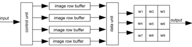
each pixel within a n×n region is delivered in parallel a n×n buffer, as shown in Fig.11, where 242

the "control" unit delivers control data (address and read/write enable) for the BRAM modules, one 243

entire row is stored in each BRAM. Finally the "data" unit delivers n×n pixels in parallel. In our 244

implementation, there is 1 circular buffer of 13×13 pixels/bytes, 1 circular buffer of 17×17 and 2 245

circular buffers of 3×3. For more details see [23]. 246

(a) General formulation of a 3×3 circular buffer

(b) FPGA architecture for the circular buffers

Figure 11.The circular buffers architecture. For a n×n patch, a shift mechanism "control" unit manages the read/write addresses of n+1 BRAMs. In this formulation n BRAMs are in read mode and one BRAM is in write mode in each clock cycle. Then, the n×n buffer delivers logic registers with all pixels within the patch in parallel.

4.2.2. Curl estimation 247

In Fig. 12, the curl architecture is shown. First, one "circular buffer" holds 3 rows of the frame 248

beingprocessedand allows for local parallel access of a 3×3 patch that facilitates parallel processing. 249

Then, image gradients (∂ f (x_∂x,y), ∂ f (x_∂y,y)) are computed. Another "circular buffer" holds 3 rows of the 250

gradient image previously computed and delivers a 3×3 patch for the next step. Second derivatives 251 (∂ ∂y ∂ f (x,y) ∂x , ∂ ∂x ∂ f (x,y)

∂y ) are computed inside the "derivative" unit. Finally, the curl of the input image is 252

computed by the "curl" unit. 253

Figure 12.FPGA architecture for the "curl" unit 4.3. Depth estimation

254

In Fig.13, the depth estimation architecture is shown. Let "pix1 [7;0]", "pix2 [7:0]" be the pixel 255

stream for the optical flow at current frame (Eq.6); first, the "multiplier" unit computes the square value 256

of the input data. Then, the "adder" unit carries out the addition process for both components(∆2_x,∆2y).

257

Finally, the "sqrt" unit computes the depth in the scene, using Eq.9. In order to achieve high efficiency 258

in the square root computation, we adapted the architecture developed by Yamin Li and Wanming 259

Chu [38]. This architecture uses a shift register mechanism and compares the more significant/less 260

significant bits to achieving the root square operation without using embedded multipliers. 261

Figure 13.FPGA architecture for the "depth estimation" unit 5. Result and discussion

262

The developed FPGA architecture was implemented in an FPGA Cyclone IV EP4CGX150CF23C8 263

of Altera. All modules were designed via Quartus II Web Edition version 10.1SP1 and, all modules 264

were validated via post-synthesis simulations performed in ModelSim Altera. For all tests, we consider 265

k=3, s=2 (Eq.4and5) since these values provided a relatively "good" performance forrealworld 266

scenarios. In practice, we recommend these values as reference. Higher k =3, s=2 values could 267

provide higher accuracy, however, processing speed and hardware requirements can be increased. On 268

the other hand, lower k=3, s=2 values should provide higher performance in terms of hardware 269

requirements/processing speed but accuracy could decrease. The full hardware resource consumption 270

of the architecture is shown in Table1. Our algorithm formulation allows for a compact system 271

design; it requires 66% of the total logic elements of the FPGA Cyclone IV EP4CGX150CF23C8. For 272

memory bits, our architecture uses 74% of the total resources, this represents 26 block RAMs consumed 273

mainly in the circular buffers. These hardware utilization enables to target a relatively small FPGA 274

device and therefore could be possible a small FPGA-based smart camera, suitable for real-time 275

embedded applications. In the following subsections comparisons with previous work are presented. 276

For optical flow, comparisons with previous FPGA-based optical flow algorithms are presented.For

277

depth estimation, we presented a detailed discussion about the performance and limitations of the

278

proposed algorithm compared with the current state of the art.

279

5.1. Performance for the optical flow algorithm 280

Table 1.Hardware resource consumption for the developed FPGA architecture. Consumption/image resolution

Resource 640×480 320×240 256×256

Total logic elements 69,879 (59%) 37,059 (31%) 21,659 (18%) Total pins 16 (3%) 16 (3%) 16 (3%) Total Memory Bits 618,392 (15%) 163,122 (4%) 85,607 (2%) Embedded multiplier elements 0 (0%) 0 (0%) 0 (0%)

Total PLLs 1 (25%) 1 (25%) 1 (25%)

In comparison with previous work, in Table2we present hardware resource utilization between 281

our FPGA architecture and previous FPGA-based optical flow algorithms. There are several works 282

[22,25–27] whose FPGA implementations aims to parallelize all recursive operations in the original 283

mathematical formulation. Unfortunately, most popular formulations such as those based in KTL 284

[28] or Horn-Schunck [33], have iterative operations that are hard to parallelize. As result, most 285

previous works have relatively high hardware occupancy/implementations compared with a full 286

parallelizable design approach. Compared with previous works, our FPGA architecture outperform 287

most previous works, for similar image resolution, less logic elements and memory bits than [25,29], 288

and less logic elements and memory bits than [27]. [27] decreases the memory usage by a multiscale 289

coding which makes possible to store only half of the original image, however, this reduction involves 290

pixel interpolation for some cases and this increases the logic elements usage. For [22], the authors 291

introduced an iterative-parallel approach; this makes possible to achieve low hardware requirements 292

but processing speed is low. Finally, for [26], a filtering-based approach makes possible to achieve low 293

hardware requirements with relatively high accuracy and high processing speed but the algorithmic 294

formulation requires to store several entire frames, requiring large external memory (near 250 MB for 295

store 3 entire frames), this increase the system size and cost. 296

Table 2.Hardware resource consumption comparisons

Method Logic elements Memory bits Image resolution Martín et al. [22] (2005) 11,520 147,456 256×256 Díaz et al. [25] (2006) 513,216 685,670 320×240 Wei et al. [26] (2007) 10,288 256 MB (DDR) 640×480 Barranco et al. [27] (2012) 82,526 573,440 640×480 Honegger et al. [29] (2012) 49,655 1,111,000 376×240 Our work* 69,879 624,244 640×480 Our work* 37,059 163,122 320×240 Our work* 21,659 85,607 256×256 *Operating frequency = 50 MHz

In Table3, speed processing for different image resolutions is shown. We synthesized different 297

versions of our FPGA architecture (Fig.8), and we adapted the circular buffers in order to work with 298

all tested image resolutions. Then, we carried out post-synthesis simulation in ModelSim Altera. In 299

all cases, our FPGA architecture reached real-time processing. When compared with previous work 300

(Table4), our algorithm provided the highest speed processing, it outperforms several previous work 301

[22,25–27,29], and for HD images, our algorithm reaches real-time processing: more than 60 fps for 302

1280×1024 image resolution. 303

Table 3.Processing speed for different image resolutions Resolution Frames/s Pixels/s 1280×1024 68 90,129,200

640×480 297 91,238,400 320×240 1,209 92,880,000 256×256 1,417 92,876,430 *Operating frequency = 50 MHz

Table 4.Processing speed comparisons

Method Resolution Frames/s Pixels/s Martín et al. [22] 256×256 60 3,932,160 Díaz et al. [25] 320×240 30 2,304,000 Wei et al. [26] 640×480 64 19,550,800 Barranco et al. [27] 640×480 31 9,523,200 Honegger et al. [29] 376×240 127 11,460,480 Our work 640×480 297 91,238,400

In Fig.14, qualitative results for this work compared with previous work are shown. In a first

304

experimentwe used the ”Garden” dataset since previous work [22,25,26] used this dataset as reference. 305

When compared with previous work (Fig. 14), our algorithm provides high performance under 306

real world scenarios, it outperforms several previous work [22,25,26], quantitatively closer to the 307

ground truth (error near to 9%) compared with other FPGA-based approaches.In a second experiment

308

quantitative and qualitative results for the KITTI dataset [39], are shown. In all cases our algorithm 309

provides high performance, it reaches an error near to 10% with several test sequences, as shown in 310

Fig.15.In both experiments we compute the error by comparing the ground truthΩx(x, y),Ωy(x, y)

311

(provided with the dataset) with the computed optical flow∆x(x, y),∆y(x, y). First, we compute the

312

local error (the error magnitude at each point of the input image) as defined in Eq.10; where i, j is the

313

input image resolution. Then, a global error(Ξ)can be computed as shown in Eq.11; where i, j is the

314

input image resolution. ξ(x, y)is the local error at each pixel in the reference image and the global

315

error(Ξ)is the percentage of pixels in the reference image in which local error is higher to zero.

316 ξ(x, y) = x=i

∑

∑

∑

∑

(a) input image (b) ground truth (c) Martín et al. [22]

(d) Wei et al. [26] (e) Díaz et al. [25] (f) this work (error = 9%) Figure 14.Accuracy performance for different FPGA-based optical flow algorithms.

(a) input image (b) ground truth (c) flow estimation (error = 11%)

(a) input image (b) ground truth (c) flow estimation (error = 12%)

(a) input image (b) ground truth (c) flow estimation (error = 11%)

(a) input image (b) ground truth (c) flow estimation (error = 12%) Figure 15.Optical flow: quantitative/qualitative results for the KITTI dataset

5.2. Performance for the depth estimation step 318

In Fig.15, quantitative and qualitative results for the KITTI dataset [39], are shown. In all cases 319

our algorithm provides rough depth maps compared with stereo-based or deep learning approaches 320

[40,41] but with real-time processing and with the capability to be implemented in embedded hardware, 321

suitable for smart cameras.To our knowledge, previous FPGA-based approaches are limited; there are

322

several GPU-based approaches but in these cases most of the effort was for accuracy improvements and

323

real-time processing or embedded capabilities were not considered so, in several cases, details about

324

the hardware requirements or the processing speed are not provided [42–44]. In Table5quantitative

325

comparisons between our algorithm and the current state of the art are presented. For previous

326

works, the RMS error, hardware specifications and processing speed were obtained from the published

327

manuscripts while for our algorithm we computed the RMS error as indicated by the KITTI dataset,

328

[45]. For accuracy comparisons, most previous works [42–44,46–48] outperform our algorithm (near

329

15% more accurate than ours); however, our algorithm outperform all of them in terms of processing

330

speed (a processing speed up to 128 times faster than previous works) and with embedded capabilities

331

(making it possible to develop a smart camera/sensor suitable for embedded applications).

332

Table 5.Depth estimation process in the literature: performance and limitations for the KITTI dataset.

Method Error (RMS) Speed Image resolution Approach

Zhou et al. [42](2017) 6.8% - 128×416 DfM-based* -Yang et al. [46](2017) 6.5% 5 fps 128×416 CNN-based* GTX 1080 (GPU) Mahjourian et al. [47](2018) 6.2% 100 fps 128×416 DfM-based* Titan X (GPU)

Yang et al. [43](2018) 6.2% - 830×254 DfM-based* Titan X (GPU) Godard et al. [44](2018) 5.6% - 192×640 CNN-based*

-Zou et al. [48](2018) 5.6% 1.25 fps 576×160 DfM-based* Tesla K80 (GPU) Our work 21.5% 192 fps 1241×376 DfM-based Cyclone IV (FPGA) *DfM: Depth from Motion, CNN: Convolutional Neural Network

(a) input image (b) ground truth (c) depth estimation (error = 21%)

(a) input image (b) ground truth (c) depth estimation (error = 22%)

(a) input image (b) ground truth (c) depth estimation (error = 21%)

(a) input image (b) ground truth (c) depth estimation (error = 22%) Figure 16.Depth estimation: quantitative/qualitative results for the KITTI dataset

Finally, in Fig.17an example of 3D reconstruction using our approach is shown. Our depth maps 333

allowfor a real-time dense 3D reconstruction. Previous works like the ORB-SLAM [49] or LSD-SLAM 334

[50] compute motion and depth in 2 to 7% of all image pixels, while ours compute 80% of the image 335

pixels. Then, our algorithm improves by around 15 times the current state of the art, making possible 336

real-time dense 3D reconstructions and with the capability to be implemented inside FPGA devices, 337

suitable for smart cameras. 338

339

(a) Input image

(b) Depth map

(c) 3D reconstruction

Figure 17.The KITTI dataset: Sequence 00; 3D reconstruction by the proposed approach. Our algorithm provides rough depth maps (lower accuracy compared with previous algorithms) but with real-time processing and with the capability to be implemented in embedded hardware; as result, real-time dense 3D reconstructions can be obtained and, these can be exploited by several real world applications such as, augmented reality, robot vision and surveillance, autonomous flying, etc.

6. Conclusions 340

Depth from Motion is the problem of depth estimation using information from a single moving

341

camera. Although several Depth from Motion algorithms were developed, previous works have low

342

processing speed and high hardware requirements that limits the embedded capabilities. In order to

343

solve these limitations in this work we have proposed a new depth estimation algorithm whose FPGA

344

implementation deliver high efficiency in terms of algorithmic parallelization. Unlike previous works,

345

depth information is estimated in real time inside a compact FPGA device, making our mathematical

346

formulation suitable for smart embedded applications.

347

Comparted with the current state of the art, previous algorithms outperform our algorithm in

348

terms of accuracy but our algorithm outperforms all previous approaches in terms of processing speed

349

and hardware requirements; these characteristics makes our approach a promising solutions for the

350

current embedded systems. We believed that several real world applications such as augmented reality,

351

robot vision and surveillance, autonomous flying, etc., can take advantages by applying our algorithm

352

since it delivers real-time depth maps that can be exploited to create dense 3D reconstructions or other

353

abstractions useful for the scene understanding.

354

Author Contributions:Conceptualization, Abiel Aguilar-González, Miguel Arias-Estrada and François Berry. 355

Investigation, Validation and Writing—Original Draft Preparation: Abiel Aguilar-González. Supervision and 356

Writing—Review & Editing: Miguel Arias-Estrada and François Berry. 357

Funding:This research received no external funding. 358

Acknowledgments:This work has been sponsored by the French government research program "Investissements 359

d’avenir" through the IMobS3 Laboratory of Excellence (ANR-10-LABX-16-01), by the European Union through the 360

program Regional competitiveness and employment, and by the Auvergne region. This work has been sponsored 361

by Campus France through the scholarship program "bourses d’excellence EIFFEL", dossier No. MX17-00063 and 362

by the National Council for Science and Technology (CONACyT), Mexico, through the scholarship No. 567804.. 363

Conflicts of Interest:The authors declare no conflict of interest. 364

365

1. Hengstler, S.; Prashanth, D.; Fong, S.; Aghajan, H. MeshEye: a hybrid-resolution smart camera mote for 366

applications in distributed intelligent surveillance. Proceedings of the 6th international conference on 367

Information processing in sensor networks. ACM, 2007, pp. 360–369. 368

2. Aguilar-González, A.; Arias-Estrada, M. Towards a smart camera for monocular SLAM. Proceedings of 369

the 10th International Conference on Distributed Smart Camera. ACM, 2016, pp. 128–135. 370

3. Carey, S.J.; Barr, D.R.; Dudek, P. Low power high-performance smart camera system based on SCAMP 371

vision sensor. Journal of Systems Architecture 2013, 59, 889–899. 372

4. Birem, M.; Berry, F. DreamCam: A modular FPGA-based smart camera architecture. Journal of Systems 373

Architecture 2014, 60, 519–527. 374

5. Bourrasset, C.; Maggianiy, L.; Sérot, J.; Berry, F.; Pagano, P. Distributed FPGA-based smart camera 375

architecture for computer vision applications. Distributed Smart Cameras (ICDSC), 2013 Seventh 376

International Conference on. IEEE, 2013, pp. 1–2. 377

6. Bravo, I.; Baliñas, J.; Gardel, A.; Lázaro, J.L.; Espinosa, F.; García, J. Efficient smart cmos camera based on 378

fpgas oriented to embedded image processing. Sensors 2011, 11, 2282–2303. 379

7. Köhler, T.; Röchter, F.; Lindemann, J.P.; Möller, R. Bio-inspired motion detection in an FPGA-based smart 380

camera module. Bioinspiration & biomimetics 2009, 4, 015008. 381

8. Olson, T.; Brill, F. Moving object detection and event recognition algorithms for smart cameras. Proc. 382

DARPA Image Understanding Workshop, 1997, Vol. 20, pp. 205–208. 383

9. Norouznezhad, E.; Bigdeli, A.; Postula, A.; Lovell, B.C. Object tracking on FPGA-based smart cameras 384

using local oriented energy and phase features. Proceedings of the Fourth ACM/IEEE International 385

Conference on Distributed Smart Cameras. ACM, 2010, pp. 33–40. 386

10. Fularz, M.; Kraft, M.; Schmidt, A.; Kasi ´nski, A. The architecture of an embedded smart camera for intelligent 387

inspection and surveillance. In Progress in Automation, Robotics and Measuring Techniques; Springer, 2015; pp. 388

43–52. 389

11. Haritaoglu, I.; Harwood, D.; Davis, L.S. W 4: Real-time surveillance of people and their activities. IEEE 390

Transactions on pattern analysis and machine intelligence 2000, 22, 809–830. 391

12. Biswas, J.; Veloso, M. Depth camera based indoor mobile robot localization and navigation. Robotics and 392

Automation (ICRA), 2012 IEEE International Conference on. IEEE, 2012, pp. 1697–1702. 393

13. Stowers, J.; Hayes, M.; Bainbridge-Smith, A. Altitude control of a quadrotor helicopter using depth map 394

from Microsoft Kinect sensor. Mechatronics (ICM), 2011 IEEE International Conference on. IEEE, 2011, pp. 395

358–362. 396

14. Scharstein, D.; Szeliski, R. A taxonomy and evaluation of dense two-frame stereo correspondence 397

algorithms. International journal of computer vision 2002, 47, 7–42. 398

15. Subbarao, M.; Surya, G. Depth from defocus: a spatial domain approach. International Journal of Computer 399

Vision 1994, 13, 271–294. 400

16. Chen, Y.; Alain, M.; Smolic, A. Fast and accurate optical flow based depth map estimation from light fields. 401

Irish Machine Vision and Image Processing Conference (IMVIP), 2017. 402

17. Zhang, J.; Singh, S. Visual-lidar odometry and mapping: Low-drift, robust, and fast. Robotics and 403

Automation (ICRA), 2015 IEEE International Conference on. IEEE, 2015, pp. 2174–2181. 404

18. Schubert, S.; Neubert, P.; Protzel, P. Towards camera based navigation in 3d maps by synthesizing depth 405

images. Conference Towards Autonomous Robotic Systems. Springer, 2017, pp. 601–616. 406

19. Maddern, W.; Newman, P. Real-time probabilistic fusion of sparse 3d lidar and dense stereo. Intelligent 407

Robots and Systems (IROS), 2016 IEEE/RSJ International Conference on. IEEE, 2016, pp. 2181–2188. 408

20. Dai, A.; Chang, A.X.; Savva, M.; Halber, M.; Funkhouser, T.A.; Nießner, M. ScanNet: Richly-Annotated 3D 409

Reconstructions of Indoor Scenes. 2017. 2, 10. 410

21. Liu, H.; Li, C.; Chen, G.; Zhang, G.; Kaess, M.; Bao, H. Robust Keyframe-based Dense SLAM with an 411

RGB-D Camera. arXiv preprint arXiv:1711.05166 2017. 412

22. Martín, J.L.; Zuloaga, A.; Cuadrado, C.; Lázaro, J.; Bidarte, U. Hardware implementation of optical flow 413

constraint equation using FPGAs. Computer Vision and Image Understanding 2005, 98, 462–490. 414

23. Aguilar-González, A.; Arias-Estrada, M.; Pérez-Patricio, M.; Camas-Anzueto, J. An FPGA 2D-convolution 415

unit based on the CAPH language. Journal of Real-Time Image Processing 2015, pp. 1–15. 416

24. Pérez-Patricio, M.; Aguilar-González, A.; Arias-Estrada, M.; Hernandez-de Leon, H.R.; Camas-Anzueto, 417

J.L.; de Jesús Osuna-Coutiño, J. An fpga stereo matching unit based on fuzzy logic. Microprocessors and 418

Microsystems 2016, 42, 87–99. 419

25. Díaz, J.; Ros, E.; Pelayo, F.; Ortigosa, E.M.; Mota, S. FPGA-based real-time optical-flow system. IEEE 420

transactions on circuits and systems for video technology 2006, 16, 274–279. 421

26. Wei, Z.; Lee, D.J.; Nelson, B.E. FPGA-based Real-time Optical Flow Algorithm Design and Implementation. 422

Journal of Multimedia 2007, 2. 423

27. Barranco, F.; Tomasi, M.; Diaz, J.; Vanegas, M.; Ros, E. Parallel architecture for hierarchical optical 424

flow estimation based on FPGA. IEEE Transactions on Very Large Scale Integration (VLSI) Systems 2012, 425

20, 1058–1067. 426

28. Tomasi, C.; Kanade, T. Detection and tracking of point features. School of Computer Science, Carnegie Mellon 427

Univ. Pittsburgh 1991. 428

29. Honegger, D.; Greisen, P.; Meier, L.; Tanskanen, P.; Pollefeys, M. Real-time velocity estimation based on 429

optical flow and disparity matching. IROS, 2012, pp. 5177–5182. 430

30. Chao, H.; Gu, Y.; Napolitano, M. A survey of optical flow techniques for robotics navigation applications. 431

Journal of Intelligent & Robotic Systems 2014, 73, 361–372. 432

31. Dosovitskiy, A.; Fischer, P.; Ilg, E.; Hausser, P.; Hazirbas, C.; Golkov, V.; Van Der Smagt, P.; Cremers, D.; 433

Brox, T. Flownet: Learning optical flow with convolutional networks. Proceedings of the IEEE International 434

Conference on Computer Vision, 2015, pp. 2758–2766. 435

32. Ilg, E.; Mayer, N.; Saikia, T.; Keuper, M.; Dosovitskiy, A.; Brox, T. Flownet 2.0: Evolution of optical flow 436

estimation with deep networks. IEEE conference on computer vision and pattern recognition (CVPR), 437

2017, Vol. 2, p. 6. 438

33. Horn, B.K.; Schunck, B.G. Determining optical flow. Artificial intelligence 1981, 17, 185–203. 439

34. Khaleghi, B.; Shahabi, S.M.A.; Bidabadi, A. Performace evaluation of similarity metrics for stereo 440

corresponce problem. Electrical and Computer Engineering, 2007. CCECE 2007. Canadian Conference on. 441

IEEE, 2007, pp. 1476–1478. 442

35. Geiger, A.; Lenz, P.; Stiller, C.; Urtasun, R. Vision meets robotics: The KITTI dataset. The International 443

Journal of Robotics Research 2013, 32, 1231–1237. 444

36. Baker, S.; Scharstein, D.; Lewis, J.; Roth, S.; Black, M.J.; Szeliski, R. A database and evaluation methodology 445

for optical flow. International Journal of Computer Vision 2011, 92, 1–31. 446

37. Fortun, D.; Bouthemy, P.; Kervrann, C. Optical flow modeling and computation: a survey. Computer Vision 447

and Image Understanding 2015, 134, 1–21. 448

38. Li, Y.; Chu, W. A new non-restoring square root algorithm and its VLSI implementations. Computer Design: 449

VLSI in Computers and Processors, 1996. ICCD’96. Proceedings., 1996 IEEE International Conference on. 450

IEEE, 1996, pp. 538–544. 451

39. Geiger, A.; Lenz, P.; Stiller, C.; Urtasun, R. Vision meets robotics: The KITTI dataset. The International 452

Journal of Robotics Research 2013, 32, 1231–1237. 453

40. Fu, H.; Gong, M.; Wang, C.; Batmanghelich, K.; Tao, D. Deep Ordinal Regression Network for Monocular 454

Depth Estimation. IEEE Conference on Computer Vision and Pattern Recognition (CVPR); , 2018. 455

41. Bo Li, Yuchao Dai, M.H. Monocular Depth Estimation with Hierarchical Fusion of Dilated CNNs and 456

Soft-Weighted-Sum Inference 2018. 457

42. Zhou, T.; Brown, M.; Snavely, N.; Lowe, D.G. Unsupervised learning of depth and ego-motion from video. 458

CVPR, 2017, Vol. 2, p. 7. 459

43. Yang, Z.; Wang, P.; Wang, Y.; Xu, W.; Nevatia, R. LEGO: Learning Edge with Geometry all at Once by 460

Watching Videos. Proceedings of the IEEE Conference on Computer Vision and Pattern Recognition, 2018, 461

pp. 225–234. 462

44. Godard, C.; Mac Aodha, O.; Brostow, G. Digging Into Self-Supervised Monocular Depth Estimation. arXiv 463

preprint arXiv:1806.01260 2018. 464

45. Uhrig, J.; Schneider, N.; Schneider, L.; Franke, U.; Brox, T.; Geiger, A. Depth Prediction 465

Evaluation. http://www.cvlibs.net/datasets/kitti/eval_odometry_detail.php?&result=

466

fee1ecc5afe08bc002f093b48e9ba98a295a79ed, 2017. 467

46. Yang, Z.; Wang, P.; Xu, W.; Zhao, L.; Nevatia, R. Unsupervised Learning of Geometry with Edge-aware 468

Depth-Normal Consistency. arXiv preprint arXiv:1711.03665 2017. 469

47. Mahjourian, R.; Wicke, M.; Angelova, A. Unsupervised Learning of Depth and Ego-Motion from Monocular 470

Video Using 3D Geometric Constraints. Proceedings of the IEEE Conference on Computer Vision and 471

Pattern Recognition, 2018, pp. 5667–5675. 472

48. Zou, Y.; Luo, Z.; Huang, J.B. Df-net: Unsupervised joint learning of depth and flow using cross-task 473

consistency. European Conference on Computer Vision. Springer, 2018, pp. 38–55. 474

49. Mur-Artal, R.; Montiel, J.M.M.; Tardos, J.D. ORB-SLAM: a versatile and accurate monocular SLAM system. 475

IEEE Transactions on Robotics 2015, 31, 1147–1163. 476

50. Engel, J.; Schöps, T.; Cremers, D. LSD-SLAM: Large-scale direct monocular SLAM. European Conference 477

on Computer Vision. Springer, 2014, pp. 834–849. 478

Sample Availability:Samples of the compounds ... are available from the authors. 479

c

2018 by the authors. Submitted to Sensors for possible open access publication under the terms and conditions 480

of the Creative Commons Attribution (CC BY) license (http://creativecommons.org/licenses/by/4.0/). 481