Design and evaluation of multimicroprocessor systems

DESIGN AND EVALUATION OF

MULTIMICROPROCESSOR SYSTEMS

by

AMAR GUPTA

B. Tech., I.I.T., Kanpur, India

(1974)

SUBMITTED IN

P.ARTIAL FULFILLMENT

OF THE REQUIREMENTS FOR THE

DEGREE OF

MASTER OF SCIENCE IN

MANAGEMENT

at the

MASSACHUSETTS INSTITUTE OF TECHNOLOGY

O

Sloani School -f Management

May 1, 1980 Certified b Accepted by y / "Hoo-min D. Toong / Thesis Supervisor

SMichael

_{S. Scott Morton}

DESIGN AND EVALUAT1OC OF MULTLMICROPRO CESSOR SYSTEMS

by AMAR GUPTA

Submitted to the Alfred P. Sloan School of Management on May 1, 1980 in partial fulfillment of the requirements for the Degree of Master of Science

ABSTRACT

The next few years will witness widespread application of multi-microprocessor systems for diverse purposes. The operation of

such systems is presently constrained by bus contention problems, and by increased complexity of the control program software. An interactive

package is developed for analytic modeling of multimicroprocessor

systems. This package adapts readily to arbitrary system configurations employing a central time-shared bus, and serves as a useful tool in the design and performance evaluation of multimicroprocessor systems.

In this thesis, the interactive package is used to evaluate four bus architectures in different job environments. The results have been cross-validated using a simulation model.

Thesis Supervisor: Hoo-min D. Toong

ACKNOWLEDGEM1ENTS

This thesis could not have been written without the encouragement, support, and insightful suggestions of my supervisor, Professor Hoo-min D. Toong; he has been a teacher, guide and friend, all in one.

I am grateful to all the members of the project team; they

provided a valuable forum for all my brainstorming ideas. In particular, I would like to thank Svein 0. Strommen for his relevant comments and criticisms, Tarek Abdel-Hamid for the simulation models, and

Benjamin Chou for his support in the later phases.

AMAR GUPTA May 1, 1980

TABLE OF CONTENTS

Chapter Heading Page

1 INTRODUCTION ... 5

2 I pPS ... 12

3 APPLICATIONS AND THEORETICAL CONSTRAINTS ... 36

4 RESPONSE TIMINGS ... ... 52

5 VALIDATION OF IMPS ... 65

6 CONCLUSION ... 74

CHAPTER ONE

INTRODUCTION

1.1 BACKGROUND

As computer system complexity grows, so do total costs. Tech-nological innovations are rapidly decreasing hardware costs, but these decreases are more than offset by investments needed to develop and/ or rewrite software. Each new technology (e.g. microprocessors) results in a software "reinvention of the wheel." As this complexity increases, the labor intensive software reinvention costs escalate. For example, office computers of today have limited word processing capabilities. In order to permit graphic outputs, remote communica-tions, audio input and output facilities and similar features that are. desirable for the office computer of tomorrow, the present systems architectures will most probably have to be redesigned, and control program software developed for each new function. It is estimated that with the current 30% increase in microprocessor designs per annum, and a 100% implementation effort increase for design, the total

implementation costs will exceed $1.25 million in 1985, and more than 1,000,000 software engineers will be needed for all such applications by 1990 (34, 35).

In order to curb these escalating costs, a long term stable applications base is needed in this area. One way is to develop new

with the same basic structure; the system must be modular and easy to use, and hardware changes should be transparent to the user. (This

is vital since the technology is changing so rapidly). Multiprocessors, if designed properly allow this modulanty, long term growth, ease of use, and possibly, as a side benefit, large computation capability.

One commonly identifies three basic motivations for the development of multiprocessors (1). These are as follows:

a) THROUGHPUT. Multiple processors permit increased throughput by simultaneous, rather than simply concurrent, processing of parallel tasks;

b) FLEXIBILITY. Multiple-processor systems differ from

former provide some level of close-sharing of recources,

e.g. shared memory, input/output devices, software libraries, not allowed by separate computer systems. Jobs, too "large" to run on a single processor, can be executed on the multiprocessor system. Flexibility also permits smooth system growth through incremental expansion by adding new processor modules;

c) RELIABILITY. Multiprocessor systems possess the potential for detecting and correction/elimination of defective processing modules. This leads to high availability,

a key characteristic to fault tolerant systems and a fail-soft capability. Traditional fault-tolerant systems attempt to achieve both high availability and high integrity by using duplexed and triplexed functional units. (2)

The last five years have witnessed a spurt in activities relating to research and development of multimicroprocessor systems. The

overwhelming factor has been the rapidly plummeting cost of semi-conductor hardware (e.g. microprocessors) accompanied by an enormous increase in their computing power and capabilities. The availability of microprogrammable microprocessors has been an added boon and

permits easier adaptation of microprocessors to multiprocessor systems.

1.2 PROBLEM AREAS

The following problem areas exist for uniprocessor systems:

1) The memory address space is too small and there is a lack of memory management and memory protection features.

2) Assembly language programming is difficult and extremely time-consuming for anything but the shortest program. This problem can be alleviated though, by the use of a high-level language.

3) The memory usage is extremely high and inefficient.

4) There is no capability to execute an indivisible TEST and SET instruction. This facility will be necessary for resource allocation in a multiprocessor environ-ment.

5) The 8-bit wood size of the microprocessor in most common usage is just too small for extended precision

operations.

6) There is no ability to configure an operating system with priveleged states or priveleged instructions.

An operating system would include at least a problem state and a supervisor state. (3)

Today, 16 bit word size microprocessors are available; however, several of the above problems continue to be areas of sustained research activities.

As compared to uniprocessor configurations, multiprocessor systems are characterised by increased complexity in two major areas:

a) Interconnection mechanism.

In a system with 'N' processors, if each processor is to directly co-mmunicate _{with every other (N-1)}

processor, then N.(N-1) connections would be required. As the value of N increases, the number of intercon-nections increases as a square of N, and this makes the strategy costly to implement. The problem is identical to telephone systems wherein it was realized very early that line sharing is necessary in order to reduce

costs. In the multimicroprocessor environment, such sharing has been attempted in the form of parallel buses, ring buses, cross point switches, trunk systems, and multiple buses. Haagens (5) has summarised these characteristics of these designs, and has attempted a unique split transaction Time-Shared Bus that permits a single bus to be optimized for catering to very high communication loads.

In essence, the interconnection mechanism represents the hardware facet of the problem.

b) Operating System

For optimal utilization of the processing elements, the "distributed operating system" (DOS) is now required to perform additional coordination, scheduling and

dispatching functions. Further, DOS must select "the means by which computing tasks are to be divided among the processors so that for the duration of that

.10

unit of work, each processor has logically consistent instructions and data." (6)

This must be done without replicating the program routines, and without compromising the "privacy" of the program at any stage. Finally the design must implicitely provide for graceful degradation in case any element fails. Thus each processing element should be capable of undertaking the "distributed operating system" functions. This resilience is especially critical where the system application dictates a maximum system throughout.

1.3 PRESENT WORK

The Center for Information Systems Research is involved in the design, development and implementation of a multi-microprocessor system which is hoped to be the blueprint of systems architectures for the previously outlined needs during the 1985-1995 timeframe. This system features much tighter processor coupling, higher

resilience and much higher throughput than the systems under develop-ment at Carnegie-Mellon (7) and Stanford (8).

The work on this multimicroprocessor project can be divided into the following phases:

(i) Analysis of microprocessors, and their suitability as basic elements in larger systems;

(ii) Evaluation of existing interconnection protocols in order to identify the optimal bus architecture;

(iii) Development of a distributed operating system;

(iv) Final implementation.

Obviously, the above phases have considerable overlap in terms of time. Phase (i) is completed and the effort is documented in (11, 12, 13, 14, 15).

The author has been heavily involved in phase (ii). In this search for an optimum bus architecture, it was considered desirable to develop a computer-based decision support system (9, 10) to

facilitate the design and evaluation process, both for interconnection mechanisms as well as for the distributed operating system. In

the next chapter, this design aid is described in detail. The following chapters examplify the use of this facility to analyze various bus

CHAPTER

2.1 INTRODUCTION

In the previous chapter, we saw that with the availability of low cost microprocessors, there is a growing trend towards multi-micropro-cessor systems. Presently, research is focussed on the evolution of improved inter-processor communication facilities. Whereas the constraint in single processor systems is the speed of the processor itself, the constraint in multi-processor systems is the speed of the

bus used for communicating between processors. As the number of processors increases, so does the probability of simultaneous request for bus

service by more than one processor. This bus contention problem has been examined among others by (5,24).

This chapter describes a tool, entitled IMfPS (acronym for Inter-active Multi-Microprocessor Performance System), developed to study single time-shared bus based multimicroprocessor systems. DLMTS, developed at the Center for Information System Research (CISR) of MIT, is an example of the use of queueing theory for the development of analytic models of computer systems. In this chapter, the model is developed, and the broad features of IMMPS outlined. Finally, the effect of a new message protocol on the system throughput are analyzed

2.2 Multi-microprocessor systems

A single processor system can be represented as shown in Figure 2.1.

Figure 2.1 Single Processor System

When several of such mono-processor systems are connected together,

I

any element of the system (CPU, Memory or /0) _{must be capable of}

communi-cating with any other element of that system (CPU, Memory or /0), and a typical two-processor system is shown in Figure 2.2.

I

_J

_I

It is obvious that as the number of processors increases, the load on the inter-face increases sharply. For the mono-processor configuration shown in Fig. 2.1, the number of possible message paths is 3!/2! = 3; for the configuration in Figure 2.2, the number of paths = 6! = 15. Several authors have proposed

21 41

multi-bus systems (Ref. 5 contains a good summary), but the cost of such

multiple-bus interconnections increases as a square of the number of processors. On the other hand, if only one bus is used, the contention problem between

different messages may become critical.

In order to reduce the load on the bus, it is now becoming common for individual processors to have cache memories. On the other side, the

intelli-gence of memory and I/0 units is increasing, and as such the dividing line

cate-gorised into two major groups:

(a) Primary Processing Modules (PPM):

These are elements with higher level of intelligence; these elements control the operation of other elements. A traditional CPU is an example

of a PPM: another term for such modules is "Masters";

(b) Tertiary Processing Modules (TPM):

These are elements with lower or zero level of intelligence; typical examples are memory, /0 processors. The operation of TPM is initiated

In traditional single processor systems, there is one and only one PPM, and typically more than one TPM. In multi-microprocessor systems, there are several PPMs, each "controlling" the functions of a number of other TrM's,

in coordination with other PPMs. The term PM or Processing Module is used

to represent an element which may be either a PPM or a TPM.

The term "message" is used in the literature to represent a wide

spectrum of communication levels. In this thesis messages are considered

to be of one of the following two main types:

(a) "m-message"(short for macro-message). This type of message is initiated

by any PPM, and includes all the resulting supplementary processes and communications that are directly attributable to the PPM's command. In general, an m-message will involve one or more PPMs, several TPMs and a

sequence of bus usages disjoint over time.

(b) "e-message" (short for elementary-message). Such messages require a single

usage of bus, and involve only two PMs (both PPMs or both TPMs or one PPM

and one TPM). An example of e-message is a simple "WRITE" from a processor to a memory. Essentially, an e-message denotes the most elementary message communication between two processing modules.

In general, each m-message will result in one or more e-messages. A simple store of type Register to Memory (direct addressing) will usually result in

a single WRITE message that includes the value to be written. _{This is an} example of an m-message resulting in a single e-message. On the other hand, a READ-MODIFY-WRITE sequence may be a single m-message, but would necessarily involve a sequence of e-messages.

2. 3. PARAMETERS FOR THE MODEL

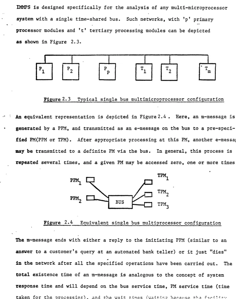
IMMPS is designed specifically for the analysis of any multi-microprocessor system with a single time-shared bus. Such networks, with 'p' primary processor modules and 't' tertiary processing modules can be depicted

as shown in Figure 2.3.

Figure 2.3 Typical single bus multimicroprocessor configuration

- : An equivalent representation is depicted in Figure2.4 . Here, an m-message is * generated by a PPM, and transmitted as an e-message on the bus to a

pre-speci-fied PM(PPM or TPM). After appropriate processing at this PM, another e-message may be transmitted to a definite PM via the bus. In general, this process is repeated several times, and a given PM may be accessed zero, one or more times.

TPN

PPM

PP42

TPM2 TPM3

Figure 2.4 Equivalent single bus multiprocessor configuration

The m-message ends with either a reply to the initiating PPM (similar to an answer to a customer's query at an automated bank teller) or it just "dies" in the network after all the specified operations have been carried out. The

total existence time of an m-message is analogous to the concept of system response time and will depend on the bus service time, PM service time (time

taken for the processint), and the wait •times (waitin because -th. f2cli:

Messages:

- number of message types (either as e-messages or m-messages or any appropriate combination provided a given physical message is not repeated)

- the frequency (arrival rate) and priority of each message type. System configuration:

- the system configuration in terms of numbers of different PPMs and TPMs. Details of similar PMs (e.g. memory units with same access time) have to be

specified only once

- the bus time (also called service time) required to transmit a message (may

be different for different messages);

-

average processing time for each PM.

In case, the system has been specified in terms of m-messages, the movement path

of each type of message (number of requests to each PM) must be specified. For

example, a credit query request may result in two accesses to a particular PPM

and four accesses to a particular TPM.

2.4.

QUEUEING

N'P.TWOK

1MODEL

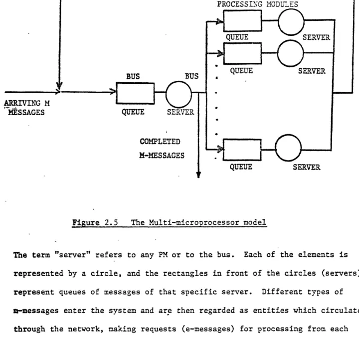
The configurations indicated in Figures 2.3 and 2.4 earlier can be represen-ted by the central server model depicrepresen-ted in Figure 2.5. This is a system with a single bus and multiple processing elements.

PROCESSING MODULES

BUS BUS

ARRIVING M

MESSAGES QUEUE SERVER

COMPLETED M-MESSAGES

QUEUE

SERVER

Figure 2.5 The Multi-microprocessor model

The term "server" refers to any PM or to the bus. Each of the elements is represented by a circle, and the rectangles in front of the circles (servers) represent queues of messages of that specific server. Different types of m-messages enter the system and are then regarded as entities which circulate through the network, making requests (e-messages) for processing from each server they encounter and waiting in queues at times when they make a request

1

,,

I

m

to a busy server. Different messages may be assigned different priorities, or several messages may share the same priority. This affects their chances of getting the bus. A "m-message" may cause several "e-message" involving various processing modules.

The following variables and indices are used:

Index i denotes a specific processing module (1 < i < n) Index j denotes a specific message (m or e type) (1 < J < m) Index k denotes a specific priority (1 < k < 1)

q _{denotes a priority level (1l q < )} n number of PM in the system configuration m number of message types

t

ai gross arrival rate of messages to element i

a gross arrival rate of type j messages in system ak arrival rate of messages with priority k

s_i service time of module i

s _{gross bus service time for message j}

sj' _{bus service time per e-message from message j of priority k} Sk average bus service time per e-message of priority k

NRiJ number of e-messages due to m-message

_j*

Qi queue length of device i

Squeue length of priority k at the bus R_i response time of element i

RDj total device response time for m-message j

R

Ui

Uk

Usk

total system response time for m-message j

average bus response time for m-message k utilization of element i

bus utilization by messages of priority k

weighted bus utilization by messages of priority k

2.4.1 Formulae for bus evaluation

Assuming exponential distribution of interarrival times of messages, exponential distribution of service times required per message, and a single central server (summarized as M/IM/ model), the following formulae are-valid:

ak = Za

sk = (Za..s')/(Za.)

I

U

k

= ak.sk

Rk - k + E Usk/(1-Z ak.Sk)

1--

E a .s

Qk

=

Rk.ak

sum up only those aj, ajsj'

2.4.2 Formulae for device/element evaluation.

For a M/M/I model, and a first come-first serve (FCFS) discipline, regardless of message type and priority, the formulae, for the respective expected values, are as under:

Ui = a .s i

Q

U / (1-Ui)

R

±

_sl

_/(1-U

_{i )}

2.4.3 Formulae for evaluation of individual messages:

The response time for a specific message is composed of two parts:

the total PM response time for that message and the bus response time for that message. The formulae for these components and the total response time are shown below:

n

where s

n8

+

I

NR

Nij

F

Dj

R+

RBUSj

Finally,

R

2.5. _{SALIENT FEATURES OF DLP2S MODEL}

The Interactive Multi-Microprocessor Performance System (DI~PS) is a modified and expanded version of the central server queueing model developed by (25,26). Salient features of the new model will now be discussed:

2. 5.1 Queueing Network Model:

OMPS is a queueing network model based on a Poisson distribution of message generation. The Poisson assumption is close to reality, and gives accurate results (27). It is the only continuous distribu-tion with the "memory-less" property, and further it leads to

relatively simple mathematical formulae. The arrival rate is assumed to be constant and homogenous, and these assumptions have generally given results within 10% of observed results. (28)

2. 5.2 Interactive operation:

The program is written in FORTRAN and operates in an interactive mode. System commands and data parameters can be input in the interactive mode, filed for later use in the file mode, and readily modified in the edit mode. User is prompted to respond by easy to understand questions.

2. 5.3 System configuration:

Presently, DM~PS is set up to accept a maximum of 100 processing modules. This limit can be easily increased, when larger

configura-tions are analysed.

2. 5.4 NACK and TIMEOUT imnlementation:

In the latest implementation of the model, the NACK (short for

for receiving PM or when receiving PM is busy) and TIMEOUT (no reply

signal received in pre-specified time duration) are also imple-mented. Values for these parameters can be inserted and varied by the user.

2.5.5 Average Response Time:

The model outputs average response times for the bus and individual processing elements, plus the average (expected value) queue lengths at various devices. The computed results are arranged by message

type and also by PM type. For initial design, the use of average response time as a ballpark figure is sufficient. Later, when

various system parameters are known more accurately, actual individual figures help in a better comprehension of the entire system.

2.5.6 Sensitivity analysis and graphical outputs:

After obtaining results for a specific configuration, various

parameters (e.g. bus speed, NACK rate, TIMEOUT rate) can be modified and a new output obtained. An easier alternative is to use the option of sensitivity analysis and graphical output. The user can specify the independent variable, the step size (as a percentage of

initial value), the number of iterations or graphical points (maximum of 99), and the range for the average response time which is the dependent variable. The latter, and the type of graph points, can either be specified by -the user or pre-programmed default values

are assumed.

2.5.7 Elaborate warning and error detection routines;

All user specified values are checked, to the extent possible, for correctness and compatibility with other values. User is prompted

in case of errors/potential errors, and amendments are easily done in EDIT mode.

2.5.8 Infinite queues:

An assumption is made that there is no upper limit on the queue lengths at input/output of different PY-s. This is done because finite/queue capacity problems can be mathematically sol-ed only for some cases. A companion simulation model has been used at MIT for finite queue capacity system analysis, and these results

have been very close to the values predicted by DMfPS [ChS ]. However, it is true that if average queue lengths (as computed by model)

are smaller than one-tenth the physical maximum queue size

(engineering approximation), then the assumption of infinite queue capacity is valid for purposes of design.

To calculate the mathematical probability of the "goodness" of this assumption, consider the situation at any PM of the bus

as shown in Figure 2.6.

--

-T

i

I

1-

arrival

rate = A

Subsystem 'S' Figure 2.6 A Typical System Facility

Messages arrive at a rate of A per unit time, and are processed/ serviced at a rate of R per unit time. For mathematical simplicity, assume that both arrivals and processing timings are exponentially

the first M means that the inter-arrival times are exponentially distributed (M stands for "'!rkovian"), the second M that the service/'processing times distribution is also exponential, and 1

means that the server has one channel. No output queue is considered, as this wait time is considered to be due to the input queue of the next facility (bus or PM).

Let

p probability of no message in sub-system S

(i.e. service facility is free, and queue is empty), p = probability of 1 message in sub-system S

(i.e. service facility is busy, but queue is empty),

P2 = probability of 2 messages in sub-system S

(i.e. service facility is busy, and one message awaits processing); and

PN °= probability of N messages in sub-system S (i.e. service facility is busy, and (N-l) messages await in the queue

Then PN=1

=0N

A

Also, the traffic intensity, T =

(by definition).

For the V/M/I case, the following formulae are valid (28,29,30)

PO =

I

N

1-T

(1 - T

p( >

k)

=

Tk

Using IMPS, suppose the average number of messages in the system, N = 2 (including the message being serviced) which gives the traffic intensity, T = /3 .

If using the previous logic, the actual queue capacity was 10, the maximum value N can attain physically is 11. The

probability of an error due to the assumption of infinite queue capacity is given by:

(proximation

k

212

p

=

p(N

>

12) =T

=

< 0.78%

Hence, the error due to the infinite queue capacity assumption is really very small. If the queue length is set to 64 (not too difficult to realize) the probability of queue overflow becomes

-12

essentially zero, 2.4 x 10- 1 2 . At the same time, it must be emphasized that the hardware implementation must prohibit receipt of any new message if the queue is filled to capacity. The pre-dicted through-put using LMMPS would be very slightly higher than actual through-put using IMEfS with finite queues.

2.5.9 Arbitration modes:

In any real multin-microprocessor system, there will always be occasions when several PMs want to use the bus at the same time, In order to permit meaningful operation, there must be logic, either centralized or decentralized, to grant the bus to a

par-ticular PM. This process is called arbitration. Figure 2.7 depicts a case where an arbitration cycle is carried out every time the bus becomes free. The arbitration cycle

denotes bus operation

denotes

arbitration Time

Figure 2.8 Effect of arbitration cycle

. and the bus service time are each assumed to be one unit time long. In this case, the bus is actually used for 3 units of time out of 6 units of time, i.e. for 50% of cycles; the remaining time, arbi-tration is in progress, and the bus is forced to be idle.

One way to increase bus throughput would be to permit over-lapping of bus operation and the arbitration cycle. Such a case is shown in Figure 2.8.

j

denotes

tbus

Figure 2.8 Overlavped operation

When the bus is being used, the arbitration unit decides the next PM to use the bus. As soon as the bus becomes available, the PM

starts using the b's, and the arbi~raticn c-cle starts afresh to decide the next candidate for using the bus.

28

In case of fully overlapped operation, the bus is avail-aib-e for use at all times, and the throughput is not adversely affected by the arbitration overhead. In case of non-overlapped operation, the arbitration overhead is taken into account by assuming the bus service time to be the sum of the actual bus service time plus the arbitration overhead.

2.6.

IMPLEMENTATION OF A SPECIFIC BUS STRUCTLURE

2.6.1

NACK

and TIMEOUT

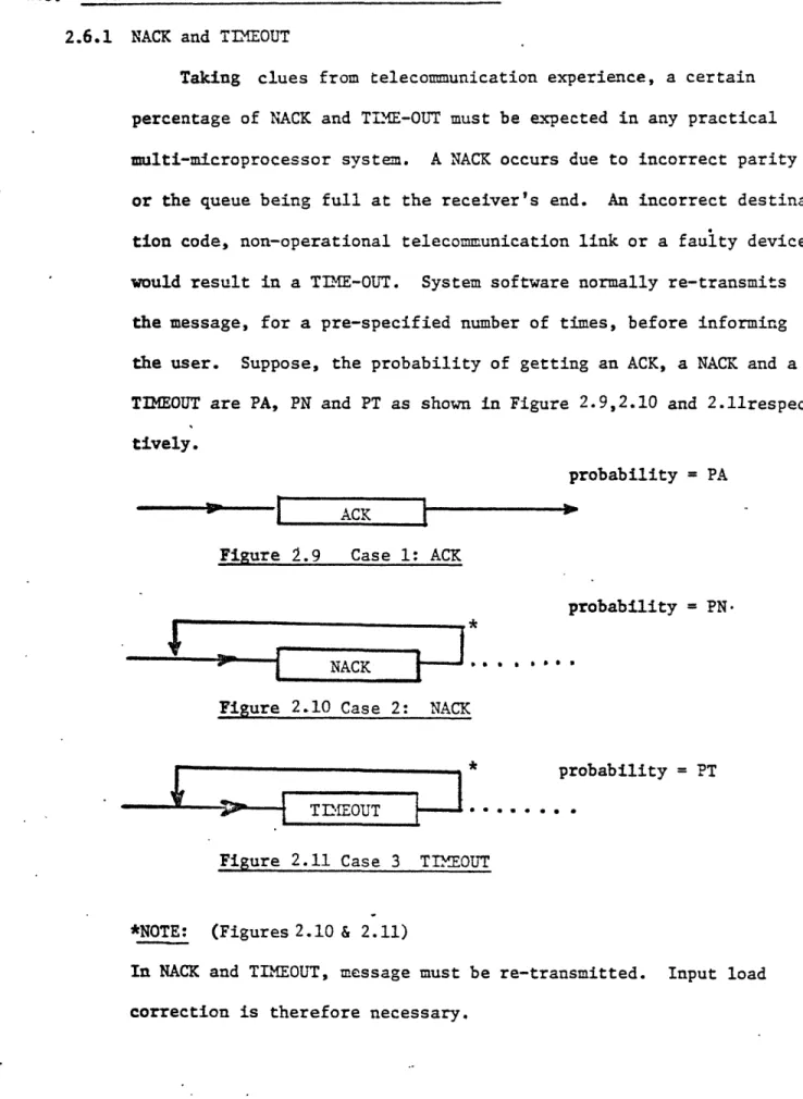
Taking clues from telecommunication experience, a certain

percentage of NACK and TI.ME-OUT must be expected in any practical

multi-microprocessor system. A NACK occurs due to incorrect parity

or the queue being full at the receiver's end. An incorrect

destina-tion code, non-operadestina-tional telecommunicadestina-tion link or a faulty device

would result in a TIME-OUT. System software normally re-transmits

the message, for a pre-specified number of times, before informing

the user. Suppose, the probability of getting an ACK, a NACK and a

TIMEOUT are PA, PN and PT as shown in Figure 2.9,2.10 and

.11respec-tively.

probability = PA

ACK

Figure 2.9 Case 1: ACK

probability =

PN-Figure 2.10 Case 2: NACK

*

probability

=

PT

)> ---

TIMEOUT

**...

Figure 2.11 Case 3 TIMEOUT

*NOTE:

(Figures 2.10 & 2.11)

In NACK

and TIMEOUT, message must be re-transmitted. Input load

correction is therefore necessary.

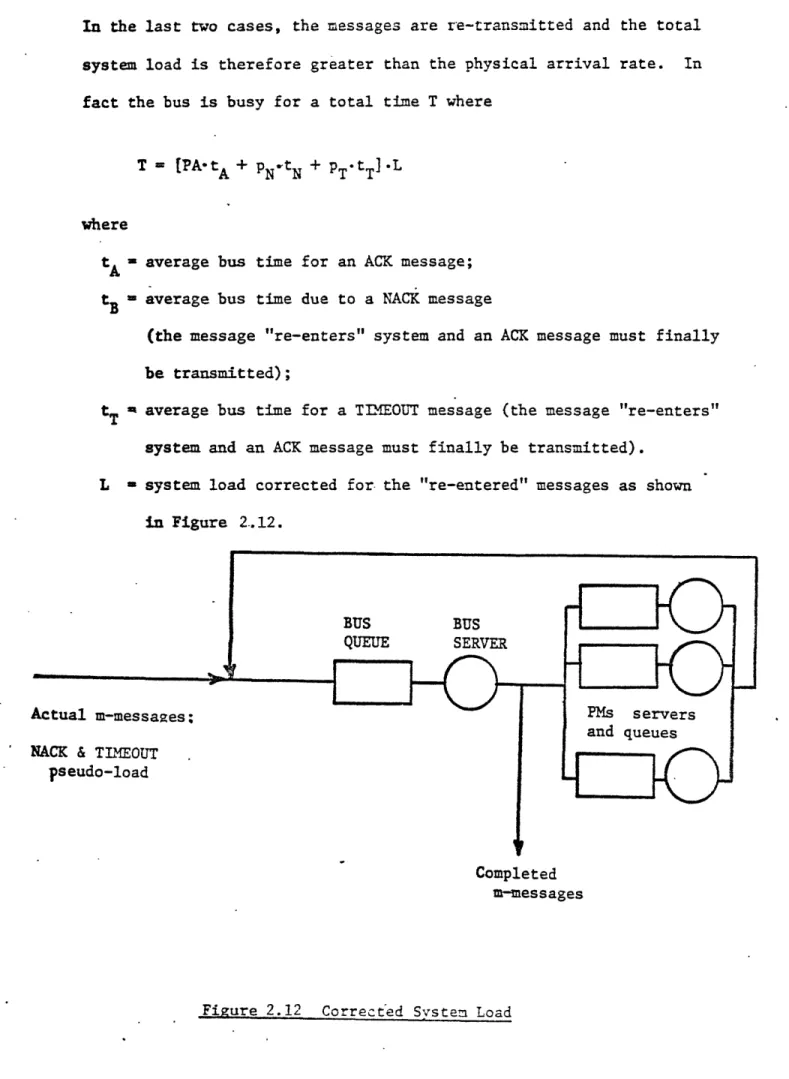
In the last two cases, the messages are re-transmitted and the total system load is therefore greater than the physical arrival rate. In fact the bus is busy for a total time T where

T = [PA-tA + PN-tN + PTLtT] L

where

tA = average bus time for an ACK message; t_B = average bus time due to a NACK message

(the message "re-enters" system and an ACK message must finally be transmitted);

t

T

system and an ACK message must finally be transmitted).

L m system load corrected for the "re-entered" messages as shown

in Figure 2.12.

Completed m-messages

2.6.2 Workload Characterization - An Idealized Case

Consider a multimicroprocessor configuration with 10 processors (PPM) and 10 m=ory units (7PM) all sharing a single bus. For this case assume the memory service time (read/write) is 500 nanoseconds, and the bus service time is 100 nanoseconds. Assume that each processor makes 1.4 accesses to memory every microsecond, and all memory units are used equally on the average (i.e. a uniform distribution of processor requests

to the 10 memories - Figure2.13.

In the specific case described above, there are 1.4 messages per pro-cessor per microsecond, or a total of (1.4 messages/propro-cessor/microsecond) X (10 processors) X (106 microsecond/second) = 14 X 106 messages per second.

Using traditional methods of memory access, each message keeps the memory

busy for (1 bus service time + 1 memory service time + 1 bus service time)

= (100 ns + 500 ns + 100 ns) = 700 ns. Using values of service time and message arrival rate, DILMS analysis indicates that the bus utilization

exceeds 97%, causing an average wait time exceeding 12 microseconds, and the

response time for each memory access of almost 13 microseconds.

The same workload was next analyzed, with the aid of IMMPS, in a~ Pended Transaction environment (5). In this case, the m-message consists of the following:

(i) An e-message from processor to memory

- bus service time of 100 ns;

(ii) Actual memory access

- memory service time of 500 ns;

(iii) An e-message from memory to processor

- bus service time of 100 ns.

IMPS generated the following results:

(i) Response time for first e-message (ii) Memory response time

(iii) Response time for reply e-message Total time for transaction Bus Utilization = 119.23 ns = 537.31 ns = 119.23 a 775.77 ns = 27.78%

Td9-

9J--WTTL

I18-

_li-

_z

N11

0,

Li-z

~i*--·~-l·~·~~·~

0

~---It is seen that for the particular datapoint assumed, the Pended Transaction protocol drastically reduces the response time (from 13 microseconds to less

than 1 microsecond) and the bus utilization from 97% to 28%.

It is fairly simple to include the impact of NACK and TlIMEOUT on the system behavior. Assume that there is a 1% probability of NACK and TI-MOUT each. One can then create dummy messages with a frequency of 1% of actual messages, (1% of 14 X 10 messages/second or 0.14 X 106 messages/second), and

these messages have a bus service time equal to the ACK service time, or a different service time depending on how the system hardware and software behave when an abnormal condition is detected.

2.6.3 Workload Characterization - Another Case

In the previous sub-section, specific values of service times and transaction rates were assumed. These values are dictated by the system architecture and the particular job environment. Here, we consider a more realistic case.

The future will witness increased usage of speech recognition and voice answer back systems. Consider the system in which speech inputs are used as commands/queries to a data base, and the answers are "spoken" by the.computer, followed by a prompt to the user for the next question. In a distributed system, the configuration may be as depicted in Figure 2 .14. In this case, the maximum data input and data output rates are less than 8 KB/sec each. The total load on the bus is 16 KB/sec. If the same data base were now to be accessed by say 60 users simultaneously (e.g. airline reservations or auto-mated bank tellers), there will be a worst case of 60 such loads of 16 KB/sec. Knowing the bus service time and disk service time, all input parameters for an IMMPS analysis are now available and could be used to evaluate the

performance of different communication protocols.

At MIT, IIMPS has been used to study several multimicroprocessor appli-cations likely to become widespread by the late eighties.

2.6.4 Homogeneity Assumption

A final INMPS consideration must deal with the time-history dependence of m-messages. In several instances, the nu-'er cf --messages, or t*e i~nut queries, is not an autonomous variable, but is dependent directly on the previous' system response. For example, if a bank teller responds after a

VOICE INPUT

8+8

=

16 KB/sec

BUS

8 KB/sec

I

A Typical System

Figure 2.14

wait of one hour, the number of user queries will be much lower than a case where the teller responds in one second. This feedback effect cannot be explicitly accounted for within L'E~ S, but can be indirectly accounted for by considering different time-periods with their own characteristic input loads.

When designing future systems to cater to particular applications, the effort is geared towards identifying system protocols that operate comfortably with the prescribed workloads, and in addition have sufficient margin to cater to incidental overloads. This implies that the response times are within reasonable limits, and the users are able to do their work on an undiminished basis. It is best to consider the maximum transfer rates of peripherals while evaluating the bus loads, as this results in maximum contention and the longest response timings. In such a case, one gets the worst case behavior of the system, irrespective of the heterogeneity of the workload involved.

CHAPTER THREE

APPLICATIONS AND THEORETICAL CONSTRAINTS

3.1 INTRODUCTION

In the preceding chapter, IMMPS was described in some detail, and its relevance for multimicroprocessor system design and evaluation was outlined. While analyzing multimicroprocessor bus architectures,

one is soon confronted with questions realted to the job environment in which these systems are expected to operate. Computer performance evaluation has traditionally classified environments (27) as Scientific (high CPU loads, and negligible Input/Output) or Commercial (low CPU loads, high I/O). The literature generally neglects evaluation of real-time systems altogether. The future will witness new uses of the computer technology, such as in areas of speech recognition, audio response, word/graphics processing and real-time movies. For such applications, the simple categories of Scientific versus Commercial are neither pertinent nor useful. Instead, from the vast continuum of applications, one identifies discrete applications to serve as benchmarks in the design and evaluation process. In this chapter, four discrete application reference points are identified and described.

To the above "primal" problem, the "dual" aspect is equally important. One doesn't wish to reinvent the wheel, if some previous wheel can serve the purpose, possibly with sor.e modifications. In

the case of computer communications, the Synchronous Data Link Communication (31) has been in usage for some time, and it would be pertinent to evaluate the efficacy of SDLC for the particular

appli-cations. In (5), an innovative parallel bus has been outlined, and this PENDED architecture is also evaluated in this thesis. Finally, a leading computer manufacturer has come up with another parallel bus that bears at least some resemblence to PENDED; this design is codenamed "Q" in this thesis.

In this chapter, we focus on the theoretical capacities of

"Q", PENDED and SDLC bus architectures. The efficiency or suitability of any bus architecture is usually examined in terms of the actual throughput and response timings. In the ideal case, the messages will not be required to wait, and the response time will equal the service

time. Also, if one can control the actual arrival time of all individual messages, the bus can be loaded continuously, or the bus utilization

increased to one. In such a case, the bus throughput is implicitly dependent on the protocol overhead and the data transfer data. It is obvious that any real life situation will yield throughput lower than the maximum under the ideal conditions enunciated above. One must therefore undertake a deeper analysis only if the "maximum throughput" is at least adequate for the intended application.

3.2 Datapoints

The adequacy angle raises the implicit question of "adequate for what?" In [17], the analysis was focused around a graphic display application

(I,

0-CL.

LL)

u11 CO

L1

co

TOTAL DATA LOADS ON BUS FOR VARIOUS DATAPOINTS

DATAPOINT 1

COMM, -- FLOPPY

_{125 KB/S}

FLOPPY

-

TEXT

₄₀

KB/S

TEXT

--

GRAPHICS

GRAPHICS

->DISPLAY

40

KB/S

-75

KB/S

KEYBOARD

PRINTER

NEGLIGIBLE

280

KB/S

FIGURE

3.1

(B)

280 Kilobytes per second.

Figure 3.2 depicts a text scrolling application, and the total data transfer rate is now about 10.7 Megabytes per second. Figure 3 .3 shows a configuration similar to Figure 3.1, but with additional capaLilities for speech recognicion and voice answer back; the data transfer rate aggregates to 1.7 Megabytes per second.

Finally, in Figure 3.4, we have the real time color movie. Assuming that a single memory contains all the data, the total bandwidth requirements

are now 47.3 Megabytes per second.

The four applications described above are used as the data reference points for calibrating the response times possible through implementing the alternative bus architectures.

3.3 THEORETICAL CONSIDERATIONS

For each of the various bus architectures ("Q", PENDED and SDLC)

there is a definite upper bound to the data transfer rate that can be sustained under the most ideal conditions. This upper bound is determined by circuit

speeds, the width of the data transfer path, and the implicit overheads inherent in flags and arbitration. In this section, these upper-bound values are

determined as a function of the message size. 3.3.1. "0"

At the present time, the message size has no known bounds, and several possible cases are therefore considered. In case only one data byte is

transferred per message, the actual message size is 3 frames with the first two frames being header frames, followed by the data frame. Including arbitra-tion, the transfer time, or the time for which the bus is unavailable to

others, is about 1.33 microseconds. Hence, the maximum data transfer rate

equals:

i data s :z= eiessuae = 0.75 Megabytes/second

u ci CN 4-Ln

C1D

I--DATAPOINT 2

TEXT/IFAGE PROCESSOR

MEMORY <-> DISK

3.95

MB/S

MEMORY .-- > DISPLAY

3.95 MB/S

MEMORY --

TEXT/IM!AGE

OTHERS

2,5

MB/S

NEGLIGIBLE

10,4

MB/S

FIGURE 3 2

(B)

=3= LL CLLJ + >-LU -4 0- i-+ v, l--0~ n-t-<1

_rg

c•

PI

DATAPOINT 3

TEXT

EDITOR WITH SPEECH RECOCNITIOV- VOICE ,ANSWER

BACK

4

DATAPOINT 1

+

ADDITIONIIAL DATA LOAD OF 1,5 MB/S

S

1,

7

-

1,8

MB/S

s=

6 TIMES THE LOAD OF DATAPOINT I

U NT V3

*

DATAPOINT 4

REAL TIME MOVIE COLOR

*TOTAL LOAD

47,3 MB

TO SUMMARIZE:

D

₁

D

₂

D

₃

D

₄

= 0,280

= 10.4

S1,7

=

47,3

MB/S

MB/S

MB/S

MB/S

FIGURE

3

.4

(B)

If 8 bytes are transferred every time, the message size equals

8 bytes + 2 = 6 frames, and the transfer time is 2.33 microseconds, giving

2

a maximum data transfer rate equaling 8 data bytes/,essage = 3.4 Megabytes/sec. 2.33 microseconds/message

The maximum data transfer rates for longer messages are similarly calculated, and the results are summarized in Figure 3.5. It is readily observed that the maximum bandwidth of the "Q" protocol ranges from 0.75 Megabytes/second. 6.0 Megabytes/second depending on the message size.

3.3.2Pended

Here, it takes 50 nanoseconds to transfer a message frame four bytes of address information. The remaining 2 bytes of the first frames, and all four bytes of the second and all subsequent frames, carry data (in block transfer mode).

If a message consists of one data byte only, only one message frame is necessary. The transfer time being 50 nanoseconds, the maximum data transfer rate is 20 Megabytes/second.

If, however, the message is comprised of eight databytes, three message frames are necessary. The transfer time is now 3 x 50 nanoseconds = 150 nanoseconds, giving a maximum data transfer rate equaling

8 databvtes/message = _{53.3 Megabytes/second}

150 nanoseconds/message

With similar calculations for longer messages, one obtains the results summarized in Figure 3.6. The Pended bus architecture permits a maximum data transfer rate varying between 20 Megabytes/second and 80 Megabytes/second depending on the message size.

4

5,

3-MESSAGE

(LOG

SCALE)

FIGURE

3,5

5,5

No, OF I

NEGABYTi

(THEORE-6 MB/s

3,43

512

SIZE

- -

C

---

-

---· *~---- -- -~·P---·

- -- 7--- ---

~

NO, OF DATA

BYTES/SEC.

(THEORETICAL)

5M

79M

53M

20M

512

MESSAGE SIZE

(LOG SCALE)

PENDED

FIGURE 3,6

80

.60

40

20

B0M

IE ~- I--- --~L --- -~ I~IPBPI~ · ·- ·---

240K

200K

160K-

-80K-

40K-1

8

64

512

co

MESSAGE SIZE

(LOG

SCALE)

FIGURE 3,7

SDLC

I

Z~I

3.4 SU•cMMARY

In Section 3.2, the total communication loads for each of the four applications were calculated to be as follows:

Datapoint 1 = Datapoint 2 = Datapoint 3 = Datapoint 4 =

In Section 3.3, the maximum capacities itectures was shown to be as follows:

PENDED = SDLC = 0.28 MB/sec 10.7 MB/sec 1.7 MB/sec 47.3 MB/sec

of the three bus

arch-6 MB/sec 80 MB/sec

0.278 MB/sec

Thus, in the "best" case, "Q" can accomodate datapoints 1 and 3 only, and SDLC is incapable of handling any of these applications. In the next chapter, the impact of contention is studied using LMMPS, and expected values of response times obtained.

LUAkIL1K tuULK: tLUZIt ii'11NC5

4.1 Introduction

Response time is the sum of service time and the wait time. As message

size increases, the service time increases proportionately. However, for

the same data rate, there are now fewer messages, and a corresponding decrease

in the probability that two messages will arrive simultaneously or almost

simultaneously. This decreases the wait time. Thus, the overall response time

reflects two conflicting trends, and it is advantageous to identify the

minima in the curve; this point gives "best response time", and a realistic

throughput rate.

In this section, IIMPS is used to calculate the response time.

4.2

"Q"

We

assume an M/C/1 model, i.e., an exponential distribution of the

message arrival rates, and a constant service time, with a single central

server. The analysis is made for different message sizes (databytes per

message

=

1, 8, 64 and 512).

Further, the impact of increasing the bus

speed by factors of 10 and 100 respectively, is evaluated for the same

message sizes. The increase in the bus speed can be due to one or both

of the following reasons:

(a)

Using a faster technology for implementing the

bus structure;

(b)

Using multiple (but identical)

"Q"

buses to

interconnect all the elements.

In case (b), one must realize that such multiple buses require more buffer

areas in all elements; furthermore, the housekeeping overhead for splitting

the message for transmission purposes, and for the subsequent message

recreating (or concatenation) exercise, will be enormous.

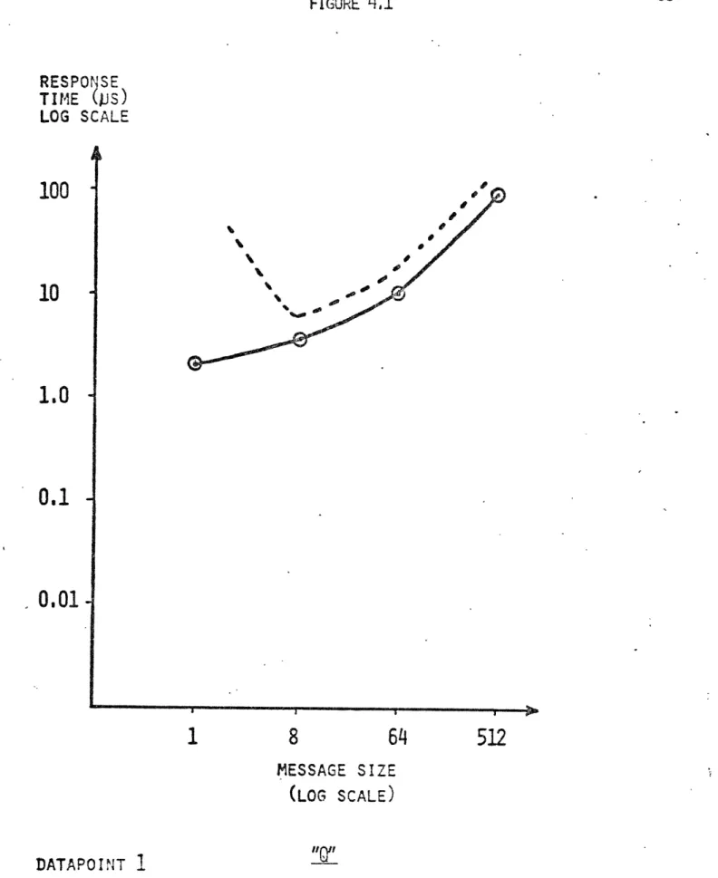
The results for the four datapoints are contained in Tables 4.1 and

4 .2.; these are summarized in Figure 4.1. It is seen that the present

"Q"

speeds permit direct implementation for datapoint

1,

and possibly

for 3. The other datapoints dictate a

modification

of the "present" "Q"

RESPOMSE TIr'E

( )

=

DATAPOINT

I

FACTOR

100

0.01332

SPEED

10

0,136

0,234

(0.284)

1,169

(1,304)

8,62

(9.523

TABL 4,1

WITH

( ) =

DATAPOINT

2

(Js)

BUS

1

1,725

(oo)

2,433

(co)

(0.01436)

0,024

(0,025)

0.116

(0,117)

0.86

(0,87)

64

11.979

(co)

512

88,157

BLOCK

SIZE

WITHOUT

TABLE

.2

RESPOINSE

TITIE

(Cus)

IQT

BUS

1

SPEED

10

0.152

(Co)

3,435

(co)

14.290

(w)

103.28

(ce)

0.238

(co)

1.184

(5.089)

8,73

(25.6)

BLOCK

SIZE

WITHOUT

( )

=

DATAPOINT

₃

(

)

=

DATAPOINT

4

FACTOR

100

0.014

(0,025)

0.023

(0.025)

0.1168

(0.112)

0.86

(0.8)

512

WITH

FIGURE 4.1

RESPONSE

TIME (JS)

LOG SCALE

64

MESSAGE SIZE

(LOG SCALE)

DATAPOINT

1

2 &

4 (DOTTED

3

(DOTTED

LINE)

100

10

1.0

0.

-

0.01-512

~--

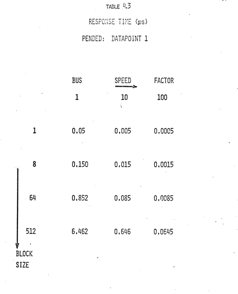
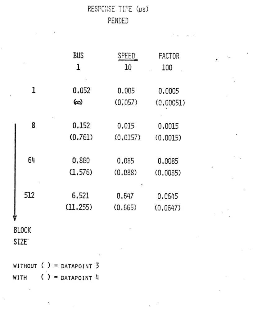
4.3 Pended

The Pended bus architecture described in (5) is also modeled for various message sizes (1, 8, 64 and 512 data bytes per message), with bus speed factors of 1, 10 and 100, all under M/C/1 conditions. The results for the four data-points are shown in Tables 4.3, 4.4 and 4.5; the graphical summary is con-tained in Figure 4.2. It is seen that the Pended protocol can cope

with all the different data loads, except that a real time movie isn't feasible with a message size of 1 byte/frame.

4.4 SDLC

SDLC has several options, namely Point to Point, Loop and Multipoint configurations (31) . In point to point, each processing element is arranged as shown in Figure 4.3 for datapoint 1.

CONMM . FLOPPY a•0 TEXT GRAPHICS - DISPLAY

125 KB/s 40 KB/s 40 KB/s 75 KB/s Figure 4.3: SDLC Point to Point

In a general case with 'n' processing elements, and each PE directly connected to every other PE, 'n x n' linkages will be necessary. As value of n increases, this option becomes increasingly unattractive, from the cost viewpoint.

The Loop is constrained by the limitation that in order to communicate with another secondary PE, a secondary PE must first transfer the entire message to a primary, and then another message is transmitted to the (destination) PE.

FLOPPY

TEXT

TABLE

4.3

RESPON:E

_{TIT'E (Ns)}

PENDED: DATAPOINT 1

SPEED

10

0.005

0.015

0.085

0.646

BUS

1

0.05

0.150

0.852

6,462

FACTOR

100

0,0005

0,0015

0.0085

0.0645

64

512

BLOCK

SIZE

TABLE L 4

RESPONSE TIE

(.us)

PENDED: DATAPOINT 2

SPEED

10

0.006

0.016

0.0856

0

,E49

BUS

1

0,075

0.168

FACTOR

100

0,0005

0,0015

0.0085

0,064

5

64

0.919

512

6.943

BLOCK

SIZE

I

TABLE 4,5

RESPONSE

TNDE

(Ds)

PENDED

BUS

1

0.052

wo)

0,152

(0.761)

0,860

(1.576)

6.521

(11.255)

SPEED

10

0.005

(0;057)

0,015

(0,0157)

0,085

(0.088)

0.647

(0.665)

FACTOR

100

0,0005

(0.00051)

0,0015

(0.0015)

0,0085

(0.0085)

0.0645

(0.0647)

WITHOUT ( )

=

DATAPOINT

₃

WITH

(

)

=

DATAPOINT

4

64

512

BLOCK

SIZE'

FIGURE

4

.2

RESPONSE TIME (US)

LOG SCALE

100

10.0

1.0

0.1

0,01

64

MESSAGE SIZE

(LOG SCALE)

PENDED

DATAPOINT

1

2

AND

3

ALMOST COINCIDE WITH

1

4

(AS DOTTED LINE)

-P

512

%

I, o 0

--· I~8ba

TABLE 4.6

RESPONSE TIN-E

(ps)

SDLC

SPEED

10

5,733

-(3.147)

27.13

(26.07)

212.499

FACTOR

100

0.264

(0.259)

0.514

(0.511)

12.564

(2.556)

20.112

WITHOUT (

) =

MULTIPOINT

(

)

=

POINT TO POINT

WITH

t

NO.

OF BYTES OF INFORMATION

4

NO, OF MESSAGES

RESPONSE TIME FOR EVEN THE

LONGER MESSAGE

BUS

1

(04

8

64

512

(146)

(443)

BLOCK

SIZE

TAB•L

4,7

RESPONSE

lE

(Tli•

s)

SDLC

SPEED

10

co

c*ae

(oo)

FACTOR

100

(0,351)

1,029

(0,540)

3.471

(2.643)

26.981

(20,714)

T

BLOCK

SIZE

WITHOUT

( ) =

DATAPOINT

2

WITH

( )

= DATAPOINT

3

RESPONSE TIME FOR DATAPOINT 4 IS

oo

IN

ALL CASES,

BUS

1

@0)

64

@o)

512

m)

Ir

FIGURE

RESPONSE TIME (PJS)

LOG

Sf

100

10

1.0

0.1

-0.01.

CALE

MESSAGE SIZE

(LOG SCALE)

SDLC

(X 10)

DATAPOINT

1,

2,3,4

(cH

64

512

Further, none of the links can be full duplex. Thus the 40 KB of data load

between TEXT and GRAPHICS results in 40 KB of load from TEXT to CCMM and

another 40 KB from COMM to GRAPHICS. In all, it represents an average load

of more than 40 KB for each link in the loop. The aggregate load of 280 KB/sec

thus reflects almost 340 IB/sec over the link between DISPLAY and COMM. On

the whole, this SDLC configuration results in large overheads, and hence

large response times.

The multipoint configuration with full duplex links has been considered

as

it gives "best" response times. The same methodology and datapoints were

used, and the results are contained in Tables .6

and .7.

It is seen that

SDLC, in the present form, is unable to handle the individual loads of any of

the four datapoints at any message size. A bus speed factor improvement of

10 (either by increasing circuit speed, or by using 10 parallel SDLC links)

makes some configurations feasible, and the results are summarized in Figure

.5. Thus, if SDLC is to be used for supporting multimicroprocessor systems;

it must either by speeded up, or a number of parallel SDLC links used; in the

latter case, the inherent overhead must be taken into account.

4.5 CONCLUSION

The data presented in the preceding section can be summarized as shown

below:

BUS STRUCTURE

Datapoint

Datapoint

Datapoint

Datapoint

1

2

3

4

"Q"

Feasible

Not

Feasible

Not

Feasible

Feasible

PENDED

Feasible

Feasible

Feasible

Feasible

SDLC

Not

Not

Not

Not

Feasible

Feasible

Feasible

Feasible

The above matrix illustrates that drastic modifications in SDLC speeds and/

or protocols will be necessary in order to adapt it for multimicroprocessor

applications. The

"Q"

_{protocol is currently suitable for a limited set}

of applications. The PENDED bus protocol

is most suitable for the

multimicroprocessor job environment.

CHAPTER FIVE VALIDATION OF ID S

5.1 INTRODUCTION

In Chapter 2, the IM1PS analytic model was described; operating details are summarized in the appendix to this thesis. This model was used to derive the results in the preceding chapter. In the ideal case, one would have desired to cross-check the results using actual hardware and software. But since all the applications outlined are future projections, and the "Q" and PENDED bus architectures are still being implemented, one is compelled to look for alternative methods for model validation.

IMMPS is based on queueing theory, and the program implicitly uses closed form analytic expressions derived from the concepts of work flow and steady state considerations. Unfortuantely, queueing theory provides results only for systems with static message arrival rates and service times. No doubt for these simple cases, it provides accurate results with little effort. But some inherent assumptions of queueing theory are not exactly valid, in particular, the

assump-tion about infinite queue capacities. However, if physical queue capacities are more than 10 times the value of expected queue length, the queue capacity can be assumed to be infinitely long for all practical purposes. In Chapter 2, this approximation error was shown to be

But to a critical observer, more direct evidence is required to completely validate the queuing model. An excellent analysis of these issues is contained in (32).

Fortunately, Abdel-Hamid (19) has developed simulation models for bus architectures. These simulation models, programmed in GPSS, have been used to verify the results obtained with I`MfMPS. Since the GPSS models assume finite queue capacities, it is possible to evaluate the true impact of assumptions made in ITMPS. (It would be relevant to point out, however, that a simulation run for a few milliseconds of real time costs more than 10,000 times as much as the execution of an equivalent analytic model in terms of computer time. Thus, some restraint in the domain of simulation runs became essential.)

5.2 RESULTS FROM THE TWO MODELS

For "Q" bus architecture, and datapoints 1, 2 and 3, the results

are summarized in Tables 5.1, 5.2 and 5.3 respectively. The results for PENDED are contained in Tables 5.4, 5.5 and 5.6 (21).