HAL Id: hal-00557553
https://hal.archives-ouvertes.fr/hal-00557553
Submitted on 19 Jan 2011
HAL is a multi-disciplinary open access
archive for the deposit and dissemination of
sci-entific research documents, whether they are
pub-lished or not. The documents may come from
teaching and research institutions in France or
abroad, or from public or private research centers.
L’archive ouverte pluridisciplinaire HAL, est
destinée au dépôt et à la diffusion de documents
scientifiques de niveau recherche, publiés ou non,
émanant des établissements d’enseignement et de
recherche français ou étrangers, des laboratoires
publics ou privés.
Smart range finder and camera fusion - Application to
real-time dense digital elevation map estimation
C. Debain, F. Malartre, P. Delmas, Roland Chapuis, T. Humbert, M.
Berducat
To cite this version:
C. Debain, F. Malartre, P. Delmas, Roland Chapuis, T. Humbert, et al.. Smart range finder and
camera fusion - Application to real-time dense digital elevation map estimation. Robotics 2010,
International workshop of Mobile Robotics for environment/agriculture, Sep 2010, Clermont-Ferrand,
France. p. - p. �hal-00557553�
Smart Range Finder and Camera Fusion - Application to Real-Time
Dense Digital Elevation Map Estimation
Christophe Debain*, Florent Malartre**, Pierre Delmas*, Roland Chapuis**, Thierry Humbert* and Michel Berducat*
*Cemagref, UR TSCF, 24, avenue des Landais, BP 50085, 63172 Aubi`ere, France
(e-mail:[email protected])
**LASMEA - UMR 6602, 24, avenue des Landais, 63177 Aubi`ere, France
Abstract—This paper is about environment perception for
nav-igation system in outdoor applications. Unlike other approaches that try to detect an obstacle of binary state, we consider here a Digital Elevation Map (DEM). This map has to be built in regards to the guidance system’s needs. These needs depend on the vehicle capabilities, its dynamics constraints, its speed etc... Starting with the navigation system’s needs, our goal is to estimate a precise and dense DEM. Our approach is based on a SLAM algorithm combining a one map rangefinder and a camera. Thus we can estimate both the displacement between two laser scan and have a good density of the reconstructed DEM. The approach has been validated both using simulated realistic data and in real conditions with our robot in outdoor environement. The estimation of the DEM has been done successfully in real-time (approx. 40ms per loop).
I. INTRODUCTION
The design and the conception of mobile robots in highly unstructured outdoor environments as agricultural applications is still an open issue. Many teams in the world are working on this subject addressing different research domains. [9] introduces the difficulties encountered when autonomy is given to a vehicle which has to move in real contexts. Lots of scientific problems have to be considered in this huge subject as perception of the environment [4], control in difficult situation like sliding terrain [3] with stability constraints [2], obstacle avoidance [10]... All these subjects are essential and have to be considered in an elegant manner in order to be efficient and reliable. Since 2004, our team decided to address these problems from a new point of view. Since the beginning of the robotic domain, the most part of the research teams have considered the robotic problems from the sensors point of view. For instance, usually when we want to localise a robot, we use a sensor like a GPS (global localization) or a camera (local localization) and a fusion is achieved. Then, powerful algorithms need to be developed to extract features and the result is the input of the control algorithm in order to automatically drive vehicles.
In our case, we consider the autonomy of the robot and we try to model what is useful for this autonomy. For automatic guidance it means that we should try to extract data in order to optimize a criterion that takes into account the required precision, the needed integrity, safety ... For instance, in our work on the SLAG concept (Simultaneous Localization And Guidance), we show that the perception system can stop to work if the guidance conditions are fulfilled [19]. The main
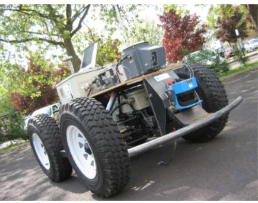
idea in this concept is to call a resource (sensor or algorithm) when it is necessary evaluating the ratio between gain and cost of each resource. If all the needs of the robot are fulfilled, no resource are called. This concept has been use for the first time in [18] to automatically guide a vehicle (see figure 1) and no ”obstacle notion” was considered [6], the automatic adaptation to different context and the reliability of the demonstration were particularly appreciated.
In our current works we want to apply this concept to insure the physical integrity of the robot. More precisely the goal to reach is to ensure the vehicule has the capability to cross the ground in front it, in a given corridor. Il this application, the system requires the ground geometry in a dynamic zone (depending on its speed, and the wished navigation corridor). The purpose of this paper is to obtain the Digital Elevation Map (DEM) in real-time with a good accuracy. In the proposed approach this area is obtained using both a camera and a laser scanner coupled in a SLAM process. The guidance system will therefore searches for the most optimal path in regards to the criteria of stability and speed.
Obtaining a DEM is fairly easy if we use dense data sensors (such as a Velodyne, for example). If we use more con-ventional sensors (such as camera and classical rangefinders) obtaining the DEM is much more difficult.
Using a single camera, although, seems attractive in terms of implementation and cost issues. Nevertheless major problem occur: density of the DEM, stability problems, drift and scale ratio in usual SLAM technics.
To stabilize the solutions, the approach suggested here combines two sensors: a camera and a lidar in a single SLAM process. To reach this goal, the wished analysis area is back-projected in the image frame with a flat-ground assumption. The region of interest obtained is divided into a large number of points (usually a few hundreds). The one map laser scanner provides a dense set of 3D points in front of the vehicle (at approximately a 5m distance). These points are tracked in the image in a SLAM process in order to obtain iteratively a dense DEM. Depending on the needs of the the guidance system, points can be added and tracked between each laser scan to fill the lack of data.
The paper is organized as follows: first, we present classical approaches in section II. In section III, our approach is presented and the main parts of the system is exposed. We will show the obtained results with our approach in section
Author-produced version of the paper presented at Robotics 2010, International workshop of Mobile Robotics for environment/agriculture Clermont-Ferrand, France, 3-4 sept 2010
Fig. 1. The vehicle AROCO
IV. Finally, conclusions and future works will be addressed in section V.
II. RELATED WORKS
A. Obstacle detection
Usually, obstacles detection is based on detecting and clas-sifying them with binary state: safe, unsafe. In [14], authors describe how to segment stereo pictures and decide what is an obstacle and what is not. This segmentation does not rely on the vehicle’s dynamical constraints and so may be unusable depending on vehicle state (a small stone may not be an obstacle at low speed, but can be at high speed). The same comments can be done for [15] where authors interpret pic-tures from monocular camera to find obstacles after a learning process. All those methods rely on data interpretation and/or 2D 1/2 representation to perceive potential obstacle. On the other hand, for the vehicle safety and if we consider optimal path generation, a 3D representation of the environment is more suitable for the navigation system. Therefore, a DEM is considered to be able to find best path according to both dynamics and integrity constraints of the vehicle.
B. Digital Elevation Map
In order to obtain the optimal path, we need a 3 dimension-nal representation of the environment to satisfy the guidance system. It is also important to know the uncertainty on this 3D representation to choose the safest path. For example, the guidance system could make a mistake if it is detecting a flat ground with a big uncertaincy that can affect the physical integrity of the vehicle. The localization of the mobile robot on this map must also be considered for the control system and to chose an optimal path. In this paper, we will consider the world as static. Therefor, moving object are not considered here.
C. Vision-only Digital Elevation Map
Many researchers work on the DEM estimation problem using stereo-vision, optical flow, etc (for example see [1]). In outdoor conditions, dense stereo approaches are not well suited because of the baseline required to obtaine good re-sults. Optical flow approaches are rather restricted to obstacle movements rather than ground reconstruction.
Fig. 2. Unobservability of the rangefinders
Nowadays a popular method is the Simultaneous Localiza-tion And Mapping approach (SLAM) which consists in finding the pose of the vehicle and building a map in the same process [11, 7, 5]. If we consider vision-only SLAM, the main problem is that visual features used for the process are usually extracted from remarkable points (Harris points [8] or SIFT [12]). Therefore the elevation map could have a lack of information big enough to make the guidance system fail between these remarkable points. In fact it is really necessary to control the amount of data to perceive from the environment in order to fulfill the needs of the guidance system. On the other side, the control system must adapt itself if our perception system can’t provide enough accurate data (due to a lack of computation time or insufficient sensor accuracy).
A solution coming up is to use stereo pair camera to build the elevation map in the SLAM process. The problem remains that the accuracy of far points is dependant of the stereo baseline. The accuracy is also influenced by the good calibration of the cameras.
D. Lidar-only Digital Elevation Map
Besides the high cost 3D laser scanner solutions a few works use one map scanners. Indeed, having only one scan does not give the whole map in front of the robot. Nevertheless, it is still possible to build a DEM using a one map rangefinder. For example, consider the vehicle is equiped with a Lidar inclined to look at the ground. We make the assumption that this mobile robot is perfectly localised (Position and Orientation). Consequently we are able to build the DEM as long as the vehicle moves. Obviously, the granularity of the reconstruction depends on the vehicle speed. The space between two acquisitions can be modulated if we control the speed. But the faster we move, the more accurate map we need. The consequence is that if we want to go fast, we cannot because we have a large unobserved space between two rays proportional to the vehicle speed (fig. 2).
E. Our approach
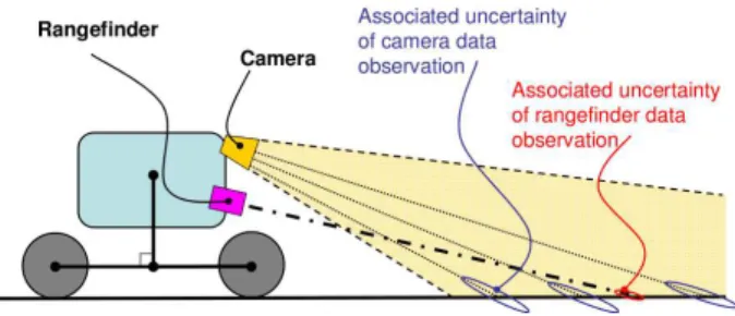
In conclusion, using a rangefinder alone is not sufficient (even a 3D rangefinder) because the quantity of information is not sufficient and not controllable. But a camera can provide high density data on demand. On the other hand, a rangefinders is usually used on mobile robot for safety (detecting pedestrians for example). This paper proposes a method to combine the accurate data from the rangefinder with the dense and controllable data from a camera in a SLAM process.
Fig. 3. Camera and rangefinder sensors fusion
III. VISION-LIDAR FUSION
A. Introduction
In this section, we present our method to efficiently build a DEM flexible enough to fit the guidance needs. An Extended Kalman Filter will be used. Our method consists in combining the 3D data provided by the lidar to the corresponding points in the image in a SLAM process. We propose to observe the rangefinder points in the camera in order to have both an accurate estimation of the 3D environment (for the DEM) and an observation of this environment in the camera (for the localization). The camera informations are used to extend our world perception thanks to the high density of information it gives. Figure 3 shows the system.
Here the difficulties are due to the projection of the 3D points on the camera being non-remarkable since we wish the guidance to control the data density and not the environment. The technics used in the state of the art to track points in pictures flow are not usable here because authors try to matches points extracted from the environment as being remarkable points. Therfore, we have developed algorithms able to track common points in picture giving a patch and a region of tracking. Usually the points we track come from a laser scan: their 3D position is therefore known with a low uncertainty (assuming calibration stage has been done previoulsy between camera and laser scanner, see III-E). Since most of the points come from a laser scan, the SLAM stability is very high and it is possible to reconstruct points out of the laser scan to fill the DEM in wished positions.
Notice we only use a subset of the points given by the laser scanner (usually 30). We will see later that all the scanner points will be used to compose the dense MAP (see section III-F).
B. Problem formulation
First, the state vector of our system is composed of 6 parameters of the vehicle pose Xv= (X,Y, Z,α,β,γ)T plus
3 parameters per points of our local map Xp= (xp, yp, zp)T,
p ∈[1, n] which give the state vector (1).
X= (XTv, XT1, · · · , XTn)T= (X,Y, Z,α,β,γ, x1, y1, z1, . . . , xn, yn, zn)T (1) n represents the number of points necessary to fullfil the guidance system’s needs depending on its dynamical con-straints (speed, vehicle caracteristic ...). The calculated points
are initialized into the focus area provided by the application. The 3D points initilization will be done as follow:
• m< n points will be initialized with the informations
coming from the Lidar. We can found the 3D coordinates of the rangefinder’s 2D points in the camera’s frame using the transition matrix PL−C. Determination of the
PL−C matrix will be done in section III-E. This matrix
is used to transfer the points from the lidar frame to the camera frame. The uncertainty associated is given by the rangefinders manufacturer (a few centimeters). Those points will be refered as lidar points.
• l= n − m points will be initialized in the world frame
to fill the focus area of the guidance system. Their initialization will be made assuming they are on the ground and with a certain uncertainty (typically 0.5m). Those points will be refered as camera points.
Thanks to the rangefinder, the initial state of the EKF is very close to the real state and its covariance is low for lidar points. These conditions will guaranty a good convegence of the filter. The EKF needs to have access to the equation of the state evolution and the state observation. In our case, the observation is given by the projection of the state points in the camera’s frame (u, v). To update the state vector we also need the
jacobian matrix of those equations.
These equations and their respective jacobian matrices are given in [13]. The next step will be to update the state vector X for each time t.
C. Global method v.s Point to Point method
Our objective is to estimate the whole state vector X for each time t. We assume we are able to track nt≤n points Xi
of the state vector in the next image using a patch (recorded in the previous image or when we added this point in the state vector) in a small traking area (deduced, as usual, from the covariance of the vehicle state estimation). This gives us observation sets (ui, vi)T with (i ∈[1, nt]) to feed the SLAM
process.
However the EKF can be processed in two different ways: (1) we can feed the filter with all the data we got in the current image and (2) we can provide only one observation at a time and repeat the process for all the data.
The first method (described in Algorithm 1 and referenced as GM) have some drawbacks. In this case, the size of the tracking region is constant and used for every points. That means that we cannot focus our attention taking account succesfull matches and the signal noise ratio won’t be optimal. Thus the probability for a false positive match is increased. We also have to deal with the inversion of a 2nt×2ntmatrix where
nt is the number of points from the state vector sucessfully
matched. This inversion is very time consuming.
On the other hand algorithm (2) is described in Algorithm 2 and refered as PTPM. In thois case, we see that the size of the tracking region is given by the current observation covariance. The first point wil make the process converge and the area of interest for the nexts points will be drastically reduced in size. Thus, we have a size of tracking region which is focused after
Algorithm 1 SLAM global method: GM
1: Prediction of the state evolution.
2: Compute the observation jacobian.
3: Compute the observation covariance.
4: Tracking of state points observed in the image flow.
5: Compute the observation jacobian in regards to the points succesfully tracked.
6: Update the EKF with the innovation.
Algorithm 2 SLAM Point to Point method: PTPM
1: Prediction of the state evolution.
Require: nt = Number of tracked points
2: for i= 1 to nt do
3: Compute the observation jacobian.
4: Compute the observation covariance.
5: Track the point in the image flow.
6: Update the EKF with the innovation.
7: end for
each iteration of the EKF (but we have nt iterations for a given image). The benefit are both in computation time and rejection of false positive matchings. Furthermore, unlike the first method we only have to compute nt 2 × 2 matrices (the
computational times are approximately divided by nt).
Those two methods are currently implanted on our software architecture. This paper will also compare results for the two methods.
D. Unsynchronized data
We have now all the equations to implement the EKF for our Vision-Rangefinder system.
However we also need to fill our state vector with data’s from the rangefinder. For this, we have to project data from the rangefinder frame in the camera frame and acquire patches on the image where the laser impact occures (to be observed sev-eral times). The problem is that the data from the rangefinder are not synchronized with the camera’s pictures (see fig.2)
Thanks to the previous work in our lab.[17] we can recover an optimal state vector at the desired date. In this case we use a spline interpolation of the 6 parameters of the localization to retrieve the camera position and orientation at the rangefinder date.
Once the position of this camera is found, the transition matrix P(C
[L−date]−C[C−date]) has to be computed. This matrix projects points of camera frame at rangefinder’s date to the nearest (in acquisition time) valid camera frame. A valid camera frame is a frame where a picture has been acquired.
The equation to project rangefinder points XL to a valid camera frame Xc is given by eq.(2).
Xc= P(C[L−date]−C[C−date]) PL−CXL (2) At this moment, the points can be added to the state vector with an initial covariance. Finaly we have described how to add points in the state vector. Together with the EKF equations
Time C1 C2 R1 C3 x z x z x z x z x z C1 C2 C3 R1 Spline interpolation
?
Fig. 4. Interpolating the Rangefinder position and orientation in the ’nearest’ camera frame.
Fig. 5. The pattern used to calibrate the camera-rangefinder system
and the main algorithm to be processed we now have all informations and steps to perform our SLAM process. E. Calibration of a Camera-Rangefinder set
In section III we saw that a transition matrix is needed in order to use the rangefinder points in the camera. This transition matrix is simply a 4 × 4 matrix composed of 3 rotations and 3 translations. We have used software already developped in our laboratory. The principle is described in [16] even if we envizage to use more recent methods (such as [20]) in near future. To achieve the extrinsic calibration we use an orthogonal pattern (Figure 5).
The vehicle moves forward to the pattern and a dataset composed of camera picture and rangefinder scan is acquired. The camera dataset is used to compute the position and orientation of the camera in the pattern mark (PP−C). Then
the rangefinder dataset and the vehicle trajectory are used to compute the position and orientation of the pattern in the rangefinders frame (PL−P). The calibration matrix is then
simply deduced using eq. (3).
PL−C= PL−PPP−C (3)
F. Dense Digital Elevation Map
The presented SLAM is able to compute a large list of 3D points in real-time (about 150). But this is usually insufficent for the guidance process which needs a map of about one thousand points to evolve at a raisonnable speed (2 m/s). Thus
Fig. 6. Internal view of the experimentation. Our vehicle AROCO in a real outdoor environment. On the left : the camera picture with projected state points. On the right : the DEM.
we have to gather a more dense DEM. This task is easily obtained thanks to the rangefinder. Even if all the rangefinders points have not been used in the SLAM process, they can be used to fill the DEM because of their good accuracy. To do this, we simply have to put the rangefinder slices in the estimated position frame thanks to equation 4. Then, we have to use all our 3D points (from rangefinders and from SLAM) to fill the DEM in accordance to the guidance process needs (density, observation range and length). For points in the DEM not been observed by the rangefinder, we still have enough computation time to include regular camera points in the SLAM process and estimate them.
XDEM= P(C[L−date]) PL−C XL (4) Therefore the DEM can be estimated in a local frame at the date wanted by the guidance process. In the following section we will present the results obtained with our approach.
IV. RESULTS
In this section, we present the results of the DEM estimation based on our camera and rangefinder fusion. The comparison will be made between the two algorythms presented in this paper (GM and PTPM, see section III-C). First, in order to quantify the reconstruction errors, we will use a simulator we have developped. Notice we have made two movies1showing (1) the real-time behaviour of our method (algorithm PTPM) implemented in real-time on our robot (see figure 1 and figure 6) and (2) the behaviour using our simulator (real-time implementation) where a similar vehicle evolves in a simulated environment. The vehicle is equiped with a pinhole camera (resolution of 800x600) and a rangefinder inclined to look at the ground (impact at about 3 meters on flat ground). The frequency of our camera is set to 25 Hz and the frequency of the rangefinder is set to 12.5 Hz. Our vehicle is moving at about 1.5 m/s. The simulated vehicle is equipped with the
same sensors as the real one. We drove the vehicle (both in simulation and real case) manually and, in the simulated case, the reconstructed DEM is compared to the ground truth provided by the simulator.
1http://www.lasmea.univ-bpclermont.fr/ ftp/pub/chapuis/ICARCV2010 −1 −0.5 0 0.5 1 0 1 2 −0.1 0 0.1 0.2 Z (m) X (m) Y (m) 0 0.2 0.4 0.6 0.8 1 1.2 1.4 1.6 1.8 2 −0.03 −0.02 −0.01 0 0.01 0.02 Y (m) Z (m)
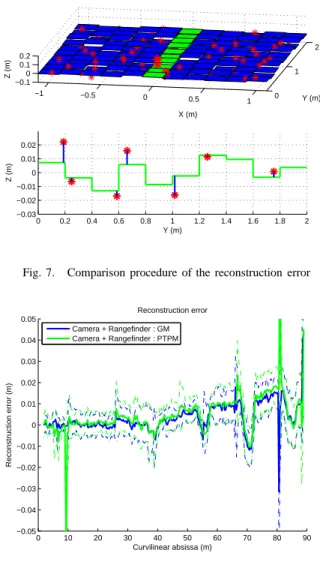
Fig. 7. Comparison procedure of the reconstruction error
0 10 20 30 40 50 60 70 80 90 −0.05 −0.04 −0.03 −0.02 −0.01 0 0.01 0.02 0.03 0.04 0.05 Reconstruction error Reconstruction error (m) Curvilinear absissa (m) Camera + Rangefinder : GM Camera + Rangefinder : PTPM
Fig. 8. Mean and Standard Deviation of the reconstruction error
A. DEM estimation
In this case, we compare the reconstructed points coming from the state vector to the ground truth given by the simulator that provides an elevation grid of the environment in front of the vehicle (5x5 meters large). After each iteration, point’s height of the state vector are compared with the elevation grid. We have acquired a data set which will be used for both algorithms.
Fig. 7 shows the comparison procedure whereas fig. 8 reports the reconstruction error in height of the state points for the whole experimentation (100m long: see movie1). Fig. 9 shows the global world map reconstructed at the end.
The difference with the real simulated world comes from the drift of localization (the world in our simulator is very flat but SLAM is very sensitive to this: a much more complicated world would give better drift).
Concerning the real exprimentation (see movie), the cali-bration matrix PL−Cfrom the rangefinder to the camera frame
has been extracted as mentionned in this paper. The experi-mentation shows the vehicle moving on an environment over a
Fig. 9. The world built by our system. −2 0 2 4 6 8 10 12 14 0 10 20 30 40 50 60 70 80 90 Environment map Ground Truth Camera + Rangefinder : GM Camera + Rangefinder : PTPM
Fig. 10. Trajectory reconstruction between slam estimation and the ground truth (Top view).
100 meters long trajectory (Fig. 10). The DEM reconstruction is shown in the Digital Elevation Map window in the video. This window represents a top view of the 3D points in the local frame. Points shown in green levels are points near the ground (ie. ±10cm). Points in red or blue levels are points respectively higher and lower than the ground.
B. SLAM localization evaluation
Fig. 10 represents a top-view of the followed trajectory with all trajectories computed by our methods (in the simulation case). The error of localization is reported in fig. 11. Similar results are obtained in real situation (see [13]).
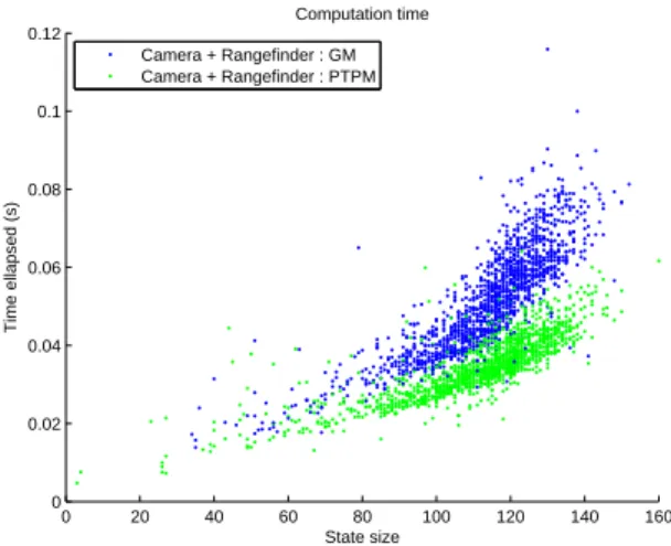
We can see that we are able to follow that kind of trajectory with our camera and rangefinder fusion with a very small drift. All those results in this paper have been processed in real-time with a C++ software [17]. The computation real-time in regards to the number of points is represented in Fig. 12. As expected, the PTPM method is performed faster than the GM method. For exemple, computation time for the whole EKF process includind tracking is tipicaly 40ms for 130 points with the PTPM method (State vector of size 396). This software is independant of the data used (simulation or real experimentation). 0 10 20 30 40 50 60 70 80 90 0 0.1 0.2 0.3 0.4 0.5 0.6 0.7 0.8 0.9 1 Localization error Localization error (m) Curvilinear absissa (m) Camera + Rangefinder : GM Camera + Rangefinder : PTPM
Fig. 11. Trajectory error between slam estimation and the ground truth.
0 20 40 60 80 100 120 140 160 0 0.02 0.04 0.06 0.08 0.1 0.12 Computation time State size Time ellapsed (s) Camera + Rangefinder : GM Camera + Rangefinder : PTPM
Fig. 12. Computation time of the whole process. Global method and Point per Point method.
V. CONCLUSIONS AND FUTURE WORKS We have presented an efficient method to recover a dense elevation map whose density could be easily controllable. Our system can satisfy the guidance process goal by controlling the amount of data reconstructed. This need must be taken in account if we want to achieve the automatic guidance whatever the evolution speed is. In this paper, we proposed a SLAM based system combining a laser scanner and a camera. The obtained system is able to provide a DEM of hundreds points to fill the guidance needs with good stability. Two methods have been presented, the PTPM method showed slightly better results than GM method with a smaller computation time. The dense Digital Elevation Map is recovered thanks to the rangefinder and the 6 parameter localization provided by our system.
Those solutions has been implanted in real time on a common laptop configuration and has been demonstrated on both realistic simulated configuration and on our real robot at approximatively 2m/s speed. Depending on the application
needs, it would be straighforward to work at high speeds (5 to 10 m/s). A future step will be to check unobserved space of the map and to fill them with camera’s point estimated with our SLAM (since we still have enough computation time). Finally, our next step will be to combine this intelligent environment perception with an attentional control system. This will allow the vehicle to move at an optimal speed taking into account both its dynamic and its perceptive capabilities.
REFERENCES
[1] Francisco Bonin-Font, Alberto Ortiz, and Gabriel Oliver. Visual navigation for mobile robots: A survey. J. Intell. Robotics Syst., 53(3):263–296, 2008.
[2] N. Bouton, R. Lenain, B. Thuilot, and P. Martinet. A rollover indicator based on a tire stiffness backstepping observer: Application to an all-terrain vehicle. In Intelli-gent Robots and Systems, 2008. IROS 2008. IEEE/RSJ International Conference on, pages 2726–2731, Sept. 2008.
[3] C. Cariou, R. Lenain, B. Thuilot, and P. Martinet. Adaptive control of four-wheel-steering off-road mobile robots: Application to path tracking and heading control in presence of sliding. In Intelligent Robots and Systems, 2008. IROS 2008. IEEE/RSJ International Conference on, pages 1759–1764, Sept. 2008.
[4] F. Chanier, P. Checchin, C. Blanc, and L. Trassoudaine. Map fusion based on a multi-map slam framework. In Multisensor Fusion and Integration for Intelligent Sys-tems, 2008. MFI 2008. IEEE International Conference on, pages 533–538, Aug. 2008.
[5] Javier Civera, Oscar G. Grasa, Andrew J. Davison, and J.M.M. Montiel. 1-point ransac for ekf-based structure from motion. In Proceedings IEEE/RSJ Int. Conf. on Intelligent Robots and Systems (IROS), St. Louis, October 2009.
[6] P. Delmas, N. Bouton, C Debain, and R Chapuis. Envi-ronment characterization and path optimization to ensure the integrity of a mobile robot. IEEE International Conference on Robotics and Biomimetics (ROBIO 09), 2009.
[7] J. Diebel, K. Reutersward, S. Thrun, J. Davis, and R. Gupta. Simultaneous localization and mapping with active stereo vision. In Intelligent Robots and Systems, 2004. (IROS 2004). Proceedings. 2004 IEEE/RSJ Inter-national Conference on, volume 4, pages 3436–3443 vol.4, 2004.
[8] C. Harris and M. Stephens. A combined corner and edge detection. In Proceedings of The Fourth Alvey Vision Conference, pages 147–151, 1988.
[9] Alonzo Kelly and Anthony (Tony) Stentz. Minimum throughput adaptive perception for high speed mobility. In Proceedings of the IEEE/RJS International Conference on Intelligent Robotic Systems, volume 1, pages 215 – 223, September 1997.
[10] O Khatib. Real-time obstacle avoidance for manipulators and mobile robots. Int. J. Rob. Res., 5(1):90–98, 1986.
[11] T. Lemaire, Cyrille Berger, I-K. Jung, and S. Lacroix. Vision-based SLAM: stereo and monocular approaches. International Journal on Computer Vision, 74(3):343– 364, 2007.
[12] David Lowe. Object recognition from local scale-invariant features. pages 1150–1157, 1999.
[13] F. Malartre, T. Feraud, C. Debain, and R. Chapuis. Digi-tal elevation map estimation by vision-lidar fusion. IEEE International Conference on Robotics and Biomimetics (ROBIO 09), 2009.
[14] R. Manduchi, A. Castano, A. Talukder, and L. Matthies. Obstacle detection and terrain classification for au-tonomous off-road navigation. Auton. Robots, 18(1):81– 102, 2005.
[15] Jeff Michels, Ashutosh Saxena, and Andrew Y. Ng. High speed obstacle avoidance using monocular vision and reinforcement learning. In ICML ’05: Proceedings of the 22nd international conference on Machine learning, pages 593–600, New York, NY, USA, 2005. ACM. [16] P. Pujas and M.J. Aldon. Etalonnage d’un systme de
fusion camra-tlmtre pour la fusion multi-sensorielle. In AFCET RFIA’96, 1996.
[17] C. Tessier, C. Cariou, C. Debain, R. Chapuis, F. Chausse, and C. Rousset. A real-time, multi-sensor architecture for fusion of delayed observations: Application to vehicle localisation. In 9th International IEEE Conference on Intelligent Transportation Systems, pages 1316–1321, Toronto, Canada, September 2006.
[18] C. Tessier, C. Debain, R. Chapuis, and F. Chausse. Fusion of active detections for outdoor vehicle guidance. In Information Fusion, 2006 9th International Conference on, pages 1–8, July 2006.
[19] C. Tessier, C. Debain, R. Chapuis, and F. Chausse. A cognitive perception system for autonomous vehicles. In Cognitive systems with Interactive Sensors (COGIS), Stanford University California USA, 26/11/07-27/11/07, 2007.
[20] Qilong Zhang. Extrinsic calibration of a camera and laser range finder. In In IEEE International Conference on Intelligent Robots and Systems (IROS, page 2004, 2004.