HAL Id: cea-02564098
https://hal-cea.archives-ouvertes.fr/cea-02564098
Preprint submitted on 16 Dec 2020
HAL is a multi-disciplinary open access
archive for the deposit and dissemination of
sci-entific research documents, whether they are
pub-lished or not. The documents may come from
teaching and research institutions in France or
abroad, or from public or private research centers.
L’archive ouverte pluridisciplinaire HAL, est
destinée au dépôt et à la diffusion de documents
scientifiques de niveau recherche, publiés ou non,
émanant des établissements d’enseignement et de
recherche français ou étrangers, des laboratoires
publics ou privés.
distribution of population in China
Jiachen Ye, Qitong Hu, Peng Ji, Marc Barthelemy
To cite this version:
Jiachen Ye, Qitong Hu, Peng Ji, Marc Barthelemy. The effect of interurban movements on the spatial
distribution of population in China. 2020. �cea-02564098�
Jiachen Ye,1,2 Qitong Hu,1,2 Peng Ji,1,2∗ and Marc Barthelemy3,4†
1Institute of Science and Technology for Brain-Inspired Intelligence, Fudan University, Shanghai 200433, China
2
Research Institute of Intelligent and Complex Systems, Fudan University, Shanghai 200433, China
3
Institut de Physique Théorique, Université Paris Saclay, CEA, CNRS, F-91191 Gif-sur-Yvette, France and
4
Centre d’Analyse et de Mathématique Sociales, (CNRS/EHESS) 54, Boulevard Raspail, 75006 Paris, France (Dated:)
Understanding how interurban movements can modify the spatial distribution of the population is important for transport planning but is also a fundamental ingredient for epidemic modeling. We focus here on vacation trips (for all transportation modes) during the Chinese Lunar New Year and compare the results for 2019 with the ones for 2020 where travel bans were applied for mitigating the spread of a novel coronavirus (COVID-19). We first show that these travel flows are broadly distributed and display both large temporal and spatial fluctuations, making their modeling very difficult. When flows are larger, they appear to be more dispersed over a larger number of origins and destinations, creating de facto hubs that can spread an epidemic at a large scale. These movements quickly induce (in about a week) a very strong population concentration in a small set of cities. We characterize quantitatively the return to the initial distribution by defining a pendular ratio which allows us to show that this dynamics is very slow and even stopped for the 2020 Lunar New Year due to travel restrictions. Travel restrictions obviously limit the spread of the diseases between different cities, but have thus the counter-effect of keeping high concentration in a small set of cities, a priori favoring intra-city spread, unless individual contacts are strongly limited. These results shed some light on how interurban movements modify the national distribution of populations, a crucial ingredient for devising effective control strategies at a national level.
I. INTRODUCTION
In early January 2020, we observed the outbreak of a novel coronavirus (COVID-19) in Wuhan, China, which has been quickly spreading out to the whole country, and more recently to other countries in the world [1]. In-fectious diseases spread among humans because of their interactions and movements, and the proximity of this outbreak with the Spring Festival, a period of travel with high traffic loads, provided terrible conditions for the spread of this disease. With an increasing amount of confirmed cases, more attention has been devoted to modeling the spread of COVID-19 from various aspects such as determining the value of the reproductive number [2–7], of the incubation period [8–10]. In general, analyt-ical modeling plays of course an important role in the prediction of the spread and allows in particular to test control strategies [11], which was verified in this case too [12–20, 20, 21, 21, 22]. Particularly important were esti-mate of probability to export the disease in other coun-tries [19, 23, 24], and how effective were travel restrictions inside China [19].
Demographic information and mobility, either under the form of data or given by transportation models (see for example the review [25]), are crucial for these trans-mission models. Mobility can concern either the global scale with movements between countries [18–21], or the national scale between cities, or even inside cities [20–22].
∗Electronic address: pengji@fudan.edu.cn †Electronic address: marc.barthelemy@ipht.fr
In this study we are focusing on the national level and we won’t try to model the spread of the disease. Instead we will focus on the statistical properties of the interur-ban mobility, and how it affects the spatial distribution of populations. More precisely, we will investigate the statistical properties, of traffic flows between cities dur-ing the Chinese Sprdur-ing Festival in 2020 and by compardur-ing with data for 2019, which are the most salient differences induced by travel restrictions. This knowledge will help us to understand the effect of travel restrictions and their impact on epidemic spread, and more generally to guide us for modeling mobility at this scale, a crucial ingredient in epidemiological studies, but also for other fields such as transportation planning.
II. STATISTICS OF INTERURBAN FLOWS
We will first study standard statistical properties of in-terurban flows obtained from migration data collected by Baidu Qianxi (see Material and Methods). This dataset enables us to monitor the traffic flows between cities. For each day d (d = 1, 2, . . . , T ), we can extract the number of individuals N (i, j, d) going from city i to city j with any travel mode. The migration data can thus be seen as a directed, weighted network of flows between the set of n = 296 cities of China whose populations are also known (see Material and Methods). We collected the data for the Spring Festival of 2020 (from Jan. 1st to Feb. 12th, 2020) and for assessing the impact of travel bans, we also collected the data for the Spring Festival of 2019 (which according to the Chinese lunar calendar takes place from Jan. 12th to Feb. 23rd, 2019).
Figure 1: (a) Distribution of all traffic flows N (i, j, d) in
loglog. The line is a power law fit of the form N−α with
exponent α = 2.27 with fitting method described in [26]. (b) Average and standard deviation of the flows N (i, j, d) aver-aged over traffic flows versus the date d (from 1st January to 12th February).
Large heterogeneity of flows
We first consider the distribution of all flows of in-dividuals N (i, j, d) for all cities i and j and all days d and which is shown in Fig. 1 (a). The maximum flow is of order 105 and the average of order 103 indicating
a broad distribution. A power law fit is consistent with this picture with an exponent α ≈ 2.3 (Fig. 1 (a)). This heterogeneity is confirmed in Fig. 1 (b) which shows both the average value µdand the standard deviation σd
com-puted over all inter-city flows (for each day d). We see that for most days the relative dispersion σd/µd is of
or-der 5 − 10. This heterogeneity is probably due to the large diversity of cities that can serve as origins or des-tinations of flows (see below for further analysis). An important feature that we can observe on Fig. 1 (b) is the sharp drop of the standard deviation after Jan. 25th, the Lunar New Year (LNY), which we will see below is mainly due to the travel ban (see also Fig. S1, S3 in SI for a detailed discussion).
Temporal versus spatial fluctuations
In order to understand the nature of the different fluc-tuations affecting the flows N (i, j, d), we compute the relative standard deviation ∆ij= σµij
ij, where µij and σij
are the average and standard deviation computed over
Figure 2: (a) Relative standard deviation of the flows N aver-aged over traffic flows and represented here versus time. (b) Distribution of the relative standard deviation of N averaged
over time. (c) Relative standard deviation of Nin(i, d) and
Nout(i, d) averaged over cities and shown here versus time.
(d) Distribution of the relative standard deviation of Ninand
Noutaveraged over time
time, and the relative standard deviation ∆d =σµdd,
aver-age over all flows, for a given day d. We show on Fig. 2 (a) the spatial dispersion ∆d versus time and in Fig. 2
(b) the distribution of ∆ij. We observe that the spatial
dispersion is of order 8.3, while the temporal dispersion is less (mainly concentrated around 1). The main reason for heterogeneity thus lies in the flow fluctuations between different origins and destinations, while temporal fluctu-ations are smaller but not negligible. These two sources of heterogeneity clearly represent a challenge for model-ing these flows, especially with very simplified models. Our results indicate that the first modeling step would be to describe the spatial heterogeneity of flows and then consider temporal variations.
The next natural quantities that can be computed over this network are the incoming and outgoing flows defined by ( Nin(i, d) =P n j=1N (j, i, d) Nout(i, d) =P n j=1N (i, j, d) (1) respectively. We measure in the same way as above var-ious measures of fluctuations, either averaged over cities or over time, leading to the quantities ∆in (out)d , ∆in (out)i . As these quantities are sums of random variables, we ex-pect smaller relative dispersions than for N (i, j, d) which is indeed what we observe (see Fig. 2 (c) and (d), with typical values of relative dispersion of order 1 (see Figs. S4,S5 for additional details). In order to get first insights about the influence of travel bans, we compare the in-coming flows and outgoing flows versus city population in 2019 and 2020 with days Nbefore
in, out before and Nout,inafter
after LNY. We first observe that (see Fig. S2 in Supple-mentary Information (SI)) basically the number of out-going individuals before LNY corresponds approximately
to the number of incoming individuals after LNY with Nbefore
in (out) ≈ N after
out (in) (and vice-versa). These relations
thus correspond roughly to the conservation of the num-ber of individuals traveling during the Chinese Spring Festival.
Structure of incoming and outgoing flows
The value of incoming or outgoing flows gives infor-mation about the volume of migrations, but not about the number of important origins or destinations. In or-der to characterize the dispersion over different cities, we denote by O(i, d) and D(i, d), the sets of origin of flows incoming in city i and destinations of flows from city i (for the day d), respectively. We then use Gini indices [27] that capture the dispersion of incoming and outgoing flows and are given by
Gin(i, d) = 1 2O2N in(i, d) X p,q∈O(i,d) |N (p, i, d) − N (q, i, d)| (2) Gout(i, d) = 1 2D2N out(i, d) X p,q∈D(i,d) |N (i, p, d) − N (i, q, d)| (3) where O and D represent the number of elements of the sets O(i, d) and D(i, d). The quantity Nin(i, d) = N|O(i,d)|in(i,d)
is the average incoming flows and Nout(i, d) =
Nout(i,d)
|D(i,d)|
the average outgoing flows. Intuitively, if all traffic flows to city i are from one single origin city on day d, the Gini index Gin(i, d) will be 1, while if traffic flows to city i are
all equal, the Gini index Gin(i, d) will be 0 (and similarly
for Gout(i, d)).
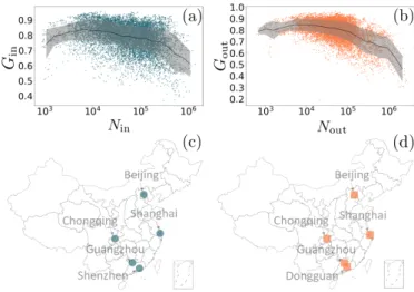
We plot these Gini indices computed for each city ver-sus the traffic flows to or from this city. These figures 3 (a,b) show that on average the larger the traffic flows are, the more dispersed they are over a larger number of origins or destinations. In terms of epidemic control, it is clear that cities with a large flow Ninand a small Gini
index Gin are the most critical, in the sense that many
people from many different cities are converging to the same place. Equally, cities with a large Nout and a small
Goutshould be particularly monitored, since they can act
as hubs in spreading the disease over the inter-city net-work. As shown in Fig. 3 (c,d), we show the top 5 crit-ical cities, including Beijing, Shanghai, Chongqing and Guangzhou for both the incoming and outgoing flows, Shenzhen for the incoming flows, and Dongguan for the outgoing flows.
III. STATISTICAL STRUCTURE OF THE
NATIONAL POPULATION
An important effect of incoming and outgoing flows is that they change the population structure. Some cities
Figure 3: (a) Ginversus Nin for all cities and days. (b) Gout
versus Nout for all cities and days (shown in loglog). The
thick line indicates the average of Gin ( Gout ) versus of Nin
(Nout) and the shaded area represents the standard deviation
of the average. Top 5 critical cities for (c) incoming flows and (d) outgoing flows.
will receive a large number of individuals while for others we expect a decrease of their population. Migration thus affects the statistical structure of the national population and in this section we will characterize this effect.
Temporal evolution of population structure
In order to characterize the disparity of the population distribution and how it varies during seasonal migrations, we consider the population of city i at time d given by
P (i, d) = P0(i) + X d06d Nin(i, d0) − X d06d Nout(i, d0), (4)
where P0(i) represents the population of city i without
incoming and outgoing flows. The Gini index for the city population of the whole country at day d is then given by G(d) = 1 2n2P (d) n X i,j=1 |P (i, d) − P (j, d)|, (5) where P (d) = n1Pn
i=1P (i, d) is the average population
of all cities at day d. Intuitively, if all people gather in one city, G will be 1, while if people spread evenly across all cities, G will be 0. For comparison, we also define the Gini index at rest as
Grest= 1 2n2P 0 n X i,j=1 |P0(i) − P0(j)|. (6)
This quantity captures the degree of population con-centration without any traffic flows, where P0 =
Figure 4: Temporal variations around the Spring Festival hol-idays of the population Gini index for 2019 and 2020. The horizontal dotted line represents the value ‘at rest’. The ver-tical line indicates the day of the LNY.
1 n
Pn
i=1P0(i) is the average population of all cities
with-out any traffic flows. We show in Fig. 4 the variation of the Gini coefficient when we take into account mi-gration flows. We plot both the results for 2019 and 2020. In both cases we see an important increase of the Gini coefficient in a short time (about a week): when the LNY is approaching, people go back from workplaces to hometowns for reunion with families. A smaller set of cities concentrates these meetings with the number of im-portant cities reaching its minimum and the Gini index reaching its peak on the LNY. Based on the Gini index, we can estimate the number of ‘important’ cities where the concentration takes place through [n(1 − G)], where [·] denotes the integer part (see SI for details where we show in Fig. S6 this number versus time and we indeed observe an important drop when approaching the LNY). After the LNY (Jan. 25th), individuals are going back home and the Gini coefficient relaxes back to its origi-nal value, but much slower. We observe that in 2020, the increase of the Gini index is larger and, due to travel bans, the decrease even slower than normal. The rea-son may be that after the outbreak of COVID-19, almost all regions have deferred the time of resuming works and classes after the Spring Festival holiday. For example, Shanghai proposed that companies not crucial to the na-tion should not resume works before Feb. 10th and that schools should provide online classes. At this point, the population structure at the national level is far from be-ing back to normal. These different results show that these seasonal movements induce a strong concentration of individuals in a relative small set of cities, and that travel bans tend to keep this situation of high concentra-tion.
Return to ‘equilibrium’: pendular ratio
We observe in Fig. 4 that after the LNY there is a decrease of the Gini index indicating a return to normal
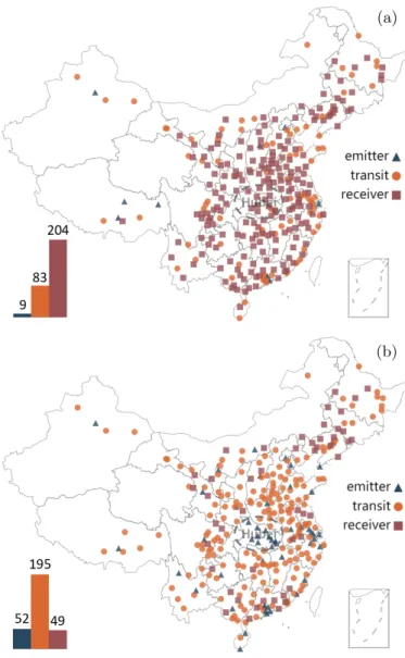
Figure 5: (a) Emitter, receiver and transit cities according to the value of R(i, 1) for 2019 with the number of three cate-gories of cites at lower left corner. (b) Emitter, receiver and transit cities according to the value of R(i, 1) for 2020 with the number of three categories of cites at lower left corner.
state characterized by a lower concentration of individu-als. In order to characterize quantitatively this return to the original state (before holidays), we measure the gap between individuals going out from a city before the LNY and coming back after it. This gap defines a ‘pendular ratio’ given by R(i, df) = P ˆ d<d6 ˆd+dfNin(i, d) P ˆ d−df6d< ˆdNout(i, d) , (7)
where df is a range of days around the LNY ˆd. If this
ratio is much larger than 1, it means that for this city there is a large incoming flow while for the opposite sit-uation R(i, df) 1, a large number of individuals are
going out (compared to the incoming flows). At large times df, we expect that R ' 1 since most of the
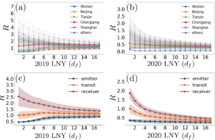
in-Figure 6: Comparison of pendular ratio between 2019 and
2020. (a) Pendular ratio for all cities versus days df from
LNY in 2019. We highlight five important cities. (b)
Pendu-lar ratio for all cities versus days df from LNY in 2020 with
highlight of 5 cities. (c) Average values of the pendular ratio over cities according to the classification (receiver, emitter or transit cities) versus days from LNY in 2019. The colored ar-eas correspond to one standard deviation. (d) Mean value of the pendular ratio over cities according to the classification versus days from LNY in 2020 with the shaded area repre-senting the corresponding standard deviation.
dividuals have come back. We divide cities into three categories according to the value of R(i, 1): If the value is larger than 1.5, we classify city i as a ‘receiver’ city. If the value is less than 0.5, we classify city i as an ‘emit-ter’ city. Finally, if the value is between 0.5 and 1.5, we classify city i as a ‘transit’ city. We represent on Fig. 5 the cities of different types on the map of China. We observe that both receiver and transit cities are ho-mogeneously distributed in China. In constrat emitters cities are in general located in developed regions, e.g., Beijing, Shanghai, Guangzhou, and so on, as shown in figures 5 (a) and (b). It is interesting to note that cities of the Hubei province (within the dashed circle in the fig-ure) are emitters cities in 2020, essentially due to travel restrictions that prevented individuals to come back to Wuhan. This is an important difference compared to the year of 2019 that appears here in the spatial structure of emitters and receivers.
We show in Fig. 6 (a,b) the pendular ratio for 2019 and 2020 for all cities and we highlight 5 cities: Wuhan, Bei-jing, Tianjin, Chongqing and Shanghai, corresponding to the origin place of COVID-19 and four province-level mu-nicipalities. We note here that the curve corresponding to Wuhan is at the bottom of all cities in Fig. 6 (b), re-flecting the success of sealing off Wuhan from all outside contact to stop the spread of the disease since Jan. 23rd. In Fig. 6 (c,d) we show this pendular ratio for 2019 and 2020 for the different types of cities (we average over cities in a given category, emitter, receiver or transit). We observe that the standard deviation is small for the three
groups adding credit to their definition. In addition, com-pared to 2019, the values of R(i, 1) corresponding to 2020 are much smaller. We observe that in 2019, the pendular ratio of all the three types of cities returns to 1, mean-ing that the majority of individuals who went away for the holidays came back. The situation for 2020 is very different with a pendular ratio for all types of cities that converges to a value less than 1 (even less than 0.5), indi-cating that the majority of people who went away for the holidays did not come back yet. This result remains con-sistent with the conclusion of Gini index (Fig. 3) about a larger concentration in cities and the effect of travel bans.
Finally, we note here that we additionally implemented our whole analysis at the province level (see SI) and the results obtained are similar are those obtained at the city level.
IV. CONCLUSION
Our findings thus concern four different aspects. First, the traffic flows between cities are very heterogeneous not only spatially but also from a temporal perspective. Such a large heterogeneity could be induced by both the Spring Festival and the travel ban. Similar results apply also to an aggregated level, i.e. the incoming and outgoing flows for cities also display important heterogeneities. This as-pect is crucial for understanding and modeling epidemic spreading for which we know the importance of hetero-geneity for epidemic spreading on networks [28, 29] and more generally for most processes [30]. We also quan-tify the dispersion of origins/destinations of the incom-ing/outgoing flows showing that for larger flows we have a larger variety of origins and destinations. We also show that during these seasonal migrations of the Spring Festi-val, the national structure of population changes quickly with a larger concentration in a small set of cities. This concentration decays normally in time after the festivi-ties but travel bans slow down this return to the initial state. It is natural to try to stop the geographical spread of the disease by stopping interurban movements, but on the other hand, large concentration in cities can favor the spread at the city level and increase the number of infected cases. This concentration can be compensated by a more important control at the individual contact level which is what was done in cities such as Wuhan. These results are in line with epidemic modeling results [19], where it was shown that travel quarantine is effec-tive only when combined with a large reduction of intra-community transmission. Our results thus highlight the importance of mobility studies for modeling a variety of processes and in particular for understanding and model-ing the spread of epidemics. Effective mitigatmodel-ing strate-gies need to take into account the change of population structure that we exhibited here.
V. MATERIAL AND METHODS Data
We obtained the migration data from Baidu Qianxi (http://qianxi.baidu.com), based on Baidu Location Based Services and Baidu Tianyan, for all transportation modes. It provides the following two datasets: migration index reflecting the size of the population moving into or out from a city/province, and migration ratio capturing the proportion of each origins and destination. We col-lected the data during Chinese Spring Festival period of 2020 (from Jan. 1st to Feb. 12th, 2020). For parallel
comparison, the migration index during the same period of 2019 (re-scaled according to Chinese lunar calendar, from Jan. 12th to Feb. 23rd, 2019) is also used.
In addition to the migration data, we collected the demographic from China Statistical Yearbook (http://www.statsdatabank.com), an annual statistical publication, which reflects comprehensively economic and social development of China. It covers key statis-tical data in recent years at both the city level and the province level. We collected the data of population of 31 province-level regions and 296 city-level regions from China Statistical Yearbook 2019, the latest edition pro-vided.
[1] Hernández JC Wee S, McNeil Jr DG. W.h.o. declares
global emergency as wuhan coronavirus spreads. The
New York Times, 2020.
[2] Zhidong Cao, Qingpeng Zhang, Xin Lu, Dirk Pfeif-fer, Zhongwei Jia, Hongbing Song, and Daniel Dajun Zeng. Estimating the effective reproduction number of the 2019-ncov in china. medRxiv, 2020.
[3] Biao Tang, Xia Wang, Qian Li, Nicola Luigi Bragazzi, Sanyi Tang, Yanni Xiao, and Jianhong Wu. Estimation of the transmission risk of the 2019-ncov and its implica-tion for public health intervenimplica-tions. Journal of Clinical Medicine, 9(2):462, 2020.
[4] Julien Riou and Christian L Althaus. Pattern of early human-to-human transmission of wuhan 2019 novel coro-navirus (2019-ncov), december 2019 to january 2020. Eu-rosurveillance, 25(4), 2020.
[5] Shi Zhao, Qianyin Lin, Jinjun Ran, Salihu S Musa, Guangpu Yang, Weiming Wang, Yijun Lou, Daozhou Gao, Lin Yang, Daihai He, et al. Preliminary estimation of the basic reproduction number of novel coronavirus (2019-ncov) in china, from 2019 to 2020: A data-driven analysis in the early phase of the outbreak. International Journal of Infectious Diseases, 2020.
[6] Sang Woo Park, David Champredon, David JD Earn, Michael Li, Joshua S Weitz, Bryan T Grenfell, and Jonathan Dushoff. Reconciling early-outbreak prelimi-nary estimates of the basic reproductive number and its uncertainty: a new framework and applications to the novel coronavirus (2019-ncov) outbreak. medRxiv, 2020. [7] Juanjuan Zhang, Maria Litvinova, Wei Wang, Yan Wang, Xiaowei Deng, Xinghui Chen, Mei Li, Wen Zheng, Lan Yi, Xinhua Chen, et al. Evolving epidemiology of novel coronavirus diseases 2019 and possible interruption of lo-cal transmission outside hubei province in china: a de-scriptive and modeling study. medRxiv, 2020.
[8] Jantien A Backer, Don Klinkenberg, and Jacco Wallinga. Incubation period of 2019 novel coronavirus (2019-ncov) infections among travellers from wuhan, china, 20–28 jan-uary 2020. Eurosurveillance, 25(5):2000062, 2020. [9] Jonathan M Read, Jessica RE Bridgen, Derek AT
Cum-mings, Antonia Ho, and Chris P Jewell. Novel coron-avirus 2019-ncov: early estimation of epidemiological pa-rameters and epidemic predictions. medRxiv, 2020. [10] Tao Liu, Jianxiong Hu, Min Kang, Lifeng Lin, Haojie
Zhong, Jianpeng Xiao, Guanhao He, Tie Song, Qiong
Huang, Zuhua Rong, et al. Transmission dynamics of 2019 novel coronavirus (2019-ncov). 2020.
[11] H. Heesterbeek, R. M. Anderson, V. Andreasen,
S. Bansal, D. De Angelis, C. Dye, K. T. D. Eames, W. J. Edmunds, S. D. W. Frost, and S. Funk. Modeling infec-tious disease dynamics in the complex landscape of global health. Science, 347(6227):aaa4339–aaa4339, 2015. [12] Ye Liang, Dan Xu, Shang Fu, Kewa Gao, Jingjing Huan,
Linyong Xu, and Jia-da Li. A simple prediction model for the development trend of 2019-ncov epidemics based on medical observations. arXiv preprint arXiv:2002.00426, 2020.
[13] Yu Chen, Jin Cheng, Yu Jiang, and Keji Liu. A
time delay dynamical model for outbreak of
2019-ncov and the parameter identification. arXiv preprint
arXiv:2002.00418, 2020.
[14] Wai-kit Ming, Jian Huang, and Casper JP Zhang. Break-ing down of healthcare system: Mathematical modellBreak-ing for controlling the novel coronavirus (2019-ncov) out-break in wuhan, china. bioRxiv, 2020.
[15] Maimuna Majumder and Kenneth D Mandl. Early trans-missibility assessment of a novel coronavirus in wuhan, china. China (January 23, 2020), 2020.
[16] Zeliang Chen, Wenjun Zhang, Yi Lu, Cheng Guo, Zhong-min Guo, Conghui Liao, Xi Zhang, Yi Zhang, Xiaohu Han, Qianlin Li, et al. From sars-cov to wuhan 2019-ncov outbreak: Similarity of early epidemic and prediction of future trends. CELL-HOST-MICROBE-D-20-00063, 2020.
[17] Jun Li. A robust stochastic method of estimating the
transmission potential of 2019-ncov. arXiv preprint
arXiv:2002.03828, 2020.
[18] Joseph T Wu, Kathy Leung, and Gabriel M Leung. Now-casting and foreNow-casting the potential domestic and inter-national spread of the 2019-ncov outbreak originating in wuhan, china: a modelling study. The Lancet, 2020. [19] Matteo Chinazzi, Jessica T Davis, Corrado Gioannini,
Maria Litvinova, A Pastore y Piontti, Luca Rossi, Xinyue Xiong, M Elizabeth Halloran, IM Longini, and Alessan-dro Vespignani. Preliminary assessment of the interna-tional spreading risk associated with the 2019 novel coro-navirus (2019-ncov) outbreak in wuhan city. Center for Inference and Dynamics of Infectious Diseases, USA. Re-trieved, 8, 2020.
Kam-ran Khan, Zhongjie Li, and Andrew Tatem. Preliminary risk analysis of 2019 novel coronavirus spread within and beyond china, 2020.
[21] Matteo Chinazzi, Jessica T Davis, Marco Ajelli, Corrado Gioannini, Maria Litvinova, Stefano Merler, Ana Pastore y Piontti, Luca Rossi, Kaiyuan Sun, Cécile Viboud, et al. The effect of travel restrictions on the spread of the 2019 novel coronavirus (2019-ncov) outbreak. medRxiv, 2020. [22] Xinwu Qian, Lijun Sun, and Satish V Ukkusuri. Scal-ing of contact networks for epidemic spreadScal-ing in urban transit systems. arXiv preprint arXiv:2002.03564, 2020. [23] Giulia Pullano, Francesco Pinotti, Eugenio Valdano,
Pierre-Yves Boëlle, Chiara Poletto, and Vittoria Colizza. Novel coronavirus (2019-ncov) early-stage importation
risk to europe, january 2020. Eurosurveillance, 25(4),
2020.
[24] Marius Gilbert, Giulia Pullano, Francesco Pinotti, Eu-genio Valdano, Chiara Poletto, Pierre-Yves Boëlle, Eric D’Ortenzio, Yazdan Yazdanpanah, Serge Paul Eholie, Mathias Altmann, et al. Preparedness and vulnerabil-ity of african countries against importations of covid-19: a modelling study. The Lancet, 2020.
[25] Hugo Barbosa, Marc Barthelemy, Gourab Ghoshal, Charlotte R James, Maxime Lenormand, Thomas Louail, Ronaldo Menezes, José J Ramasco, Filippo Simini, and Marcello Tomasini. Human mobility: Models and appli-cations. Physics Reports, 734:1–74, 2018.
[26] Jeff Alstott, Ed Bullmore, and Dietmar Plenz. powerlaw: A python package for analysis of heavy-tailed distribu-tions. Plos One, 9, 2014.
[27] Philip M Dixon, Jacob Weiner, Thomas Mitchell-Olds, and Robert Woodley. Bootstrapping the gini coefficient of inequality. Ecology, 68(5):1548–1551, 1987.
[28] Romualdo Pastor-Satorras and Alessandro Vespignani. Epidemic spreading in scale-free networks. Physical re-view letters, 86(14):3200, 2001.
[29] Marc Barthélemy, Alain Barrat, Romualdo
Pastor-Satorras, and Alessandro Vespignani. Velocity and hi-erarchical spread of epidemic outbreaks in scale-free net-works. Physical review letters, 92(17):178701, 2004. [30] Alain Barrat, Marc Barthelemy, and Alessandro
Vespig-nani. Dynamical processes on complex networks. Cam-bridge university press, 2008.
Appendix A: Supplementary Materials Data for 2019
In order to evaluate the heterogeneity of flows of 2019 with comparison to that of 2020, we use the migration index during the same period of 2019 (re-scaled according to Chinese lunar calendar, from Jan. 12th to Feb. 23rd, 2019), and we would compute the distribution of all flows N (i, j, d), for all cities i and j and all days d, though N (i, j, d) = Nout(i, d) × p(i, j, d). The Chinese Lunar New Year of 2019 is Feb. 5th. Here, Nout(i, d) is migration index
reflecting the size of the population moving into or out from a city/province, and p(i, j, d) is migration ratio capturing the proportion of each origins and destination. However, the migration ratio is unavailable for 2019. We apply the data of p(i, j, d) for 2020 to the computation of N (i, j, d) for 2019, with results shown in Fig. S1. This result exhibits large heterogeneity of flows and displays a localized drop around LNY.
Statistics of Nin and Nout
Versus population
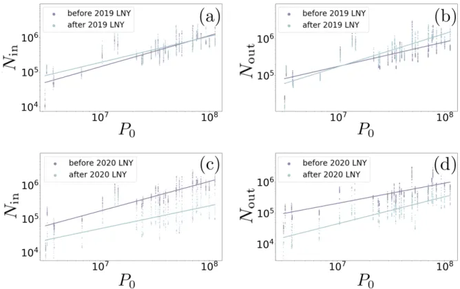
We observe a power law relationship between the incoming/outgoing flows and city population in Fig. S2 which indicates that the larger a city and the more flows it carries. Compared to 2019, the differences between the scatter points for incoming flows corresponding to days before and after LNY are much larger in 2020. This result emphasizes again that travel ban causes indeed the sharp drop of standard deviation in Fig. 1 (b) of the main text rather than the low travel intention during the Spring Festival.
The power law fits that we obtain imply that Nin∼ P γin
0 where γin≈ 0.93 before LNY and γin≈ 0.88 after LNY.
Similarly for outgoing flows we obtain γout ≈ 0.85 before and γout ≈ 0.93 after LNY. We can interpret these results
as a consequence of the conservation of the number of individuals traveling before and after LNY.
Distribution of Nin,out for 2020
We show the distribution, average and standard deviation of incoming/outgoing flows in Fig. S3. We observe that these distributions are relatively broad, in particular outgoing flows (Fig. S3 (a) and (b)). We show the standard deviation of incoming flows and outgoing flows over cities for each day, and the corresponding average (the same for the incoming and outgoing flows) in Fig. S3 (c). Note that the standard deviation of Nin is smaller than that of Nout
that people go to a relative large number of hometowns from a relative small number of workplaces before the Spring Festival; Due to the travel ban, people do not come back after the Spring Festival.
Distribution of Nin,out for 2019
We show the same quantities as above but for the year 2019. Here also, we observe broad distributions both for all incoming flows and all outgoing flows are shown in Fig. S4.
Fluctuations are larger around LNY where the total flow of individuals is larger, allowing for more heterogeneity. Before LNY individuals move from a large variety of cities to a relatively small number of hometowns explaining the large fluctuations of Nout. After LNY, individuals are returning from a small number of hometowns to a large variety
of cities, inducing large fluctuations of Nin. The corresponding dispersion and relative dispersions ∆outd ) and ∆ in d) are
shown in figures S4 (c) and (d). This also results in the heterogeneous distribution for the relative standard deviation of Nin and Nout averaged over cities for 2019 in Fig. S4 (e).
Gini indices for Nin,out
We compute Gini indices for cities. Instead of showing results for all cities, we plot Gini indices versus the traffic flows to or from cities in set {i ∈ V| min
d {maxd { Nin(i,d)
Nout(i,d)}, maxd {
Nout(i,d)
Nin(i,d)}} > 4.5} and Wuhan in Fig. S5. In this
case from these cities, many people go out to or come in from many different cities. These cities are critical and include Shanghai, Beijing, and so on. Due to travel bans, Wuhan exhibits specific features of scatter points with clear separation before and after LNY (see the scatter points in blue at the upper left corner corresponding to Wuhan in Fig. S5).
We also observe here in both cases a decreasing behavior on average. This is more salient for Nout where the trend
is clearly visible. This indicates that for larger outgoing flows, the Gini is smaller with no clearly dominant flow.
Statistical structure of the national population
We first show the population distribution in Fig. S6 (a). We observe a broad distribution and a power law fit gives the exponent α ≈ 5. We also show the number of important cities quantified by the integer part of n[1 − G(d)], in Fig. S6 (b).
Pendular ratio
In order to test the dependence of the pendular ratios on the criteria for defining classes, we change the criteria as follows: here if the value of R(i, 1) is larger than 1.2, we classify city i as a ‘receiver’ city. If the value is less than 0.8, we classify city i as an ‘emitter’ city. Finally, if the value is between 0.8 and 1.2, we classify city i as a ‘transit’ city. We show the location of three categories of cites on the map of China for 2019 and 2020 in Fig. S7.
Compared to the criteria in the main text, the number of transit cities decreases, while the number of emitter and receiver cities increases. However, as shown in Fig. S8, the patterns of the average value of pendular ratio corresponding to three categories of cites remain unchanged.
Statistics at the inter-province level Statistics of flows
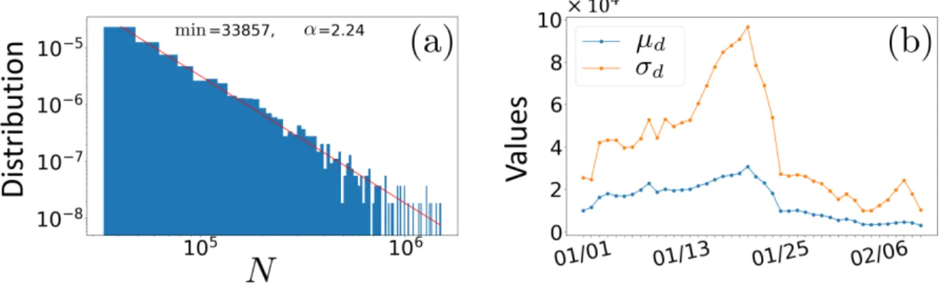
In what follows, we show some corresponding results based on province-level data instead of city-level data. The distribution of traffic flows between provinces exhibits large heterogeneity with the exponent of power law fit α around 2.24, as shown in Fig. S9 (a). A sharp drop of the standard deviation after Jan. 25th is observed in Fig. S9 (b).
We show the relative standard deviation of N over flows versus time with an order around 2.96 in Fig. S10 (a) and the distribution of the relative standard deviation of N over time concentrating around 0.64 in Fig. S10 (b). Large heterogeneity of traffic flows between provinces confirms the difficulty of modeling these flows. The relative standard
deviations corresponding to incoming and outgoing flows with smaller relative dispersions are shown in figures S10 (c) and (d).
We compare the incoming flows and outgoing flows versus city population in 2019 and 2020 at province-level with days before and after LNY highlighted by different colors in Fig. S11. Compared to 2019 (figures S11 (a) and (b)), the differences between days before and after LNY are much larger in 2020 (figures S11 (c) and (d)).
Statistical structure of the national population
The trends of the population Gini index for 2019 and 2020 are shown in Fig. S12. The Gini index reaches its maximum around LNY and returns to normal state gradually. Compared to 2019, the Gini index corresponding to 2020 has a higher peak and decreases with a slower speed.
We apply the criteria of three categories of provinces similar to that for city: If the value of R(i, 1) is larger than 1.2, we classify province i as a ‘receiver’ province. If the value is less than 0.8, we classify province i as an ‘emitter’ province. Finally, if the value is between 0.8 and 1.2, we classify province i as a ‘transit’ province. We show the location of three categories of cites on map of China for 2019 and 2020 in Fig. S13 and observe that receiver provinces are the majority in 2019 while emitter provinces are the majority in 2020. This results seem to make sense since most people defer the return time due to the travel ban, so that most provinces are ‘emitters’ in 2020.
We show in figures S14 (a) and (b) the pendular ratio for 2019 and 2020 for all provinces and highlight 5 provinces: Hubei, Beijing, Tianjin, Chongqing and Shanghai, corresponding to the origin province of COVID-19 and four province-level municipalities. We note that the curve corresponding to Hubei is in the bottom from all provinces in Fig. S14 (b), indicating that except Wuhan, the origin city of COVID-19, people also avoid going to cities of Hubei. We observe that, in 2019, the pendular ratios of all the three types of cities return to 1, meaning that the majority of individuals who went away for the holidays came back, as shown in Fig. S14 (c). The situation for 2020 is very different with a pendular ratio for all types of cities that converges to a value less than 1, indicating that the majority of people who went away for the holidays did not back yet, as shown in Fig. S14 (d).
To sum up, we show that the traffic flows between provinces are very heterogeneous, and display both large temporal and spatial fluctuations, and so on. These results for province-level are in good agreement with for city-level, indicating that our methods are applicable to both scales. Despite the detailed characters of traffic flows revealed by results for city-level and province-level, a global view of a higher level is also necessary. The statistical properties of the interurban mobility help us to understand the effect of travel restrictions, their impact on and the control of epidemic spread.
Figure S1: Average and standard deviation of N over traffic flows versus time for 2019 with the corresponding migration ratio for 2020.
Figure S2: Incoming flows (a) and outgoing flows (b) for all cities and days versus city population before and after the 2019 LNY in loglog. Incoming flows (c) and outgoing flows (d) for all cities and days versus city population before and after the 2020 LNY in loglog.
Figure S3: Observation of incoming and outgoing flows for 2020. (a) Distribution of all incoming flows in loglog with parameters of power law fitting on the top middle. (b) Distribution of all outgoing flows in loglog with parameters of power law fitting on
Figure S4: Observation of incoming and outgoing flows for 2019. (a) Distribution of all incoming flows in loglog with parameters of power law fitting on the top middle. (b) Distribution of all outgoing flows in loglog with parameters of power law fitting on
the top middle. (c) Average and standard deviation of Ninand Noutover cities versus time. (d) Relative standard deviation of
Nin and Noutover cities versus time. (e) Distribution of the relative standard deviation of Nin and Noutover time.
Figure S6: (a) Distribution of populations of all cities in loglog. (b) The number of important cities versus time corresponding to 2019 and 2020. We match the time scale for 2019 and 2020 according to LNY (for the sake of clarity, we show on the x-axis the dates for 2020 only). The vertical line highlights the LNY.
Figure S7: (a) Emitter, receiver and transit cities according to the value of R(i, 1) for 2019 with the number of three categories of provinces at the lower left corner. (b) Emitter, receiver and transit cities according to the value of R(i, 1) for 2020 with the number of three categories of provinces at the lower left corner.
Figure S8: (a) Mean value of the pendular ratios over cities according to the classification (receiver, emitter or transit cities) with different criteria versus days from LNY in 2019. The colored areas correspond to one standard deviation. (b) Mean value of the pendular ratios over cities according to the classification with different criteria versus days from LNY in 2020 with shaded areas representing standard deviation.
Figure S9: (a) Distribution of all traffic flows N (i, j, d) in loglog. The line is a power law fit of the form N−αwith exponent α = 2.27. (b) Average and standard deviation of N over traffic flows versus time.
Figure S10: (a) Relative standard deviation of N over traffic flows versus time. (b) Distribution of the relative standard
deviation of N over time. (c) Relative standard deviation of Ninand Nout over provinces versus time. (d) Distribution of the
Figure S11: Incoming flows (a) and outgoing flows (b) for all provinces and days versus province population before and after the 2019 LNY in loglog. Incoming flows (c) and outgoing flows (d) for all provinces and days versus province population before and after the 2020 LNY in loglog.
Figure S12: Temporal variations during the Spring Festical of the population Gini index for 2019 and 2020. The dotted line represents the value ‘at rest’.
Figure S13: (a) Emitter, receiver and transit provinces according to the value of R(i, 1) for 2019 with the number of three categories of provinces at lower left corner. (b) Emitter, receiver and transit provinces according to the value of R(i, 1) for 2020 with the number of three categories of provinces at lower left corner.
Figure S14: Comparison of pendular ratio between 2019 and 2020. (a) Pendular ratio for all provinces versus days df from LNY
in 2019. We highlighted five important provinces. (b) Pendular ratio for all provinces versus days df from LNY in 2020 with
highlight of 5 provinces. (c) Mean values of the pendular ratio over provinces according to the classification (receiver, emitter or transit provinces) versus days from LNY in 2019. The colored areas correspond to one standard deviation. (d) Mean value of the pendular ratio over provinces according to the classification versus days from LNY in 2020 with colorbar representing standard deviation.